Computing the Depth of a Flat

Abstract

We compute the regression depth of a $k$-flat in a set of $n$ points $\Bbb R^{d}$, in time $O(n^{d-2}+n\mathop{{\rm log}}n)$ when $1\leq k\leq d-2$. In constrast, the best time bound known for the $k=0$ case (data depth) or for the $k=d-1$ case (hyperplane regression) is $O(n^{d-1}+n\mathop{{\rm log}}n)$.

1 Introduction

Regression depth was introduced by Hubert and Rousseeuw [9] as a distance-free quality measure for linear regression. The depth of a hyperplane with respect to a set of data points in $\Bbb R^{d}$ is the minimum number of data points crossed in any continuous motion taking the hyperplane to a vertical hyperplane. A vertical hyperplane is a regression failure, because it allows the response variable (that is, the dependent variable) to vary over its entire range while keeping the explanatory variables (the independent variables) fixed. Thus a good regression plane should be far from a vertical hyperplane. A deepest hyperplane is farthest from vertical in a combinatorial sense; it provides a good fit even in the presence of skewed or data-dependent errors, and is robust against a constant fraction of arbitrary outliers.

Due to its combinatorial nature, the notion of regression depth leads to many interesting algorithmic and geometric problems. For points on the line $R^{1}$, a median point is a point of maximum depth. For the case of $n$ points in the plane $R^{2}$, Hubert and Rousseeuw [4] gave a simple construction called the catline, which finds a line of depth $\lceil n/3\rceil$. The deepest line in the plane can be found in time $O(n\mathop{{\rm log}}n)$ [5]. The catline’s depth bound is best possible, and more generally in $\Bbb R^{d}$ the best depth bound is $\lceil n/(d+1)\rceil$ [1, 6]. The fastest known exact algorithm for maximizing depth takes time $O(n^{d})$, and $\epsilon$-cutting techniques can be used to obtain an $O(n)$-time $(1+\epsilon)$-approximation to the maximum depth [11].

In previous work [2], we generalized depth to multivariate regression, that is, fitting points in $\Bbb R^{d}$ by affine subspaces with dimension $k<d-1$ ($k$-flats for short). We showed that for any $d$ and $k$, deep $k$-flats always exist, meaning that for any point set in $R^{d}$, there is always a $k$-flat of depth a constant fraction of $n$, with the constant depending on $d$ and $k$. This result implies that the deepest flat is robust, with a breakdown point which is a constant fraction of $n$. We also generalized the catline construction to find lines with depth $\lceil n/(2d-1)\rceil$, which is tight for $d\leq 3$ and would be tight for all $d$ under a conjectured $\lceil n/((k+1)(d-k)+1)\rceil$ bound on maximum regression depth. On the algorithmic side, we showed that $\epsilon$-cuttings can be used to obtain an $O(n)$-time $(1+\epsilon)$-approximation for the deepest flat.

In this paper, we consider the problem of testing the depth of a given flat, or more generally the crossing distance between two flats. Rousseeuw and Struyf [10] studied similar problems for hyperplanes and points. The crossing distance between a point and a hyperplane can be found in time $O(n^{d-1}+n\mathop{{\rm log}}n)$ by examining the arrangement’s restriction to the hyperplane (as described later), and the same bound applies to testing the depth of a hyperplane or point. We show that, in contrast, the depth of a flat of any other dimension can be found in randomized time $O(n^{d-2}+n\mathop{{\rm log}}n)$. More generally, the crossing distance between a $j$-flat and a $k$-flat can be found in time $O(n^{\,j+k-1}+n\mathop{{\rm log}}n)$ when $1\leq j,k\leq d-2$.

2 Definitions

A generic $k$-flat with $k<d-1$ can move continuously to vertical without crossing any data points, so it is not obvious how to generalize regression depth to $k$-flats. The key is to start from an equivalent definition of hyperplane regression depth: the depth of a hyperplane ${\cal H}$ is the minimum number of data points in a double wedge with one boundary equal to ${\cal H}$ and the other boundary vertical (parallel to the response variable’s axis). A double wedge is the closed region bounded by two hyperplanes; it is the region necessarily swept out by a continuous motion of one bounding hyperplane to the other.

Now consider the simplest example with $k<d-1$, the regression depth of a line in $\Bbb R^{3}$. We think of $x$ as the explanatory variable, and $y$ and $z$ as two response variables. A regression line simultaneously explains $y$ and $z$ as linear functions of $x$, and any line parallel to the $yz$-plane is a regression failure that allows $y$ and $z$ to vary over their entire range while keeping $x$ fixed. We would thus like our regression line to be far from lines parallel to the $yz$-plane. A reasonable guess at the definition of regression depth of a line ${\cal L}$ would be the minimum number of data points in a double wedge with one boundary containing ${\cal L}$ and the other boundary parallel to the $yz$-plane.

This guess indeed turns out to be the correct generalization; its naturalness is revealed by looking at the dual formulation of the problem. The projective dual of a point set is a hyperplane arrangement, and hyperplane regression dualizes to finding a central point in an arrangement. If the depth of a point $p$ is the minimum number of arrangement hyperplanes crossed by any line segment from $p$ to the hyperplane at infinity, then (as observed by Rousseeuw) the regression depth of a hyperplane is exactly the depth of its dual point in the dual arrangement. We generalized this observation to give a natural distance measure between flats in an arrangement [2].

Definition 1

The crossing distance between two flats in an arrangement is the fewest hyperplane crossings along any line segment having one endpoint on each flat.

In the primal formulation, the crossing distance is the minimum number of points in a double wedge with one boundary containing one flat and the other boundary containing the other.

Definition 2

The regression depth of a $k$-flat is the crossing distance between its dual $(d-k-1)$-flat and a $k$-flat at vertical infinity.

For multivariate regression, the $k$-flat at vertical infinity should be the one dual to the intersection of the hyperplane at infinity with the $(k-d)$-flat spanned by the response variable axes. With this choice, regression failures have regression depth zero. For hyperplane regression, there is no choice to make as there is only one $(d-1)$-flat at infinity.

Along with hyperplane regression, Definition 2 also subsumes the classical notion of data depth or Tukey depth. The data depth of a point $p$ is the minimum number of data points in any closed half-space—a degenerate double wedge—containing $p$. The data depth of $p$ is also the crossing distance of its dual hyperplane from the point at vertical infinity.

3 Reduction to Covering

We now show that crossing distance can be reduced to finding a minimally covered point in a certain family of sets. Suppose we are given an arrangement of hyperplanes, a $j$-flat ${\cal F}_{1}$, and a $k$-flat ${\cal F}_{2}$. We wish to determine the line segment, having one endpoint on each flat, that crosses as few arrangement hyperplanes as possible.

We first parametrize the space of relevant line segments. Without loss of generality the two flats do not meet (else the crossing distance is zero) so any pair of points from ${\cal F}_{1}\times{\cal F}_{2}$ determines a unique line. The pair divides the line into two complementary line segments (one through infinity), so we need to augment each point of ${\cal F}_{1}\times{\cal F}_{2}$ by an additional bit of information to specify each possible line segment. We do this topologically: ${\cal F}_{1}$ is a projective space, having as its double cover a $j$-sphere ${\cal S}_{1}$, and similarly the double cover of ${\cal F}_{2}$ is a $k$-sphere ${\cal S}_{2}$. The product ${\cal S}_{1}\times{\cal S}_{2}$ supplies two extra bits of information per point, and there is a continuous two-to-one map from ${\cal S}_{1}\times{\cal S}_{2}$ to the line segments connecting the two flats.

Now consider subdividing ${\cal S}_{1}\times{\cal S}_{2}$ according to whether the corresponding line segments cross or do not cross a hyperplane ${\cal H}$ of the arrangement. The boundary between crossing and non-crossing line segments is formed by the segments with an endpoint on a great sphere formed by intersecting ${\cal H}$ with ${\cal S}_{1}$ or ${\cal S}_{2}$. The line segments that cross ${\cal H}$ therefore correspond to a set $({\cal H}_{1}\times\overline{\cal H}_{2})\cup(\overline{\cal H}_{1}\times{\cal H}_{2})$, where ${\cal H}_{i}$ is a hemisphere bounded by the intersection of ${\cal H}$ with ${\cal S}_{i}$. A line segment crossing the fewest hyperplanes then corresponds to a point in the fewest such sets.

For example, Figure 1 illustrates the case in which ${\cal F}_{1}$ and ${\cal F}_{2}$ are each lines. The space of line segments with one endpoint on ${\cal F}_{1}$ and the other endpoint on ${\cal F}_{2}$ is doubly covered by the two-dimensional torus ${\cal S}_{1}\times{\cal S}_{2}$, which we have cut along two circles to show as a square. The solid dots represent the same line segment; the hollow dots represent the complementary line segment. Three covering sets of the form $({\cal H}_{1}\times\overline{\cal H}_{2})\cup(\overline{\cal H}_{1}\times{\cal H}_{2})$ are shown; their boundaries are shown dotted, dashed, and solid respectively, and the interiors of the sets are shaded. (The dotted boundary happens to align with the circles that cut the torus down to a square.)

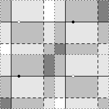
Figure 1: Computing the crossing distance between two lines (1-flats) is equivalent to finding a minimally covered point on the torus ${\cal S}_{1}\times{\cal S}_{2}$.

Since the union in each set of the form $({\cal H}_{1}\times\overline{\cal H}_{2})\cup(\overline{\cal H}_{1}\times{\cal H}_{2})$ is a disjoint union, we can simplify the problem a bit by cutting each such set into two products of hemispheres. We summarize the discussion above with a lemma.

Lemma 1

Computing the crossing distance between flats ${\cal F}_{1}$ and ${\cal F}_{2}$ is equivalent to finding a point in a product of spheres ${\cal S}_{1}\times{\cal S}_{2}$ that is covered by the fewest sets from a given family of subsets, each of which is a product of hemispheres ${\cal H}_{1}\times{\cal H}_{2}$.

4 Algorithms

We now show how to solve the problem given in Lemma 1. We first consider the special case of the crossing distance between a point and hyperplane, that is, $j=0$ and $k=d-1$. In this case, the product of spheres is a disjoint pair of $(d-1)$-spheres, both covered identically by a family of hemispheres, so we can treat it as if it were just a single sphere. We would like to find a point on this sphere that is covered by the fewest hemispheres. We can build the entire arrangement of hemispheres in time $O(n^{d-1}+n\mathop{{\rm log}}n)$ using a slight modification of an algorithm for computing a hyperplane arrangement [3], and compute the number of hemispheres covering each cell by stepping from cell to cell in constant time per step. Any minimally covered cell gives a solution.

Next let us consider the special case of the crossing distance between two lines, that is, $j=k=1$. The product of spheres ${\cal S}_{1}\times{\cal S}_{2}$ is just a 2-torus, and the products of hemispheres are just products of semicircles. We cut the torus into a square as in Figure 1; each product of semicircles turns into a set of at most four rectangles. We refer to the horizontal and vertical projections of these rectangles as segments.

We can now use a standard sweep-line algorithm to compute a point in ${\cal S}_{1}\times{\cal S}_{2}$ covered by a minimum number of sets. Conceptually we sweep a vertical line from left to right across Figure 1. We use a segment tree [8] to represent the vertical segments crossed by the sweep line; let us assume that vertical represents ${\cal S}_{2}$. As usual with segment trees, each vertical segment ${\cal H}_{2}$ appears at $O(\mathop{{\rm log}}n)$ nodes of the segment tree, exactly those nodes whose intervals are covered by ${\cal H}_{2}$ but whose parents’ intervals are not covered by ${\cal H}_{2}$. (Here we denote vertical segments by ${\cal H}_{2}$, even though some of them are just “halves” of the original semicircles ${\cal H}_{2}$.)

We equip each node $v$ of the segment tree with an additional piece of information: the minimum number of ${\cal H}_{2}$ segments covering some point in the interval corrresponding to $v$. This coverage number can be computed by taking the minimum of the numbers at $v$’s two children and adding the number of segments listed at $v$ itself.

We sweep horizontally across the square. The events in the sweep algorithm correspond to endpoints of segments on ${\cal S}_{1}$. At each endpoint of a segment we update the segment tree along with the coverage numbers at its nodes. Coverage numbers change at only $O(\mathop{{\rm log}}n)$ nodes: the ancestors of the nodes storing the newly inserted or deleted vertical segment. The coverage number at the root gives the minimally covered cell currently crossed by the sweep line. We also maintain the overall minimum covering seen so far, and update this minimum at each event. At the end of the sweep, the overall minimum gives the answer. We have obtained the following theorem.

Theorem 1

The crossing distance between two lines in an arrangement in $\Bbb R^{d}$, or the regression depth of a line in $\Bbb R^{3}$, can be found in time $O(n\mathop{{\rm log}}n)$.

For general $j$ and $k$, we use a randomized recursive decomposition in place of the segment tree.

Lemma 2

Given an arrangement of hyperplanes in $\Bbb R^{d}$, we can produce a recursive binary decomposition of $\Bbb R^{d}$, with high probability in time $O(n^{d}+n\mathop{{\rm log}}{n})$, such that any halfspace bounded by an arrangement hyperplane has (with high probability) a representation as a disjoint union of decomposition cells with $O(n^{d-1}+\mathop{{\rm log}}{n})$ ancestors.

Proof sketch: We apply a randomized incremental arrangement construction algorithm. Each cell in the recursive decomposition is an arrangement cell at some stage of the construction. The bound on the representation of a halfspace comes from applying the methods of [7, pp. 120–123] to the zone of the boundary hyperplane.   

The same method applies essentially without change to spheres and hemispheres, so we can apply it to the sets occurring in Lemma 1. Each product of hemispheres occurring in Lemma 1 can be represented as disjoint unions of $O(n^{\,j+k-2})$ products of cells in the product of the two recursive decompositions formed by applying Lemma 2 to ${\cal S}_{1}$ and ${\cal S}_{2}$. Since there are $O(n)$ products of hemispheres, we have overall $O(n^{\,j+k-1})$ products of cells.

The algorithm has a similar structure to the algorithm for the case $j=k=1$, only the simple sweep order for processing the cells of ${\cal S}_{1}$ is replaced by a depth-first traversal of the recursive decomposition of ${\cal S}_{1}$. As in the sweep algorithm, we maintain a coverage number for each cell of the decomposition of ${\cal S}_{2}$. The coverage number measures the fewest ${\cal H}_{2}$ hemispheres covering some point in that cell, where the ${\cal H}_{2}$ hemispheres come from pairs ${\cal H}_{1}\times{\cal H}_{2}$ for which ${\cal H}_{1}$ covers the current cell in the traversal of ${\cal S}_{1}$. These numbers are computed by taking the minimum number for the cell’s two children and adding the number of hemispheres whose decomposition uses that cell directly. When the traversal visits a cell in ${\cal S}_{1}$, we determine the set of hemispheres whose decomposition uses that cell, and update the numbers for the ancestors of cells covering the corresponding hemispheres in ${\cal S}_{2}$. Each hemisphere product leads to $O(n^{\,j+k-2})$ update steps, so the total time for this traversal is $O(n^{\,j+k-1})$. We also maintain the overall minimum covering seen so far, and take the minimum with the number at the root of the decomposition of ${\cal S}_{2}$ whenever the depth-first traversal reaches a leaf in the decomposition of ${\cal S}_{1}$.

When one flat—say ${\cal F}_{1}$—is a line, this method’s time includes an unwanted logarithmic factor. To avoid this factor, we return to a sweep algorithm as the case $j=k=1$. We sweep across ${\cal S}_{1}$, using the hierarchical decomposition data structure for ${\cal S}_{2}$ in place of the segment tree. When the traversal reaches an endpoint of an interval ${\cal H}_{1}$, we update the cells for the corresponding hemisphere ${\cal H}_{2}$.

We summarize with the following theorem. It is likely that $\epsilon$-cuttings can derandomize this result.

Theorem 2

The crossing distance between a $j$-flat and a $k$-flat can be found with high probability in time $O(n^{\,j+k-1}+n\mathop{{\rm log}}n)$ for $1\leq j,k$. The depth of a $k$-flat for $1\leq k\leq d-2$ can be found in time $O(n^{d-2}+n\mathop{{\rm log}}n)$ with high probability.

References

- [1] N. Amenta, M. Bern, D. Eppstein, and S.-H. Teng. Regression depth and center points. Discrete & Computational Geometry 23(3):305–323, 2000, cs.CG/9809037.
- [2] M. Bern and D. Eppstein. Multivariate regression depth. Proc. 16th Symp. Computational Geometry, pp. 315–321. ACM, June 2000, cs.CG/9912013.
- [3] H. Edelsbrunner. Algorithms in Combinatorial Geometry. EATCS Monographs on Theoretical Computer Science 10. Springer Verlag, 1987.
- [4] M. Hubert and P. J. Rousseeuw. The catline for deep regression. J. Multivariate Analysis 66:270–296, 1998, http://win-www.uia.ac.be/u/statis/publicat/catline_abstr.html.
- [5] S. Langerman and W. Steiger. An algorithm for the hyperplane median in . Proc. 11th Symp. Discrete Algorithms, pp. 54–59. ACM and SIAM, January 2000.
- [6] I. Mizera. On depth and deep points: a calculus. Inst. Mathematical Statistics Bull. 27(4), 1998, http://www.dcs.fmph.uniba.sk/~mizera/PS/depthps.ps. Full version to appear in Annals of Statistics.
- [7] K. Mulmuley. Computational Geometry: An Introduction Through Randomized Algorithms. Prentice-Hall, 1994.
- [8] F. P. Preparata and M. I. Shamos. Computational Geometry: An Introduction. Springer Verlag, 1985.
- [9] P. J. Rousseeuw and M. Hubert. Regression depth. J. Amer. Statistical Assoc. 94(446):388–402, June 1999, http://win-www.uia.ac.be/u/statis/publicat/rdepth_abstr.html.
- [10] P. J. Rousseeuw and A. Struyf. Computing location depth and regression depth in higher dimensions. Statistics and Computing 8(3):193–203, August 1998, http://win-www.uia.ac.be/u/statis/publicat/compdepth_abstr.html.
- [11] W. Steiger and R. Wenger. Hyperplane depth and nested simplices. Proc. 10th Canad. Conf. Computational Geometry. McGill Univ., 1998, http://cgm.cs.mcgill.ca/cccg98/proceedings/cccg98-steiger-hyperplane.ps%.gz.