Pattern Matching for Sets of Segments

In this paper we present algorithms for a number of problems in geometric pattern matching where the input consist of a collections of segments in the plane. Our work consists of two main parts. In the first, we address problems and measures that relate to collections of orthogonal line segments in the plane. Such collections arise naturally from problems in mapping buildings and robot exploration.

We propose a new measure of segment similarity called a coverage measure, and present efficient algorithms for maximising this measure between sets of axis-parallel segments under translations. Our algorithms run in time $O(n^{3}\mbox{\sl polylog}\,n)$ in the general case, and run in time $O(n^{2}\mbox{\sl polylog}\,n)$ for the case when all segments are horizontal. In addition, we show that when restricted to translations that are only vertical, the Hausdorff distance between two sets of horizontal segments can be computed in time roughly $O(n^{3/2}\mbox{\sl polylog\,}n)$. These algorithms form significant improvements over the general algorithm of Chew et al.  that takes time $O(n^{4}\log^{2}n)$.

In the second part of this paper we address the problem of matching polygonal chains. We study the well known Fréchet distance , and present the first algorithm for computing the Fréchet distance   under general translations. Our methods also yield algorithms for computing a generalization of the Fréchet distance, and we also present a simple approximation algorithm for the Fréchet distance  that runs in time $O(n^{2}\mbox{\sl polylog}\,n)$.

1 Introduction

Traditionally, geometric pattern matching employs as a measure of similarity the Hausdorff distance h(A,B), defined as $h(A,B)=\max_{p\in A}~{}\min_{q\in B}~{}d(p,q)$ for two point sets $A$ and $B$. However, when the patterns to be matched are line segments or curves (instead of points), this measure is less than satisfactory. It has been observed that measures like the Hausdorff measure that are defined on point sets are ill-suited as measures of curve similarity, because they destroy the continuity inherent in continuous curves.

This paper addresses problems in geometric pattern matching where the inputs are sets of line segments. Our work consists of two main parts; in the first part we consider the problem of matching (under translation) segments that are axis-parallel (i.e either horizontal or vertical), and in the second we consider the problem of matching polygonal chains under translation. We study two different measures in this context; the first is a novel measure called the coverage measure, which captures the similarity between orthogonal segments that may partially overlap with one another. The other is the well known Fréchet distance, first proposed by Maurice Fréchet in 1906 as a measure of distance between distributions, which has often been referred to as a natural measure of curve similarity [4, 17, 27]. We discuss each measure in detail below.

1.1 Mapping and orthogonality

The motivation for considering instances of pattern matching where the input line segments are orthogonal comes from the domain of mapping, in which a robot is required to map the underlying structure of a building by moving inside the building, and “sensing” or “studying” its environment.

In one such mapping project at the Stanford Robotics laboratory the robot is equipped with a laser range finder which supplies the distance from the robot to its nearest neighbor in a dense set of directions in a horizontal plane. We call the resulting distances map a picture. Figure 1(a) shows the robot used at Stanford for this purpose the laser range finder installed on the robot.

During the mapping process, the robot must merge into a single map the series of pictures that it captures from different locations in the building.

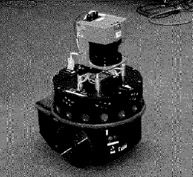
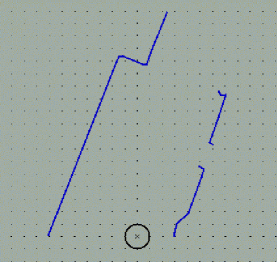
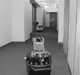
Figure 1: Left: The robot, and the laser range finder installed on it. Middle: Typical “picture” obtained by the robot of a corridor (after segmentation). Right: The corridor itself

Since the dead reckoning of the robot is not very accurate, it cannot rely solely on its motion to decide how the pictures are placed together. Thus, we need a matching process that can align (by using overlapping regions) the different pictures taken from different points of the same environment. In addition, we need to determine whether the robot has returned to a point already visited. We make the reasonable assumption that buildings walls are almost always either orthogonal or parallel to each other, and that these walls are frequently by far the most dominant objects in the pictured. This is especially significant in the case that the robot is inside a corridor, where there is a lack of detail needed for good registration. In some cases most of the picture consists merely of two walls with a small number of other segments. See Figure 1(b),(c) for a typical picture and the real region that the laser range finder senses.

This application suggests the study of matching sets of horizontal and vertical segments. Observe that we may restrict ourself to alignments under translation, as it is easy to find the correct rotation for matching sets of orthogonal segments. Formally, let $A=\{a_{1}\dots a_{n}\}$ and $B=\{b_{1},\dots b_{n}\}$ be two sets of orthogonal line segments in the plane, and let $\varepsilon$ be a given parameter. A point $p$ of a horizontal (resp. vertical ) segment $a\in A$ is covered if there is a point of a horizontal (resp. vertical) segment $b\in B$ whose distance from $p$ is $\leq\varepsilon$, where the distance is measured using the $\ell_{\infty}$ norm. Let $w(A,B)$ denote the collection of sub-segments of $A$ consisting of covered points. Let $\mbox{\sl Cov}(A,B)$ be the total length of the segments of $w(A,B)$. The maximum coverage problem is to find a translation $t^{*}$ in the translation plane (TP ) that maximizes $\mbox{\sl Cov}(t)=\mbox{\sl Cov}(t+A,B)$. To the best of our knowledge, this measure is novel.

The coverage measure is especially relevant in the case of long segments e.g. inside a corridor, when we might be interested in partially matching portions of long segments to portions of other segments.

Our Results

In Section 2 we present an algorithm that solves the Coverage problem between sets of axis-parallel segments in time $O(n^{3}\log^{2}n)$ and the Coverage problem between horizontal segments in time $O(n^{2}\log n)$ Note that the known algorithms for matching arbitrary sets of line segments are much slower. For example, the best known algorithm for finding a translation that minimizes the Hausdorff Distance between two sets of $n$ segments in the plane runs in time $O(n^{4}\log^{2}n)$ [3, 10]. We also show that the that the combinatorial complexity of the Hausdorff matching between segments is $\Omega(n^{4})$, even if all segments are horizontal. This strengthens the bounds shown by Rucklidge [15], and demonstrates that our algorithms, much like the algorithms of [8, 9] are able to avoid having to examine each cell of ${\cal F}$ individually. Note that all our results extend to the case when segments are weighted and the coverage is now a weighted sum of interval lengths.

In Section Section 3 we consider the related problem of matching horizontal segments under vertical translations (under the Hausdorff measure). It has been observed that if horizontal translations are allowed, then this problem is 3SUM-hard [6], indicating that finding a sub-quadratic algorithm may be hard. However, we present an algorithm running in time $O(n^{3/2}\max\{\log^{c}M,\log^{c}n,1/\varepsilon^{c}))\}$, for some fixed constant $c$, which is sub-quadratic in most cases. Here, $M$ denotes the ratio of the diameter to the closest pair of points in the sets of segments (where pairs of points must lie on different segments).

1.2 The Fréchet distance 

In the second part of the paper, we consider measures for matching polygonal chains under the Fréchet distance. Let us define a curve as a continuous mapping $P:[a,a^{\prime}]\rightarrow{\Bbb R}^{2}$. The Fréchet distance between two curves $P$ and $Q$, $d_{F}(P,Q)$ is defined as:

$$d_{F}(P,Q)=\inf_{\alpha,\beta}\max_{t\in[0,1]}\|f(\alpha(t))-g(\alpha(t))\|$$

where $\alpha,\beta$ range over continuous increasing functions from $[0,1]\rightarrow[a,a^{\prime}]$ and $[0,1]\rightarrow[b,b^{\prime}]$ respectively.

Alt and Godau proposed the first algorithm for computing the Fréchet distance  between two polygonal chains (with no transformations). Their method is elegant and simple, and runs in time $O(pq)$, where $p$ and $q$ are the number of segments in the two polygonal chains. In his Ph.D thesis [21]. Michael Godau presents an extensive study of the complexity of computing the Fréchet distance. He shows that computing the Fréchet distance  between two simplicial objects is NP-hard, for any dimension $d\geq 3$.

Although the Fréchet distance is a natural measure for curve similarity, its applicability has been limited by the fact that no algorithms exist to minimise the Fréchet distance between curves under various transformation groups. Prior to our work, the only result on computing the Fréchet distance  under transformations was presented by Venkatasubramanian [26]. He computes $\min_{t\in TP_{x}}d_{F}(P,Q+t)\leq\varepsilon$, where $TP_{x}$ is the set of translations along a fixed direction, in time $O(n^{5}\mbox{\sl polylog\,}n)$ (where $n=p+q$). In fact, our methods can be viewed as a generalization of his methods and can be used to solve his problem in the same time bound.

Our Results

In Section 4 we present the first algorithm for computing the Fréchet distance  between two polygonal chains minimized under translations. The algorithm is based on a reduction to a dynamic graph reachability problem; its running time is $O(n^{10}\mbox{\sl polylog}\,n)$.

If we drop the restriction that the functions $\alpha,\beta$ must be increasing, we obtain a measure that we call the weak Fréchet distance , denoted by $d_{\tilde{F}}$. Our methods can be used to decide whether $\min_{t\in TP}d_{\tilde{F}}(P,Q+t)\leq\varepsilon$; in this case, the underlying graph is undirected, yielding an algorithm that runs in time $O(n^{4}\mbox{\sl polylog}\,n)$.

With the exact algorithms being rather expensive, it is natural to ask whether approximations can be obtained efficiently. A simple observation shows that we can obtain an $(\varepsilon,\beta)$-approximation to the Fréchet distance  under translations in time $O(n^{2}{{\sl poly}}(\log n,1/\beta))$.

2 Maximum Coverage Among Sets Of Segments

Let $A=\{a_{1}\dots a_{n}\}$ and $B=\{b_{1},\dots b_{n}\}$ be two sets of axis-parallel line segments in the plane, and let $\varepsilon$ be a given parameter. Recall the coverage measure $\mbox{\sl Cov}(A,B)$ as defined in the introduction.

2.1 Computing coverage with axis-parallel segments

We first consider the case that the sets $A$ and $B$ consists of both horizontal and vertical segments. Let $A^{h}$ (resp. $B^{h}$) be a set of $n$ horizontal segments and let $A^{v}$ (resp. $B^{v}$) be a set of $n$ vertical segments. Let $\varepsilon$ be a given parameter. Let $A=A^{h}\cup A^{v}$ and let $B=B^{h}\cup B^{v}$. Let $\mbox{\sl Cov}(t+A,B)=\mbox{\sl Cov}(t+A^{h},B^{h})+\mbox{\sl Cov}(t+A^{v},B^{v})$.

We first need the following lemma, whose proof is deferred to Appendix A. Let ${\cal S}=\{s_{1}\dots s_{m}\}$ be a set of non-vertical segments in ${\Bbb R}^{2}$. For each segment $s_{i}\in{\cal S}$ we define the functions $s_{i}(x)\rightarrow{\Bbb R}$ as follows: For every $x\in{\Bbb R}$, $s_{i}(x)$ is the $y$-coordinate of the intersection point of $s$ and the vertical line passing through $x$, if such an intersection point exists. We set $s_{i}(x)$ to be $0$ otherwise. Let $\mbox{\sl sum}_{\cal S}(x)=\Sigma_{i=1}^{m}s_{i}(x)$, and let $\max(\mbox{\sl sum}_{\cal S}(\cdot))=\max_{x\in{\Bbb R}}\mbox{\sl sum}_{\cal S}(x)$. Furthermore, let $T=T(\tau)$ be a subset of ${\cal S}$ consisting of horizontal segments that can move vertically at constant speed i.e the $y$-coordinates of the endpoints of each $s_{i}\in T$ are given by $y=a_{i}\tau+b_{i}$.

Lemma 2.1

Given a set of non-vertical segments $S$ with a subset $T$ of horizontal moving segments, we can maintain $\max(\mbox{\sl sum}_{\cal S}(\cdot))$ under segment insertions or deletions in amortized time $O(\sqrt{|}{\cal S}|)$ per operation. In addition, we can maintain $\max(\mbox{\sl sum}_{\cal S}(\cdot))$ under a time-decreasing step ($\tau\leftarrow\tau-\Delta$) in $O(1)$ time.

Theorem 2.2

We can find a translation $t$ that maximizes $\mbox{\sl Cov}(t+A,B)$ in time $O(n^{3}\log^{2}n)$, where $n=|A|+|B|$

Proof: The proposed algorithm is a line-sweep algorithm, with the sweep line moving from top to bottom. For a segment $b_{i}\in B$ let $b_{i}^{+}$ denote the rectangle consisting of all points whose $\ell_{i}nfty$ distance from $b_{i}$ is at most $\varepsilon$. Let $B^{+}$ denote the union $\bigcup_{i=1}^{n}b_{i}^{+}$. Note that any two rectangles $b_{i}^{+},b_{j}^{+}$ intersect in at most two points, so by [13] the complexity of the boundary of $B^{+}$ is $O(n)$. Consider $E=\{p_{1}\dots p_{2n}\}$, the set of the $2n$ endpoints of the segments of $A$. Define the layer $L_{i}=B^{+}-p_{i}$, which is the region in the TP  of all translations $t$ that shift $p_{i}$ into $B^{+}$ i.e $t+p_{i}\in B^{+}$. Let ${\cal B}^{h}$ (resp. ${\cal B}^{v}$) be the collection of layers created by the horizontal (resp. vertical) segments of $A$. As the line sweep traverses the translation plane from top to bottom, we encounter events where $\ell$ intersects a horizontal boundary segment of either ${\cal B}^{h}$ or ${\cal B}^{v}$.

Horizontal Boundaries Of ${\cal B}^{h}$: Let $\mbox{\sl Cov}(x):{\Bbb R}\rightarrow{\Bbb R}$ be the value of $\mbox{\sl Cov}(t+A^{h},B^{h})$, where $t$ is the point on $\ell$ vertically above $x$. Consider the contribution to $\mbox{\sl Cov}(t+A^{h},B^{h})$ from the interaction between the segments $a\in A^{h},b\in B^{h}$. This contribution to the function consists of a piecewise linear function, consists of five segments: It is zero for value of $x$ which are very far from the regions of interaction between $a$ and $b$, it is a constant that equals the minimum of the length of $a$ and $b$ when $x$ is near the region of intersection, and it consists of two segments of slopes are $1$ and $-1$, connecting these segments. These segments exist for all instances of the line sweep where its horizontal distance to the boundary of the rectangle of $B_{j}$ corrsponds to $a_{i}$ is $\leq\varepsilon$. There are $O(n^{2})$ update operations, and each update can be processed in $O(n\log^{2}n)$ time from Lemma Lemma 2.1.

Horizontal Boundaries Of ${\cal B}^{v}$. For two vertical segments $a_{i}\in A,b_{j}\in B$, let ${\cal T}_{ij}$ be the set of translations for which the horizontal distance from $a_{i}$ to $b_{j}$ is at most $\varepsilon$. Assume w.l.o.g that $|a_{i}|>|b_{j}|$. Let $UP_{ij}$ denote all translations $t$ for which the upper endpoint of $a_{i}$ is covered by $t+b_{j}$, (i.e. its distance from some point of $t+b_{j}$ is at most $\varepsilon$) but the lower endpoint of $a_{i}$ is not covered. Similarly, let $DOWN_{ij}$ denote all translations $t$ for which the lower endpoint of $a_{i}$ is covered by $t+b_{j}$, but the upper endpoint of $a_{i}$ is not covered and let $MID_{ij}$ denote all translations $t$ for which both endpoints of $a_{i}$ are covered.

Thus $\mbox{\sl Cov}(t+a_{i},b_{j})$ is zero when $t\notin UP_{ij}\cup MID_{ij}\cup DOWN_{ij}$, $\mbox{\sl Cov}(t+a_{i},b_{j})$ is a constant when $t\in MID_{ij}$, and it is a decreasing (resp. increasing) linear function that depends only on the $y$-coordinate of $t$ when $t\in UP_{ij}$ (resp.  $t\in DOWN_{ij}$). Therefore, we can represent the contribution of $a_{i}$ and $b_{j}$ to $\mbox{\sl Cov}(a_{i},t+b_{j})$ by a horizontal segment $u_{ij}(\tau)$ of length $2\varepsilon$ that starts at $y=0$ and moves upwards with constant velocity as the line sweep intersects $DOWN_{ij}$. It remains constant at a maximum height as $\ell$ passes thru $MID_{ij}$ and moves downwards to 0 as $\ell$ passes through $UP_{ij}$.

This suggests the following operations on the data structures, using Lemma 2.1. Consider the rectangle $b_{j}$ of the vertical decompostion of $L_{i}$, (which corresponds to translations for which $a_{i}$ is in the vicinity of $b_{j}$). We divide $b_{j}$ into three rectangles $b_{ij,UP}$, $b_{ij,MID}$ and $b_{ij,DOWN}$, which are the intersection regions of $b_{j}$ and $UP_{ij}$, $MID_{ij}$ and $DOWN_{ij}$. As the linesweep hits the upper boundary of a rectangle $b_{ij,UP}$, we insert the moving segment $u_{ij}(\tau)$ into $T(\tau)$. When $\ell$ reaches the upper boundary of $b_{ij,MID}$ we insert a horizontal moving segment $u^{\prime}_{ij}(\tau)$ chosen such that that $u_{ij}(\tau)+u^{\prime}_{ij}(\tau)$ equals $Max_{ij}$. This is done in order to avoid deleting or changing $u_{ij}(\tau)$. When $\ell$ reaches the upper boundary of $b_{ij,DOWN}$, we insert into $T(\tau)$ the segment $u^{\prime\prime}_{ij}(\tau)$ which is also decreases linearly as $\tau$ decreases, and is choosen such that $u(\tau)_{ij}+u^{\prime}(\tau)_{ij}+u^{\prime\prime}_{ij}(\tau)$ equals $\mbox{\sl Cov}(a_{i},t+b_{j})$ at this translation $t$, $t\in DOWN_{ij}$. Overall, we add three (moving) segments for each rectangles of $L_{i}$, and since the number of these rectangles is $O(n^{2})$, it follows that the overall running time of the algorithm is $O(n^{3}\log^{2}n)$. Note also that at each update, we decrease the current “time” $\tau$; this is a constant time operation per update.

 

2.2 Maximum coverage for horizontal segments

This is a line-sweep algorithm reminiscient of the Chew-Kedem [8] and Chew et al. [9] algorithm for computing the similarity between point-sets in the plane, under the $\ell_{\infty}$ norm. As in Section 2.1, we define layers $L_{i}$ for each endpoint $p_{i}$ of segments in $A$. Construct a horizontal decomposition of $L_{i}$, breaking it into a collection ${\cal B}_{i}=\{\beta_{i1}\,\beta_{i2}\dots\}$ of $O(n)$ interior-disjoint rectangles.

Let ${\cal S}$ denote the set of vertical segments on the boundaries of the layers $L_{i}$ (for $i=1\dots 2n$). Let ${\cal T}$ be a segment tree constructed on the segments of ${\cal S}$. During the algorithm we sweep the translation plane TP  using a vertical sweep line $\ell$. Once $\ell$ meets a segment $e\in{\cal S}$, we insert $e$ into ${\cal T}$. No segment is deleted.

Let $\mu$ be a node of ${\cal T}$. Let $I_{\mu}$ be the horizontal infinite strip whose $y$-span is the interval of $\mu$ and let $S_{\mu}\subseteq{\cal S}$ denote the segments on or to the left of $\ell$ which correspond to $\mu$ i.e. the segments whose $y$-span contains $I_{\mu}$ but not $I_{father(\mu)}$. We maintain the following fields with each node $\mu$ of ${\cal T}$. All of these are set to zero at the beginning of the algorithm:

• $last_{\mu}$: the last $x$ event at which a segment was inserted into $S_{\mu}$.

• ${\sl Pos}_{\mu}$: the number of segments in $S_{\mu}$ resulting from the right (resp. left) endpoint of a segment $a\in A$ meeting a left (resp. right) vertical segment of some layer. We call such an event a Positive event

• ${\sl Neg}_{\mu}$: the number of segments in $S_{\mu}$ resulting from the left (resp. right) endpoint of a segment $a\in A$ meeting a left (resp. right) vertical segment of some layer. We call such an event a Negative event.

• $w_{\mu}$: The maximal coverage obtained by segments stored at $S_{\mu}$ itself.

• $\mbox{\sl Cov}_{\mu}$: The maximal coverage obtained by events of “segments” stored at the descendants nodes of $\mu$ including $\mu$ itself.

Performing an insertion: Once $\ell$ hits a new segment $s\in{\cal S}$, we first find all nodes $\mu$ for which $s\in S_{\mu}$ as in a standard segment tree. Next, for each such node $\mu$, we increase either ${\sl Pos}_{\mu}$ or ${\sl Neg}_{\mu}$ by one, according to the type of $s$. Next we add to $w_{\mu}$ the quantity $({\sl Pos}_{\mu}-{\sl Neg}_{\mu})d$, where $d$ is the horizontal distance from the previous insertion event into $S_{\mu}$, (stored at $last_{\mu}$) till the current position of the $\ell$. We update $\mbox{\sl Cov}_{\mu}$ for each $\mu$ in bottom-up fashion, namely: $\mbox{\sl Cov}_{\mu}=\max\{\mbox{\sl Cov}_{left(\mu)},\mbox{\sl Cov}_{right(\mu)}\}+w_{\mu}$. Each insertion can be performed in $O(\log n)$ time, so the overall running time of the algorithm is $O(n^{2}\log n)$. When the algorithm terminates, we report a translation $t_{output}$ that corresponds to the maximum value of $\mbox{\sl Cov}_{root({\cal T})}$ obtained by the algorithm.

Remark: The algorithm can easily be modified to handle the weighted case, where each segment has a weight, and the contribution to the coverage of a segment is the length of the covered portions times the weight of the segment. This is useful when some segments are more important than others.

Theorem 2.3

Let $t^{*}\in{\sl TP}\$ be the leftmost translation that maximises $\mbox{\sl Cov}(t+A,B)$. Then when the line-sweep passes through $t^{*}$, $(t^{*}+A,B)=\mbox{\sl Cov}_{root({\cal T})}$.

Proof: We first make the following observation. Consider the infinite horizontal ray $r$ emerging from $t^{*}$ to the left. Let $x_{1}\dots x_{l}$ be the $x$-coordinates of the events encountered along this ray, ordered from left to right. Let ${\sl Pos}_{i}$ (resp. ${\sl Neg}_{i}$) be defined as the number of positive intersection points of $r$ to the left of $x_{i}$, with boundaries of layers that corresponds to positive (resp. negative) events, as described above. Clearly

$$\mbox{\sl Cov}(t^{*}A,B)=\Sigma_{i=1}^{l}({\sl Pos}_{i}-{\sl Neg}_{i})(x_{i}-x_{i-1})$$ (1)

On the other hand, the sum of the right hand side of (1) equals the sum of the fields $w_{\mu}$, taken over all nodes $\mu$ of the segment tree on the path from the root to the leaf node containing $t^{*}$, at the instance when the line sweep intersects $t^{*}$. This follows from the fact that each event $x_{i}$ is also an event in one of the nodes $\mu$ along this path. Therefore this sum equals $\mbox{\sl Cov}_{root({\cal T})}$, since the sum of the fields $w_{\mu}$ along every path from the root to a leaf equals $\mbox{\sl Cov}(t+A,B)$ at any translation $t$ stored at that leaf, and $t^{*}$ by our assumption is maximal.

 

2.3 A lower bound

Rucklidge [15] showed that given a parameter $\varepsilon$ and two families $A$ and $B$ of segments in the plane, the combinatorial complexity of the regions in the translations plane (TP ) of all translations $t$ for which $h(t+A,B)\leq\varepsilon$ is in the worst case $\Omega(n^{4})$, where $h(A,B)$ is the one way Hausdorff distance from $A$ to $B$. We show that the $\Omega(n^{4})$ bound holds even in the case that all segments are horizontal (the proof is deferred to Appendix B). This implies:

Theorem 2.4

The region of all translations $t$ for which $Cov(A,t+B)$ is maximal has combinatorial complexity $\Omega(n^{4})$.

3 Matching Horizontal Segments Under Vertical Translation

In this section we describe a sub-quadratic algorithm for the Hausdorff matching between sets $A$ and $B$ of horizontal segment, when translations are restricted to the vertical direction.

Let $\rho^{*}=\min_{t}h(t+A,b)$ where $t$ varies over all vertical translations, and $h(\cdot,\cdot)$ is the one-way Hausdorff distance. Let $M$ denote the ratio of the diameter to the closest pair of segments in $A\cup B$. Further, let $[M]$ denote the set of integers $\{1\dots M\}$.

Theorem 3.1

Let $A$ and $B$ be two set of horizontal segments, and let $\varepsilon<1$ be a given parameter. Then we can find a vertical translation $t$ for which $h(t+A,B)\leq(1+\varepsilon)\rho^{*}$ in time $O(n^{3/2}\mbox{poly}(\log M,\log n,1/\varepsilon))$.

We first relate our problem to a problem in string matching:

Definition 3.2

(Interval matching): given two sequences $t=t[1]\ldots t[n]$ and $p=p[1]\ldots p[m]$, such that $p[i]\in[M]$ and $t[i]$ is a union of disjoint intervals $\{a_{i}^{1}\ldots b_{i}^{1}\}\cup\{a_{i}^{2}\ldots b_{i}^{2}\}\ldots$ with endpoints in $[M]$, find all translations $j$ such that $p[j]\in t[i+j]$ for all $i$. The size of the input to this problem is defined as $s=\mbox{\sl sum}_{i}|t[i]|+m$.

We also define the sparse interval matching problem, in which both $p[i]$ and $t[i]$ are allowed to be equal to a special empty set symbol $\emptyset$, which matches any other symbol or set. The size $s$ in this case is defined as $\mbox{\sl sum}_{i}|t[i]|$ plus the number of non-empty pattern symbols. Using standard discretization techniques [7, 12], we can show that the problem of $(1+\varepsilon)$-approximating the minimum Hausdorff distance between two sets of $n$ horizontal intervals with coordinates from $[M]$ under vertical motion can be reduced to solving an instance of sparse interval matching with size $s=O(n)$.

Having thus reduced the problem of matching segments to an instance of sparse interval matching, we show that:

$\bullet$ The (non-sparse) interval matching problem can be solved in time $O(s^{3/2}\mbox{\sl polylog}\,s)$.

$\bullet$ The same holds even if the pattern is allowed to consists of unions of intervals.

$\bullet$ The sparse interval matching problem of size $s$ can be reduced to $O(\log M)$ non-sparse interval matching problems, each of size $s^{\prime}=O(s\ \mbox{\sl polylog}\,s)$.

These three observations yield the proof of Theorem 3.1. In the remainder of this section, we sketch proofs of the above observations.

The interval matching problem. Our method follows the approach of [2, 14] and [5]; therefore, we sketch the algorithm here, omitting detailed proofs of correctness.

Firstly, we observe that the universe size $M$ can be reduced to $O(s)$, by sorting the coordinates of the points/interval endpoints and replacing them by their rank, which clearly does not change the solution. Then we reduce the universe further to $M^{\prime}=O(\sqrt{s})$ by merging some coordinates, i.e. replacing several coordinates $x_{1}\ldots x_{k}$ by one symbol $\{x_{1}\ldots x_{k}\}$, in the following way. Each coordinate (say $x$) which occurs more than $\sqrt{s}$ times in $t$ or $p$ is replaced by a singleton set $\{x\}$ (clearly, there are at most $O(\sqrt{s})$ such coordinates). By removing those coordinates, the interval $[M]$ is split into at most $O(\sqrt{s})$ intervals. We partition each interval into smaller intervals, such that the sum of all occurrences of all coordinates in each interval is $O(\sqrt{s})$. Clearly, the total number of intervals obtained in this way is $\sqrt{s}$. Finally, we replace all coordinates in an interval by one (new) symbol from $[M^{\prime}]$ where $M^{\prime}=O(\sqrt{s})$. By replacing each coordinate $x$ in $p$ and $t$ by the number of a set to which $x$ belongs, we obtain a “coarse representation” of the input, which we denote by $p^{\prime}$ and $t^{\prime}$.

In the next phase, we solve the interval matching problem for $p^{\prime}$ and $t^{\prime}$ in time $\tilde{O}(nM^{\prime})$ using a Fast Fourier Transform-based algorithm (see the above references for details). Thus we exclude all translations $j$ for which there is $i$ such that $p[i]$ is not included in the approximation of $t[i+j]$. However, it could be still true that $p[i]\notin t[i+j]$ while $p^{\prime}[i]\in t^{\prime}[i+j]$. Fortunately, the total number of such pairs $(i,j)$ is bounded by the number of new symbols (i.e. $M^{\prime}$) times the number of pairs of all occurrences of any two (old) symbols corresponding to a given new symbol (i.e. $O(\sqrt{s}^{2})$). This gives a total of $O(s^{3/2})$ pairs to check. Each check can be done in $O(\log n)$ time, since we can build a data structure over each set of intervals $t[i]$ which enables fast membership query. Therefore, the total time need for this phase of the algorithm is $\tilde{O}(s^{3/2})$, which is also a bound for the total running time.

The generalization to the case where $p[i]$ is a union of intervals follows in essentially the same way, so we skip the description here.

The sparse-to-non-sparse reduction. The idea here is to map the input sequences to sequences of length $P$, where $P$ is a random prime number from the range $\{c_{1}s\log M\ldots c_{2}s\log M\}$ for some constants $c_{1},c_{2}$. The new sequences $p^{\prime}$ and $t^{\prime}$ are defined as $p^{\prime}[i]=\cup_{i^{\prime}:i^{\prime}modP=i}\,p[i^{\prime}]$ and $t^{\prime}[i]=\cup_{i^{\prime}:i^{\prime}modP=i}\,t[i^{\prime}]$. It can be shown (using similar ideas as in [7]) that if a translation $j$ does not result in a match between $p$ and $t$, it will remain a mismatch between $p^{\prime}$ and $t^{\prime}$ with constant probability. Therefore, all possible mismatches will be detected with high probability by performing $O(\log M)$ mappings modulo a random prime.

4 Computing The Fréchet Distance Under Translation

In this section, we present algorithms for computing the Fréchet distance between two polygonal chains. Recall that the Fréchet distance between two curves $P$ and $Q$, $d_{F}(P,Q)$ is defined as:

$$d_{F}(P,Q)=\inf_{\alpha,\beta}\max_{t\in[0,1]}\|f(\alpha(t))-g(\alpha(t))\|$$

where $\alpha,\beta$ range over continuous increasing functions from $[0,1]\rightarrow[a,a^{\prime}]$ and $[0,1]\rightarrow[b,b^{\prime}]$ respectively.

Dropping the restriction that $\alpha,\beta$ are increasing functions yields a measure we call the weak Fréchet distance, denoted by $d_{\tilde{F}}$. It can be easily seen that both $d_{F}$ and $d_{\tilde{F}}$ are metrics.

Let the curves $P$ and $Q$ be length-parameterized by $r,s$. In other words, $P=P(r),Q=Q(s)$, where $0\leq r,s\leq 1$. For any fixed $\varepsilon$, let $F_{\varepsilon}(P,Q)$, the free space, be defined as

$$F_{\varepsilon}(P,Q)=\{(r,s)\mid\|P(r)-Q(s)\|\leq\varepsilon\}$$

where $\|\cdot\|$ is the underlying norm. The free space captures the space of parameterizations that achieve a Fréchet distance of at most $\varepsilon$. In the sequel we will denote the free space by $F_{\varepsilon}$ when the parameters $P$ and $Q$ are clear from the context.

Let a polygonal chain $P:[0,n]\rightarrow{\Bbb R}^{2}$ be a curve such that for each $i\in\{0,\ldots,n-1\}$, $P_{|[i,i+1]}$ is affine i.e $P(i+\lambda)=(1-\lambda)P(i)+\lambda P(i+1),0\leq\lambda\leq 1$. For such a chain $P$, denote $|P|=n$. Let $P_{i}$ denote the segment $P_{|[i,i+1]}$. For two polygonal chains $P,Q$ where $|P|=p,|Q|=q$, and a fixed $\varepsilon$, the free space $F_{\varepsilon}\subseteq[0,p]\times[0,q]$ is given (as before) by:

$$F_{\varepsilon}(P,Q)=\{(r,s)\mid\|P(r)-Q(s)\|\leq\varepsilon\}$$

Let $F^{ij}_{\varepsilon}=F_{\varepsilon}\cap(P_{i}\times Q_{j})$. Observe that $F^{ij}_{\varepsilon}=F_{\varepsilon}(P_{i},Q_{j})$. It can be seen [4] that $F^{ij}_{\varepsilon}$ is the affine inverse of a unit ball with respect to the underlying norm. Consequently, $F^{ij}_{\varepsilon}$ is convex.

Consider the points of intersection of a single cell $C_{ij}=F^{ij}_{\varepsilon}$ with the line segment from $(i,j)$ to $(i,j+1)$. Since $C_{ij}$ is convex, there are at most two such points, which we denote as $a_{ij},b_{ij}$, where $a_{ij}$ is below $b_{ij}$. Similarly, let $c_{ij}$ and $d_{ij}$ be the points of intersection of $C_{ij}$ with the line segment from $(i,j)$ to $(i+1,j)$, where $c_{ij}$ is to the left of $d_{ij}$.

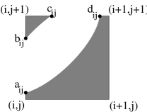
Figure 2: A single cell in the free space

We define an order on the points as follows: For any two points $p_{1}=(x_{1},y_{1}),p_{2}=(x_{2},y_{2})$, $p_{1}\leq p_{2}$ if $x_{1}\leq x_{2}$ and $y_{1}\leq y_{2}$.

Let an $(x,y)$-monotone path be a path that is increasing in both $x$ and $y$ coordinates. Alt and Godau [4] observed that the existence of a $(x,y)$-monotone path in $F_{\varepsilon}$ from $(0,0)$ to $(p,q)$ is a necessary and sufficient condition for $d_{F}(P,Q)\leq\varepsilon$. A similar property holds for $d_{\tilde{F}}$; namely, the existence of any non-self-intersecting path in $F_{\varepsilon}$ from $(0,0)$ to $(p,q)$ implies that $d_{\tilde{F}}(P,Q)\leq\varepsilon$. Denote the property “$(p,q)$ is reachable from $(0,0)$” as property ${\cal P}$ (similarly define $\tilde{\cal P}$).

We wish to solve a decision problem for the Fréchet distance between $P$ and $Q$ minimised over translations i.e given $\varepsilon$, we wish to check whether $\min_{t}d_{F}(P,Q+t)\leq\varepsilon$

The configuration space

A critical event is one that can change the truth value of ${\cal P}$. Each such event is one of the following two types: (1) The intersection points $a_{ij},b_{ij},c_{ij},d_{ij}$ appear (or disappear). (2) For two cells $C_{ij}$ and $C_{kj},k>i$, $a_{ij}$ and $a_{kj}$ (or $b_{kj}$) change their relative vertical ordering. Analogously, for two cells $C_{ij}$ and $C_{ik},k>j$ the points $c_{ij}$ and $c_{ik}$ (or $d_{ik}$) change their relative horizontal ordering.

Type 2 events correspond to the creation or deletion of tunnels. For any point $r$ in the space $[0,p]\times[j,j+1]$, let $k$ be the rightmost interval such that $r$ projected onto the interval $[a_{kj},b_{kj}]$ lies between the endpoints of the interval. We define rt $(r)=k$. For any point $r\in[i,i+1]\times[0,q]$, let $k$ be the topmost interval such that $r$ projected onto the interval $[c_{ik},d_{ik}]$ lies between the endpoints of the interval. We define ut$(r)=k$.

As $Q$ translates, each of the $x_{ij},x\in\{a,b,c,d\}$ can be represented as a function $x_{ij}(t):{\Bbb R}^{2}\rightarrow[0,1]$.

Proposition 4.1

For a point $x_{ij}$, the function $x_{ij}(t)$ is a second degree polynomial in the coordinates of $t$.

From free space to a graph

Our algorithm for computing $d_{F}(P,Q)$ is based on a reduction of the problem to a directed graph reachability problem. Intuitively, we can think of a monotone path in the free space as a path in a directed graph (actually a DAG). The advantage of this approach is that we can exploit known methods for maintaining graph properties dynamically in an efficient manner. Thus, as we traverse the space of translations, we need not recompute the free space at each critical event.

Let $V=\bigcup_{i,j}\{v^{a}_{ij},v^{b}_{ij},v^{c}_{ij},v^{d}_{ij}\}$ and $T=\bigcup_{i,j,i<k\leq p}\{t^{a}_{ijk},t^{b}_{ijk}\}\ \ \cup\ \bigcup_{i,j,j<k\leq q}\{t^{c}_{ijk},t^{d}_{ijk}\}$ where $0\leq i\leq p$ and $0\leq j\leq q$. The vertices in $V\cup T$ are associated with points of the free space. More precisely, vertex $v^{x}_{ij}$ is associated with the point $x_{ij}$ (where $x$ is one of $\{a,b,c,d\}$). Vertex $t^{x}_{ijk}$ is associated with the projection of point $x_{ij}$ onto the interval $[a_{kj},b_{kj}]$ ($x\in\{a,b\}$), and vertex $t^{y}_{ijk}$ is associated with the projection of point $y_{ij}$ onto the interval $[c_{ik},d_{ik}]$ ($y\in\{c,d\}$). We define $f(v)=p$, where $p$ is the point associated with vertex v.

Let $V^{1}_{ij}=\{v^{a}_{ij},v^{b}_{ij}\}\cup\bigcup_{l<i\leq rt(a_{lj})}t^{a}_{lji}\cup\bigcup_{l<i\leq rt(b_{lj})}t^{b}_{lji}$ and $V^{2}_{ij}=\{v^{c}_{ij},v^{d}_{ij}\}\cup\bigcup_{l<j\leq ut(c_{il})}t^{c}_{ilj}\cup\bigcup_{l<j\leq ut(d_{lj})}t^{d}_{ilj}$. $V^{1}_{ij}$ denotes the set of vertices associated with points on the line segment from $(i,j)$ to $(i,j+1)$. Similarly, $V^{2}_{ij}$ denotes the set of vertices associated with points on the line segment from $(i,j)$ to $(i+1,j)$. In addition, $V^{1}_{ij}$ and $V^{2}_{ij}$ contain vertices associated with points whose tunnels cross the cell $C_{ij}$.

We now describe the construction of the edge set for each $(i,j)$. Firstly, set $E^{1}_{ij}=\{(v,v^{b}_{ij})\mid v\in V^{1}_{ij}\}$ and set $E^{2}_{ij}=\{(v,v^{d}_{ij})\mid v\in V^{2}_{ij}\}$ For each $v\in V^{1}_{ij}$, let $n(v)=\arg\min_{v^{\prime}\in V^{1}_{i+1,j},f(v^{\prime})\geq v}f(v^{\prime})$ Similarly, for each $v\in V^{2}_{ij}$, let $n(v)$ denote the vertex in $V^{2}_{i,j+1}$ having the same property. Let $E^{3}_{ij}=\{(v,n(v))\mid v\in V^{1}_{ij}\cup V^{2}_{ij}\}$. Finally, set $E^{4}_{ij}=\{(v^{b}_{ij},v^{c}_{i,j+1}),(v^{d}_{ij},v^{a}_{i+1,j})\}$. Now, we set $E_{ij}=E^{1}_{ij}\cup E^{2}_{ij}\cup E^{3}_{ij}\cup E^{4}_{ij}$.

Let $E=\bigcup_{i,j}E_{ij}$. This yields the directed graph $G=(V\cup T,E)$. Note that $|V\cup T|=O(pq(p+q))$ and $|E|=O(pq(p+q))$. Also, it is easy to see that for any edge $(u,v)\in E$, the straight line from $f(u)$ to $f(v)$ is an $(x,y)$-monotone path. We first show that reachability in the graph $G$ is equivalent to path construction in $F_{\varepsilon}$. The proof of this theorem is straightforward and is deferred to Appendix C.

Theorem 4.2

An $(x,y)$-monotone path from $(0,0)$ to $(p,q)$ exists in $F_{\varepsilon}$ iff $v^{b}_{pq}$ is reachable from $v^{a}_{00}$ and $f(v^{a}_{00})=(0,0),f(v^{b}_{pq})=(p,q)$.

For every edge $e\in E$, let $\gamma(e)\subseteq{\Bbb R}^{2}$ be the set of translations $t$ such that in the graph $G$ constructed from the free space $F_{\varepsilon}(P,Q+t)$, the edge $e$ is present. Let $\Gamma$ be the arrangement of all the $\gamma(e)$. We first establish a bound on the complexity of $\Gamma$.

The following three propositions (which we state without proof), follow from Proposition 4.1. Roughly speaking, with each edge $e$ we can associate a boolean combination of predicates $P_{1},P_{2},\ldots,P_{k}$, where each predicate compares some constant degree polynomial to zero. (i.e the regions are semi-algebraic sets).

$\bullet$ For any region $\gamma(e)$, the boundaries consist of segments of curves described by constant degree polynomials.

$\bullet$ For an edge $e\in E_{ij}-T\times T$, the region $\gamma(e)$ is a constant number of simple regions of constant description complexity.

$\bullet$ For an edge of the form $(t^{x}_{ijk},t^{x}_{ijk+1}),x\in\{a,b,c,d\}$, the region $\gamma(e)$ consists of a set of simple regions of total description complexity $k$.

Lemma 4.3

$|\Gamma|=O(p^{2}q^{2}(p+q)^{4})$.

Proof Sketch: There are $O(pq(p+q))$ edges. For each edge $e$, the complexity of the associated region can be at most $O(p+q)$. Since any pair of constant degree polynomials intersect in a constant number of points, the overall complexity of $\Gamma$ is given by $(pq(p+q)\times(p+q))^{2}$.

 

Lemma 4.4

Let $\gamma_{k}=\gamma((t^{x}_{ijk},t^{x}_{ij,k+1}))$, where $x\in\{a,b,c,d\}$. Then for all $l$ such that $i\leq l<k$, $\gamma_{k}\subseteq\gamma_{l}$.

Proof: Whenever the edge $(t^{x}_{ijk},t^{x}_{ijk+1})$ is present, all edges of the form $(t^{x}_{ij,l},t^{x}_{ijl+1}),i\leq l<k$ must also be present.

 

Theorem 4.2 indicates that the graph property that we need to maintain is the reachability of $v^{b}_{pq}$ from $v^{a}_{00}$. The algorithm is now as follows: Fix a traversal of the arrangement of regions. Check reachability at the starting cell. Each time an edge is crossed in the traversal, it corresponds to the deletion (and insertion) of edges in the graph, which we use to update the graph and check for reachability. Stop whenever the above property holds, returning YES, else return NO.

Theorem 4.5

Iff there exists a translation $t$ such that $d_{F}(P,Q+t)\leq\varepsilon$, the above algorithm will terminate with a YES.

Proof: Consider a type 1 critical event, where the interval $a_{ij},b_{ij}$ is created. This interval corresponds to the edge $(v^{a}_{ij},v^{b}_{ij})$. Hence, this event corresponds to entering the region associated with the above edge. Similar arguments hold for other type 1 critical events.

Suppose we have a type 2 critical event, where the point $a_{kj}$ rises above $a_{ij}$ (in their relative vertical ordering). Note that this event does not change the reachability of $(p,q)$ in the free space unless rt$(a_{ij})>k$. If this is the case, then the event results in setting rt$(a_{ij})=k$, implying that all edges of the form $(t^{a}_{ijl},t^{a}_{ij,l+1}),l\geq k$ are deleted, which corresponds to leaving the regions corresponding to this set of edges.

Conversely, it can be seen that any transition from one cell of the arrangement to another corresponds to a critical event. We defer the details to a full version of the paper.

 

It now remains to analyse the complexity of the above algorithm. A transition between cells yields $O(1)$ updates, except in the case described in Theorem 4.5 above, where a transition occurs across the boundary of region $r((t^{a}_{ij,l-1},t^{a}_{ijl}))$ into the region $r((t^{a}_{ij,k-1},t^{a}_{ijk}))$, causing $\Theta(l-k)$ updates. However, note that in this event, it must be the case that all the regions $r((t^{a}_{ij,m},t^{a}_{ij,m+1}),k\leq m<l-1$ intersect at this transition point (from Lemma 4.4), and thus the cost of this transition can be distributed among these cells. Hence, the total number of updates is given by Lemma 4.3.

To determine reachability, we must now traverse the arrangement. For ease of notation, we will assume that $p=\Theta(q)$ and set $n=p+q$. The arrangement consists of $O(n^{3})$ regions, each described by $O(n)$ curves of constant description complexity. Let us fix $r$ (we will specify the value of $r$ later). It can be shown (using the theory of cuttings [18, 20]) that we can compute a subset ${\cal R}$ of the regions of size $O(r\log r)$ with the property that if we compute the vertical decomposition of each super-cell in the arrangement of ${\cal R}$, each of the resulting primitive super-cells (of constant complexity) is intersected by $O(n^{3}/r)$ regions.

Lemma 4.6

Given a graph $G=(V,E),|V|=N,|E|=M$, designated nodes $s,t\in V$, and a set of $k$ edges $E^{\prime}\subset E$, $s$-$t$ reachability in $G$ can be maintained over edge insertions and deletions from $E^{\prime}$ in total time $O(\min(N^{\omega},Mk)+k^{2}U)$, where $U$ is the number of such updates ($\omega$ is the exponent for matrix multiplication).

Proof: Let $V^{\prime}$ be the set of endpoints of edges in $E^{\prime}$. We compute the graph $G^{\prime}=(V^{\prime\prime}=V^{\prime}\cup\{s,t\},E^{\prime\prime})$, where $(u,v)\in E^{\prime\prime}$ if there is a directed path from $u$ to $v$ in $G$. Note that $|V^{\prime\prime}|\leq 2k$. The computation of this graph can be done by performing a full transitive closure on $G$ that takes time $O(n^{\omega})$. Alternatively, we can perform $O(k)$ depth-first searches (one from each vertex in $V^{\prime\prime}$) to construct $G^{\prime}$.

Now, to process updates, we update the graph using a standard dynamic update procedure that takes time $O(k^{2}\log k)$ time (amortized) per update[25], yielding the result.

 

The algorithm now proceeds as follows: Each primitive super-cell has a set of edges associated with it (one for each region that intersects it). We use the above lemma to perform an efficient dynamic reachability test for each cell of the original arrangement in this primitive super-cell. When we move to the next primitive super-cell, we recompute the induced graph and repeat the process.

We now compute the value of $r$. The total number of cells in the arrangement is $O(n^{8})$ by Lemma 4.3. There are $O(r^{2}n^{2}\log^{2}r)$ primitive super-cells, each intersected by $O(n^{3}/r)$ regions. Consider a single primitive super-cell $i$. We apply Lemma 4.6 with $N=M=O(n^{3})$, $k=O(n^{3}/r)$, and $U=U_{i}$, where $U_{i}$ is the number of cells in $i$. The current value of $\omega$ is approximately $2.376$ [19], and thus $\min(N^{\omega},Mk)=Mk=n^{6}/r$ for all $r=\Omega(1)$. The cost of processing $i$ is therefore $n^{6}/r$ + $n^{6}U_{i}/r^{2}$. Summing over all primitive super-cells, and replacing $\Sigma U_{i}$ by $O(n^{8})$, we obtain the overall running time of the algorithm to be $O(n^{8}r\log^{2}r+n^{14}/r^{2})$. Balancing, we obtain an overall running time of $O(n^{10}\mbox{\sl polylog}\,n)$.

Theorem 4.7

Given two polygonal chains $P,Q,|P|=p,|Q|=q$, and $\varepsilon>0$, we can check if $d_{F}(P,Q)\leq\varepsilon$ in time $O(n^{10}\mbox{\sl polylog\,}n)$.

The weak Fréchet distance 

As described earlier, the weak Fréchet distance (denoted by $d_{\tilde{F}}$) relaxes the constraint that the parametrizations employed must be monotone. Note that for any two curves $P,Q$, the following inequality is true: $d_{H}(P,Q)\leq d_{\tilde{F}}(P,Q)\leq d_{F}(P,Q)$ Also, by the result of Godau [21], all three measures collapse to one if both curves are convex. The above inequality is significant because it suggests that the weak Fréchet distance may serve as a relaxed curve matching measure with possibly more tractable algorithms.

As it turns out, this is indeed the case. Our techniques from the previous algorithm apply here as well, with two key differences. Firstly, since the paths need not be monotone, we no longer need the concept of a tunnel, thus reducing the number of critical events that need to be examined to $O(pq)$. Secondly, the underlying graph is now undirected, and there are efficient procedures for maintaining connectivity in an undirected graph [23]. We defer details to a full version of the paper, and summarize the result as:

Theorem 4.8

Given two polygonal chains $P,Q,|P|=p,|Q|=q$, and $\varepsilon>0$, we can check if $\min_{t}d_{F}(P,Q+t)\leq\varepsilon$ in time $O(n^{4}\mbox{\sl polylog\,}n)$, where $n=O(p+q)$.

An approximation scheme

An $(\varepsilon,\beta)$-approximation (defined by Heffernan and Schirra [22]) for $d_{F}(P,Q)$ under translations can be obtained from the following observation:

Lemma 4.9

Given polygonal chains $P,Q$, let $t$ be the translation that maps the first point of $Q$ to the first point of $P$. Then $d_{F}(P,Q+t)\leq 2d^{*}$, where $d^{*}=\min_{\mbox{translations\ }t}d_{F}(P,Q+t)$.

Proof: Let $t^{*}$ be the translation such that $d_{F}(P,Q+t^{*})=d^{*}$. Clearly, the first point in $Q$ is at most $d^{*}$ away from the first point of $P$. Applying the translation $t^{\prime}=t-t^{*}$ to $Q$, no point in $Q$ is moved more than $d^{*}$ units away from its associated point in $P$. Hence, $d_{F}(P,Q+t^{*}+t^{\prime})=d_{F}(P,Q+t)\leq 2d^{*}$.

 

Applying the standard discretization trick in a ball of radius $d^{*}$ around the first point of $P$, we obtain an $(\varepsilon,\beta)$-approximation for any $\beta>0$. Note that this scheme is very efficient, running in time $O(n^{2}{{\sl poly}}(\log n$, $1/\beta))$.

Appendix A Proof of Lemma 2.1

Definition A.1

For a geometric object $R$ let $X(R)$, the $x$-span of $R$, denote the interval of the $x$-axis between the leftmost and the rightmost point of $R^{\prime}$, where $R^{\prime}$ is the orthogonal projection of $R$ on the $x$-axis.

Claim A.2

Let $P=\{(x_{1},y_{1}),\dots(x_{m},y_{m})\}$ be a point set. We can construct in time $O(m\log^{2}m)$ a data structure for $P$ such that given a query segment $s$, the point $(x_{k},y_{k})$ that maximizes the $y$-value of the set $\{s(x_{i})+y_{i}~{}|~{}x_{i}\in X(s),1\leq i\leq m\}$ can be found in time $O(\log^{2}m)$.

Proof: If $X(P)\subseteq X(s)$, then $(x_{k},y_{k})$ is clearly a vertex of the convex hull of $P$, and once the convex hull is computed, we can find $(x_{k},y_{k})$ in time $O(\log n)$. To answer the query in the case that $X(P)$ is not contained in $X(s)$, we construct a sorted balanced binary tree $\Psi=\Psi(P)$ on the set $\{x_{1}\dots x_{m}\}$. For each node $\mu\in\Psi$ let $P_{\mu}$ denote the points in the subtree of $\mu$, and let $X_{\mu}$ denote the $x$-span of $P_{\mu}$. We construct $C_{\mu}$, the convex hull of $P_{\mu}$, for each node $\mu$ of $\Psi$. Once a query segment $s$ is given, we find a set $U$ of $O(\log|P|)$ nodes of $\Psi$ with the property that for each node $\mu\in U$, $X_{\mu}$ is contained in $X(s)$, and in addition, each $(x_{i},y_{i})\in P$ for which $x_{i}\in X(s)$ appears in exactly one of the sets $P_{\mu}$, for $\mu\in U$. We perform the query suggested by the previous claim on $C_{\mu}$ for each $\mu\in U$.

 

Based on Claim A.2, we describe the data structure as follows. Let $m=|{\cal S}|$. First observe that the maximum must be obtained at an endpoint of a segment of ${\cal S}$. We partition ${\cal S}$ into ${\cal S}_{1}$ and ${\cal S}_{2}$. The set ${\cal S}_{2}$ contains at least $m-\sqrt{m}$ of the segment of ${\cal S}$. It is updated after $\sqrt{m}$ insertions or deletion operations into/from ${\cal S}$ Once it is updated, we explicitly compute the function $\mbox{\sl sum}_{{\cal S}_{1}}(\cdot)$, and construct the data structure $\Psi=\Psi_{{\cal S}_{1}}$ of Claim A.2 for the vertices of the graph of $\mbox{\sl sum}_{{\cal S}_{1}}(\cdot)$. As easily observed, the complexity of the graph of $\mbox{\sl sum}_{{\cal S}_{1}}(\cdot)$ is $O(m)$, since a vertex of this function occurs only at endpoint of a segment of ${\cal S}_{1}$, thus the time needed to constuct $\Psi=\Psi_{{\cal S}_{1}}$. The set ${\cal S}_{2}={\cal S}\setminus{\cal S}_{1}$ has cardinality $\leq\sqrt{m}$. Each time a segment is inserted (resp. deleted) into/from ${\cal S}$, it is inserted (resp. deleted) into/from ${\cal S}_{1}$. Once the size of ${\cal S}_{1}$ exceeds $\sqrt{m}$, we set ${\cal S}_{1}$ to be ${\cal S}$, construct $\Psi$, and empty ${\cal S}_{2}$.

In order to maintain the maximum $\max(\mbox{\sl sum}_{\cal S}(\cdot))$, we do the following. Once a segment is inserted or deleted into ${\cal S}_{1}$, we explicitly compute (the graph of) $\mbox{\sl sum}_{\cal S}(\cdot)$ which is piecewise linear of complexity $O(\sqrt{m})$. With each segment $e$ of this graph (not to be confused with the segments of ${\cal S}$) we perform a query in $\Psi_{{\cal S}_{1}}$. The maximum obtained is is $\max(\mbox{\sl sum}_{\cal S}(\cdot))$.

Next we describe the modifications of the data structure needed in the case where (some of) the segments of ${\cal S}$ move vertially in a constant speed with the time parameter $\tau$. Let $X^{\prime}=\{x_{1}\dots x_{m}\}$ denote the $x$-coordinates of the endpoints of the segments of ${\cal S}$. They are not time dependent. Let $y(x,\tau)$ denote the $y$-value of the sum function at the coordination $x$ at time $\tau$. Clearly as long as no insertions or deletions are taken place in ${\cal S}$, $y(x,\tau)$ moves (vertically) at a constant velocity. It is well known fact that the convex hull of such a set of points can go through $O(m)$ combinatorial changes, which we can compute in time $O(m\log m)$. This suggest the following modification to the data structure of ${\cal T}$ as follows. As before, each node $\mu$ is associated as before with the convex hull $C_{\mu}=C_{\mu}(t)$, but now these convex hulls might change in time. However, as argued, the total number of changes they go through is only $O(m\log^{2}m)$. The query process remains the same.

Appendix B Proof of Theorem 2.4

Assume for the construction that $\varepsilon=1/2$. The first component in the construction (see Figure 3) is the set $B_{1}^{\prime}$ consisting of $2n$ points, which are

$$\{(i,{1/2}-i/n)\mbox{ ~{} and ~{}}(i,-{1/2}-i/n-1/4n^{2}),~{}~{}\mbox{for}i=1\dots n\}\ .$$

Thus the $i^{th}$ pair $(i,{1/2}-i/n)^{+}\mbox{ ~{} and ~{}}(i,-{1/2}-i/n-\delta)^{+}$ (i.e., the Minkowski sum of these points and the $\ell_{i}nfty$ ball) form two close vertically aligned squares, where the gap between them is of unit width, and of height $1/4n^{2}$. The $i^{th}$ pair is located at distance $i/n$ below the $x$-axis. We add the segment $B_{1}^{\prime\prime}$, which is the long horizontal segment between the points $(-n,-1/4)$ and $(0,-1/4)$ and the segment $B_{1}^{\prime\prime\prime}$ between $(n,-1/4)$ and $(2n,-1/4)$. Let $B_{1}=B_{1}^{\prime}\cup B_{1}^{\prime\prime}\cup B_{1}^{\prime\prime\prime}$.

Figure 3: The lower bound construction for $n=3$. The set $B$ is not shown explicitly; only $B^{+}$ is shown.

The set $A_{1}$ consists of $n$ horizontal segments of length $2n$, each separated by a gap of $1/n^{2}$ from the next one. The left endpoint of all of them is on the $y$-axis, and the middle one is on the $x$-axis. By shifting them vertically, each segment in turn is not completely covered at some time, when it passes between the gaps between one of the pairs of $B_{1}$. In all other cases, all the segments are completely covered. The region in TP  corresponds to all translations $t$ for which $h(t+A_{1},B_{1})\leq 1$ consists of $\Omega(n^{2})$ horizontal strips, each of length $n$.

The set $B_{2}$ consists of the $n$ points $(-(1+1/n^{2})i,-5)$ (for $i=1\dots n$). Thus $B_{2}^{+}$ creates $n$ unit squares along the line $y=-5$, with a gap of $1/n^{2}$ between them. The set $A_{1}$ consist of $n$ points along the horizontal line $(-1/2n,-5)$ (for $i=1\dots n$). Observe that $A_{1}$ fits completely into each of the squares of $B_{2}^{+}$. However, by sliding $A_{1}$ horizontally, along $y=-5$ or anywhere at distance $\leq 1$ from $h$, each of the points of $A_{1}$ “falls” at some stage into each of the gaps between each of the squares of $B_{2}^{+}$, The region $S_{2}=\{t\,|\,h(t+A_{2},B_{2})\leq 1\}$ consists of $\Omega(n^{2})$ vertical strips in TP , each of hight $2$. Letting $A=A_{1}\cup A_{2}$ and $B=B_{1}\cup B_{2}$, the region $S=\{t\,|\,h(t+A,B)\leq 1\}$ is merely the intersection of $S_{1}$ and $S_{2}$, which is clearly of complexity $\Omega(n^{4})$, thus proving our claim.

Appendix C Proof of Theorem 4.2

Suppose $v^{b}_{pq}$ is reachable from $v^{a}_{00}$ and $f(v^{a}_{00})=(0,0),f(v^{b}_{pq})=(p,q)$. Let the path in $G$ be $v_{1}=v^{a}_{00},v_{2},\ldots,v_{k}=v^{b}_{pq}$. Replace each vertex $v_{i}$ by its associated point $f(v_{i})$. As observed above, if we now connect the points $f(v_{1}),f(v_{2}),\ldots,f(v_{k})$ by straight lines, we obtain an $(x,y)$-monotone path.

Conversely, suppose there exists an $(x,y)$-monotone path $w$ from $(0,0)$ to $(p,q)$ in $F_{\varepsilon}$. Then $(0,0)\in C_{00}$ and $(p,q)\in C_{p-1,q-1}$ and thus $f(v^{a}_{00})=(0,0)$ and $f(v^{b}_{pq})=(p,q)$. Without loss of generality, we can assume that $w$ consists of a sequence of line segments, where the endpoints of each segment are one of the $x_{ij}$’s ($x=\{a,b,c,d\}$).

We will show by induction on the number of segments that $v^{b}_{pq}$ is reachable from $v^{a}_{00}$. Assume that the claim holds for the first $k$ segments on the path. Consider the $(k+1)^{th}$ segment. Let the endpoints be $w_{1},w_{2}$. By the induction hypothesis, $w_{1}$ is reachable from $v^{a}_{00}$.

Case 1: Let both $w_{1},w_{2}$ be of the form $x_{ij},y_{kj}$ respectively, where $x,y\in\{a,b\}$. If rt$(f(w_{1}))\geq k$, then the vertex $t^{x}_{ijl}$ exists for all $l\leq k$, and thus there exists a path $w_{1},t^{x}_{ij,i+1},\ldots,t^{x}_{ijk}$. Since $f(t^{x}_{ijk})$ is on the same interval as $f(w_{2})$ and must be below it, there exists an edge from $t^{x}_{ijk}$ to $w_{2}$ in $E_{2}$ . If on the other hand, rt$(f(w_{1}))<k$, there must exist one vertex $w^{\prime}=x^{lj},i<l<k$ such that $f(w^{\prime})>f(w_{1})$, and rt$(f(w_{1})\leq l$. We construct a path from $w_{1}$ to $w^{\prime}$ and repeat.

Case 2: Let both $w_{1}$ and $w_{2}$ be of the form $x_{ij},y_{ik}$ respectively, where $x,y\in\{c,d\}$. An argument similar to Case 1 applies here.

Case 3: Let $w_{1}=a_{ij}$ and $w_{2}=d_{kl}$. Without loss of generality we can assume that $k=i$ and $l=j+1$. There exists an edge from $v^{a}_{ij}$ to $v^{b}_{ij})$, which is a predecessor of $v^{c}_{i,j+1})$ (using $E_{4}$), and there exists an edge from $v^{c}_{i,j+1})$ to $v^{d}_{kl}$, thus yielding the desired path. Other cases can be handled symmetrically.

Thus, by induction the theorem holds.

References

- [1]
- [2] K. Abrahamson, Generalized string matching, SIAM Journal on Computing, 16 (1987), 1039–51.
- [3] Pankaj K. Agarwal and Micha Sharir and S. Toledo, Applications of parametric searching in geometric optimization, J. Algorithms, 17 (1994), 292–318.
- [4] H. Alt and M. Godau Computing the Fréchet distance between two polygonal curves, International J. of Computational Geometry and Applications 5 (1995), 75–91.
- [5] A. Amir, M. Farach, Efficient 2-dimensional approximate matching of half-rectangular figures, Information and Computation, 118 (1995), 1–11.
- [6] Gill Barequet and Sariel Har-Peled, Some Variants of Polygon Containment and Minimum Hausdorff Distance under Translation are 3sum-Hard, Proceedings Annual ACM-SIAM Symposium on Discrete Algorithms1999.
- [7] D. Cardoze, L. Schulman, Pattern Matching for Spatia l Point Sets, Proc. 39th FOCS, 1998.
- [8] L.P. Chew and K. Kedem, Improvements on geometric pattern matching problems, Proceedings 3rd Scand. Workshop on Algorithms Theory, LNCS #621, 1992, 318–325.
- [9] L.P. Chew, D. Dor, A. Efrat, and K. Kedem, Geometric Pattern Matching in -Dimensional Space, Proceedings of the 3rd European Symposium on Algorithms (ESA) LNCS #979, 1995, 264–279. Also in Discrete and Computational Geometry, to appear.
- [10] L.P. Chew, M.T. Goodrich, D.P. Huttenlocher, K. Kedem, J. M. Kleinberg, and D. Kravets, Geometric pattern matching under Euclidean motion, Computational Geometry: Theory and Applications 7 (1997), 113-124.
- [11] M. Fréchet, Sur quelques points du calcul fonctionnel, Rendiconti del Circolo Mathematico di Palermo 22 (1906), 1–74.
- [12] P. Indyk, R. Motwani, S. Venkatasubramanian, Geometric Matching Under Noise: Combinatorial Bounds and Algorithms, 10th Symposium on Discrete Algorithms (SODA), 1999.
- [13] K. Kedem, R. Livne, J. Pach, M. Sharir, On the union of Jordan regions and collision-free translational motion amidst polygonal obstacles, Discrete and Computational Geometry 1 (1986), 59–71.
- [14] S. R. Kosaraju, Efficient string matching. manuscript, 1987.
- [15] W. Rucklidge, Lower Bounds for the Complexity of the Hausdorff Distance, Proceedings 5Candian Conf. Computational Geometry 1993, 145–150.
- [16] H. Alt, J. Blömer, M. Godau, and H. Wagener. Approximation of convex polygons. In Proc. 17th International Colloquium on Automata, Languages and Programming, volume 443 of LNCS , 703–716. Springer-Verlag, 1990.
- [17] P. Bogacki and S. Weinstein. Generalized fréchet distance between curves. In M. Daehlen, T. Lyche, and L. L. Schumaker, editors, Mathematical Methods for Curves and Surfaces II, 25–32. Vanderbilt University Press, 1998.
- [18] Bernard Chazelle. Cutting hyperplanes for divide-and-conquer. Discrete Comput. Geom., 9(2):145–158, 1993.
- [19] D. Coppersmith and S. Winograd. Matrix multiplication via arithmetic progressions. Journal of Symbolic Computation, 9:1–6, 1990.
- [20] M. de Berg and O. Schwarzkopf. Cuttings and applications. Internat. J. Comput. Geom. Appl., 5:343–355, 1995.
- [21] Michael Godau. On the complexity of measuring the similarity between geometric objects in higher dimensions. PhD thesis, Department Mathematik u. Informatik, Freie Universit t Berlin, December 1998.
- [22] P. J. Heffernan and S. Schirra. Approximate decision algorithms for point set congruence. Computational Geometry: Theory and Applications, 4(3):137–156, 1994.
- [23] J. Holm, K. Lichtenberg, and M. Thorup. Poly-logarithmic deterministic fully-dynamic algorithms for connectivity, minimum spanning tree, 2-edge and biconnectivity. In Proc. 30th ACM Symposium on Theory of Computing, pages 79–89. ACM, 1998.
- [24] S. Khanna, R. Motwani, and R. Wilson. On certificates and lookahead in dynamic graph problems. Algorithmica, 21(4):377–394, 1998.
- [25] V. King. Fully dynamic algorithms for maintaining all-pairs shortest paths and transitive closure in digraphs. In Proc. 40th IEEE Symposium on Foundations of Computer Science. IEEE, October 1999.
- [26] S. Venkatasubramanian. Geometric Shape Matching and Drug Design. PhD thesis, Department of Computer Science, Stanford University, August 1999.
- [27] A. Winzen and H. Niemann. Matching and fusing 3D-polygonal approximations for model generation. In Proc. IEEE International Conference on Image Processing, volume 1, pages 228–232, Austin, Texas, 1994.