Computing Crossing Numbers in Quadratic Time

Abstract

We show that for every fixed $k\geq 0$ there is a quadratic time algorithm that decides whether a given graph has crossing number at most $k$ and, if this is the case, computes a drawing of the graph in the plane with at most $k$ crossings.

1 Introduction

Hopcroft and Tarjan [13] showed in 1974 that planarity of graphs can be decided in linear time. It is natural to relax planarity by admitting a small number of edge-crossings in a drawing of the graph. The crossing number of a graph is the minimum number of edge crossings needed in a drawing of the graph in the plane. Not surprisingly, it is NP-complete to decide, given a graph $G$ and a $k$, whether the crossing number of $G$ is at most $k$ [12]. On the other hand, for every fixed $k$ there is a simple polynomial time algorithm deciding whether a given graph $G$ has crossing number at most $k$: It guesses $l\leq k$ pairs of edges that cross and tests if the graph obtained from $G$ by adding a new vertex at each of these edge crossings is planar. The running time of this algorithm is $n^{\Theta(k)}$. Downey and Fellows [6] raised the question if the crossing-number problem is fixed parameter-tractable, that is, if there is a constant $c\geq 1$ such that for every fixed $k$ the problem can be solved in time $O(n^{c})$. We answer this question positively with $c=2$. In other words, we show that for every fixed $k$ there is a quadratic time algorithm deciding whether a given graph $G$ has crossing number at most $k$. Moreover, we show that if this is the case, a drawing of $G$ in the plane with at most $k$ crossings can also be computed in quadratic time.

It is interesting to compare our result to similar results for computing the genus of a graph. (The genus of a graph $G$ is the minimum taken over the genus of all surfaces $S$ such that $G$ can be embedded into $S$.) As for the crossing number, it is NP-complete to decide if the genus of a given graph is less than or equal to a given $k$ [17]. For a fixed $k$, at first sight the genus problem looks much harder. It is by no means obvious how to solve it in polynomial time; this has been proved possible by Filotti, Miller, and Reif [10]. In 1996, Mohar [14] proved that for every $k$ there is actually a linear time algorithm deciding whether the genus of a given graph is $k$. However, the fact that the genus problem is fixed-parameter tractable was known earlier as a direct consequence of a strong general theorem due to Robertson and Seymour [16] stating that all minor closed classes of graphs are recognizable in cubic time. It is easy to see that the class of graphs of genus at most $k$ is closed under taking minors, but unfortunately the class of all graphs of crossing number at most $k$ is not. So in general Robertson and Seymour’s theorem cannot be applied to compute crossing numbers. An exception is the case of graphs of degree at most 3; Fellows and Langston [8] observed that for such graphs Robertson and Seymour’s result immediately yields a cubic time algorithm for computing crossing numbers.

Although we cannot apply Robertson and Seymour’s result directly, the overall strategy of our algorithm is inspired by their ideas: The algorithm first iteratively reduces the size of the input graph until it reaches a graph of bounded tree-width, and then solves the problem on this graph. For the reduction step, we use Robertson and Seymour’s Excluded Grid Theorem [15] together with a nice observation due to Thomassen [18] that in a graph of bounded genus (and thus in a graph of bounded crossing number) every large grid contains a subgrid that, in some precise sense, lies “flat” in the graph. Such a flat grid does not essentially contribute to the crossing number and can therefore be contracted. For the remaining problem on graphs of bounded tree-width we apply a theorem due to Courcelle [3] stating that all properties of graphs that are expressible in monadic second-order logic are decidable in linear time on graphs of bounded tree-width.

Let me remark that the hidden constant in the quadratic upper bound for the running time of our algorithm heavily depends on $k$. As a matter of fact, the running time is $O(f(k)\cdot n^{2})$, where $f$ is a doubly exponential function. Thus our algorithm is mainly of theoretical interest.

2 Preliminaries

Graphs in this paper are undirected and loop-free, but they may have multiple edges. The vertex set of a graph $G$ is denoted by $V^{G}$, the edge set by $E^{G}$. For graphs $G$ and $H$ we let $G\cup H:=(V^{G}\cup V^{H},E^{G}\cup E^{H})$ and $G\setminus H:=\big{(}V^{G}\setminus V^{H},\{e\in E^{G}\setminus E^{H}\mid\text{both endpoints of $e$ are contained in $V^{G}\setminus V^{H}$}\}\big{)}$.

2.1 Topological Embeddings

A topological embedding of a graph $G$ into a graph $H$ is a mapping $h$ that associates a vertex $h(v)\in V^{H}$ with every $v\in V^{G}$ and a path $h(e)$ in $H$ with every $e\in E^{G}$ in such a way that:

• For distinct vertices $v,w\in V^{G}$, the vertices $h(v)$ and $h(w)$ are distinct.

• For distinct edges $e,f\in E^{G}$, the paths $h(e)$ and $h(f)$ are internally disjoint (that is, they have at most their endpoints in common).

• For every edge $e\in E^{G}$ with endpoints $v$ and $w$, the two endpoints of the path $h(e)$ are $h(v)$ and $h(w)$, and $h(u)\not\in V^{h(e)}$ for all $u\in V^{G}\setminus\{v,w\}$.

We let $h(G):=\big{(}h(V^{G}),\emptyset\big{)}\cup\bigcup_{e\in E^{G}}h(e)$.

2.2 Drawings and Crossing Numbers

A drawing of a graph $G$ is a mapping $\Delta$ that associates with every vertex $v\in V^{G}$ a point $\Delta(v)\in\mathbb{R}^{2}$ and with every edge $e\in E^{G}$ a simple curve $\Delta(e)$ in $\mathbb{R}^{2}$ in such a way that:

• For distinct vertices $v,w\in V^{G}$, the points $\Delta(v)$ and $\Delta(w)$ are distinct.

• For distinct edges $e,f\in E^{G}$, the curves $\Delta(e)$ and $\Delta(f)$ have at most one interior point in common (and possibly their endpoints).

• For every edge $e\in E^{G}$ with endpoints $v$ and $w$, the two endpoints of the curve $\Delta(e)$ are $\Delta(v)$ and $\Delta(w)$, and $\Delta(u)\not\in\Delta(e)$ for all $u\in V^{G}\setminus\{v,w\}$.

• At most two edges intersect in one point. More precisely, $|\{e\in E^{G}\mid x\in\Delta(e)\}|\leq 2$ for all $x\in\mathbb{R}^{2}\setminus\Delta(V^{G})$.

We let $\Delta(G):=\Delta(V^{G})\cup\bigcup_{e\in E^{G}}\Delta(e)$.

An $x\in\mathbb{R}^{2}\setminus\Delta(V^{G})$ with $|\{e\in E^{G}\mid x\in\Delta(e)\}|=2$ is called a crossing of $\Delta$. The crossing number of $\Delta$ is the number of crossings of $\Delta$. The crossing number of $G$ is the minimum taken over the crossing numbers of all drawings of $G$. A drawing or graph of crossing number 0 is called planar.

2.3 Hexagonal Grids

For $r\geq 1$, we let $H_{r}$ be the hexagonal grid of radius $r$. Instead of giving a formal definition, we refer the reader to Figure 1 to see what this means.

Figure 1: The hexagonal grids $H_{1},H_{2},H_{3}$

The principal cycles $C_{1},\ldots,C_{r}$ of $H_{r}$ are the the concentric cycles, numbered from the interior to the exterior (see Figure 2).

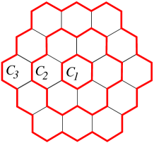
Figure 2: The principal cycles of $H_{3}$

2.4 Flat Grids in a Graph

For graphs $H\subseteq G$, an $H$-component (of $G$) is either a connected component $C$ of $G\setminus H$ together with all edges connecting $C$ with $H$ and their endpoints in $H$ or an edge in $E^{G}\setminus E^{H}$ whose endpoints are both in $H$ together with its endpoints. Let $G$ be a graph and $h:H_{r}\to G$ a topological embedding. The interior of $h(H_{r})$ is the subgraph $h(H_{r}\setminus C_{r})$ (remember that $C_{r}$ is the outermost principal cycle of $H_{r}$). The attachments of $h(H_{r})$ are those $h(H_{r})$-components that have a non-empty intersection with the interior of $h(H_{r})$. The topological embedding $h$ is flat if the union of $h(H_{r})$ with all its attachments is planar.

We shall use the following theorem due to Thomassen [18]. Actually, Thomassen stated the result for the genus of a graph rather than its crossing number. However, it is easy to see that the crossing number of a graph is an upper bound for its genus.

• For all $k,r\geq 1$ there is an $s\geq 1$ such that the following holds: If $G$ is a graph of crossing number at most $k$ and $h:H_{s}\to G$ a topological embedding, then there is a subgrid $H_{r}\subseteq H_{s}$ such that the restriction $h|_{H_{r}}$ of $h$ to $H_{r}$ is flat.

2.5 Tree-Width

We assume that reader is familiar with the notion tree-width (of a graph). It is no big problem if not; we never really work with tree-width, but just take it as a black box in Theorems Theorem 2.2 (Robertson, Seymour [16], Bodlaender [1]).–Theorem 2.4.. Robertson and Seymour’s deep Excluded Grid Theorem [15] states that every graph of sufficiently large tree-width contains the homeomorphic image of a large grid. The following is an algorithmic version of this theorem.

• Let $r\geq 1$. Then there is a $w\geq 1$ and a linear time algorithm that, given a graph $G$, either (correctly) recognizes that the tree-width of $G$ is at most $w$ or computes a topological embedding $h:H_{r}\to G$.

Actually, in [16] Robertson and Seymour only give a quadratic time algorithm, but they point out that their algorithm can be improved to linear time using Bodlaender’s [1] linear time algorithm for computing tree-decompositions. Let me remark that, as far as I can see, this algorithm is not merely a trivial modification of Robertson and Seymour’s algorithm obtained by “plugging in” Bodlaender’s tree-decomposition algorithm, but it requires to look into the details of Bodlaender’s algorithm and extend it in a suitable way.

2.6 Courcelle’s Theorem

Courcelle’s theorem states that properties of graphs definable in Monadic Second-Order Logic MSO can be checked in linear time. In this logical context we consider graphs as relational structures of vocabulary $\{E,V,I\}$, where $V$ and $E$ are unary relation symbols interpreted as the vertex set and edge set, respectively, and $I$ is a binary relation symbol interpreted by the incidence relation of a graph. To simplify the notation, for a graph $G$ we let $U^{G}:=V^{G}\cup E^{G}$ and call $U^{G}$ the universe of $G$.

I assume that the reader is familiar with the definition of MSO. However, for those who are not I have included it in Appendix A.

• Let $w\geq 1$ and let $\varphi(x_{1},\ldots,x_{k},X_{1},\ldots,X_{l})$ be an MSO-formula. Then there is a linear time algorithm that, given a graph $G$ and $a_{1},\ldots,a_{k}\in U^{G}$, $A_{1},\ldots,A_{l}\subseteq U^{G}$, decides whether $G\models\varphi(a_{1},\ldots,a_{k},A_{1},\ldots,A_{l})$.

We shall also use the following strengthening of Courcelle’s theorem, a proof of which can be found in [11]:

• Let $w\geq 1$ and let $\varphi(x_{1},\ldots,x_{k},X_{1},\ldots,X_{l},y_{1},\ldots,y_{m},Y_{1},\ldots,Y_{n})$ be an MSO-formula. Then there is a linear time algorithm that, given a graph $G$ and $b_{1},\ldots,b_{m}\in U^{G}$, $B_{1},\ldots,B_{n}\subseteq U^{G}$, decides if there exist $a_{1},\ldots,a_{k}\in U^{G}$, $A_{1},\ldots,A_{l}\subseteq U^{G}$ such that

  $$G\models\varphi(a_{1},\ldots,a_{k},A_{1},\ldots,A_{l},b_{1},\ldots,b_{m},B_{1},\ldots,B_{n}),$$

  and, if this is the case, computes such elements $a_{1},\ldots,a_{k}$ and sets $A_{1},\ldots,A_{l}$.

3 The Algorithm

For an $l\geq 1$, a graph $G$, and a subset $F\subseteq E^{G}$ of forbidden edges, an $l$-good drawing of $G$ with respect to $F$ is a drawing $\Delta$ of $G$ of crossing number at most $l$ such that no forbidden edges are involved in any crossings, i.e. for every crossing $x\in\Delta(e)\cap\Delta(f)$ of $\Delta$ we have $e,f\in E^{G}\setminus F$.

We fix a $k\geq 1$ for the whole section. We shall describe an algorithm that solves the following generalized $k$-crossing number problem in quadratic time:

Input: Graph $G$ and subset $F\subseteq E^{G}$. Problem: Decide if $G$ has a $k$-good drawing with respect to $F$.

Later, we shall extend our algorithm in such a way that it actually computes a $k$-good drawing if there exists one.

Our algorithm works in two phases. In the first, it iteratively reduces the size of the input graph until it obtains a graph whose tree-width is bounded by a constant only depending on $k$. Then, in the second phase, it solves the problem on this graph of bounded tree-width.

Phase I

We let $r:=2k+2$ and choose $s$ sufficiently large such that for every graph $G$ of crossing number at most $k$ and every topological embedding $h:H_{s}\to G$ there is a subgrid $H_{r}\subseteq H_{s}$ such that the restriction $h|_{H_{r}}$ of $h$ to $H_{r}$ is flat. Such an $s$ exists by Theorem Theorem 2.1 (Thomassen [18]).. Then we choose $w$ with respect to $s$ according to Theorem Theorem 2.2 (Robertson, Seymour [16], Bodlaender [1]). such that we have a linear time algorithm that, given a graph of tree-width at least $w$, finds a topological embedding $h:H_{s}\to G$. We keep $r,s,w$ fixed for the rest of the section.

• There is a linear time algorithm that, given a graph $G$, either recognizes that the crossing number of $G$ is greater than $k$, or recognizes that the tree-width of $G$ is at most $w$, or computes a flat topological embedding $h:H_{r}\to G$.

Proof: We first apply the algorithm of Theorem Theorem 2.2 (Robertson, Seymour [16], Bodlaender [1]).. If it recognizes that the tree-width of the input graph $G$ is at most $w$, we are done. Otherwise, it computes a topological embedding $h:H_{s}\to G$. By our choice of $s$, we know that either the crossing number of $G$ is greater than $k$ or there is a subgrid $H_{r}\subseteq H_{s}$ such that the restriction of $h$ to $H_{r}$ is flat.

For each $H_{r}\subseteq H_{s}$ we can decide whether $h|_{H_{r}}$ is flat by a planarity test, which is possible in linear time [13]. Our algorithm tests whether $h|_{H_{r}}$ is flat for all $H_{r}\subseteq H_{s}$. Either it finds a flat $h|_{H_{r}}$, or the crossing number of $G$ is greater than $k$.

Since $s$ is a fixed constant, the overall running time is linear. $\Box$

Let $G$ be a graph and $h:H_{r}\to G$ a flat topological embedding. For $2\leq i\leq r$, we let $H^{i}$ be the subgrid of $H_{r}$ bounded by the $i$th principal cycle $C_{i}$. We let $K_{i}$ be the subgraph of $G$ consisting of $h(H^{i})$ and all attachments of $h(H_{r})$ intersecting the interior $h(H^{i}\setminus C_{i})$ of $h(H_{i})$. Moreover, we let $F_{i}$ be the set of all edges of $K_{i}$ that have at least one endpoint on $h(C_{i})$. Using the fact that $h$ is flat, it is easy to see that the sets $F_{i}$, for $2\leq i\leq r$ are disjoint.

Suppose now that $\Delta$ is a $k$-good drawing of $G$ of minimum crossing number. Recall that $r=2k+2$. By the pigeonhole-principle there is at least one $i,2\leq i\leq r$ such that none of the edges in $F_{i}$ is involved in any crossing of $\Delta$. We let $i_{0},2\leq i\leq r$ be minimum with this property.

Let $C:=h(C_{i_{0}})$, $K:=K_{i_{0}}$ and $I:=K\setminus C$. Then $K$ and $I$ are both connected planar graphs. Note furthermore that $\Delta(C)$ is a simple closed curve in the plane $\mathbb{R}^{2}$. Thus $\Delta(I)$ must be entirely contained in one connected component of $\mathbb{R}^{2}\setminus\Delta(C)$, say, in the interior.

I claim that the restriction of $\Delta$ to $K$ is a planar drawing. Suppose for contradiction that this is not the case. Consider any planar drawing $\Pi$ of $K$. Then $\Pi(C)$ is a simple closed curve in the plane, and without loss of generality we can assume that $\Pi(I)$ is entirely contained in the interior of $\mathbb{R}^{2}\setminus\Pi(C)$. Now we define a new drawing $\Delta^{\prime}$ of $G$ that is identical with $\Delta$ on $G\setminus I$ and homeomorphic to $\Pi$ on $K$. Since none of the edges in $F_{i}$ is involved in any crossing of $\Delta$, this can be done in such a way that none of the edges in $F_{i}$ is involved in any crossing of $\Delta^{\prime}$. But then the number of crossings of $\Delta^{\prime}$ is smaller than that of $\Delta$, because the restricion of $\Delta^{\prime}$ to $K$ is planar. This contradicts the minimality of the crossing number of $\Delta$.

Hence the restriction of $\Delta$ to $K$ is planar. In particular, this means that none of the edges of $F_{2}$ is involved in any crossing of $\Delta$. By the minimality of $i_{0}$, this implies $i_{0}=2$. Thus, surprisingly, $i_{0}$ is independent of the drawing $\Delta$.

Let $G^{\prime}$ be the graph obtained from $G$ by contracting the connected subgraph $I$ to a single vertex $v_{I}$ (see Figure 3).

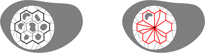
Figure 3: The transformation from a graph $G$ to $G^{\prime}$

Let $F^{\prime}$ be the union of $F$ with the set of all edges of $h(C)$ and all edges incident with the new vertex $v_{I}$. Then $G$ has a $k$-good drawing with respect to $F$ if, and only if, $G^{\prime}$ has a $k$-good drawing with respect to $F^{\prime}$. The forward direction of this claim is obvious by the construction of $G^{\prime}$ and $F^{\prime}$, and for the backward direction we observe that every $k$-good drawing $\Delta^{\prime}$ of $G^{\prime}$ with respect to $F^{\prime}$ can be turned into a $k$-good drawing of $G$ with respect to $F$ by embedding the planar graph $I$ into a small neighborhood of $\Delta^{\prime}(v_{I})$.

Clearly, given $G,F$ and $h$, the graph $G^{\prime}$ and the edge-set $F^{\prime}$ can be computed in linear time. Moreover $|V^{G^{\prime}}|<|V^{G}|$. Combining this with Lemma Lemma 3.1., we obtain:

• There is a linear time algorithm that, given a graph $G$, either recognizes that the crossing number of $G$ is greater than $k$ or recognizes that the tree-width of $G$ is at most $w$ or computes a graph $G^{\prime}$ and an edge set $F^{\prime}\subseteq E^{G^{\prime}}$ with $|V^{G^{\prime}}|<|V^{G}|$ such that $G$ has a $k$-good drawing with respect to $F$ if, and only if, $G^{\prime}$ has a $k$-good drawing with respect to $F^{\prime}$.

Iterating the algorithm of the lemma, we obtain:

• There is a quadratic time algorithm that, given a graph $G$, either recognizes that the crossing number of $G$ is greater than $k$ or computes a graph $G^{\prime}$ and an edge set $F^{\prime}\subseteq E^{G^{\prime}}$ such that the tree-width of $G^{\prime}$ is at most $w$ and $G$ has a $k$-good drawing with respect to $F$ if, and only if, $G^{\prime}$ has a $k$-good drawing with respect to $F^{\prime}$.

Phase II

If the algorithm has not found out that the graph has crossing number greater than $k$ in Phase I, it has produced a graph $G^{\prime}$ of tree-width at most $w$ and a set $F^{\prime}\subseteq E^{G^{\prime}}$ such that $G$ has a $k$-good drawing with respect to $F$ if, and only if, $G^{\prime}$ has a $k$-good drawing with respect to $F^{\prime}$. In Phase II, the algorithm has to decide whether $G^{\prime}$ has a $k$-good drawing with respect to $F^{\prime}$. Using Courcelle’s Theorem Theorem 2.3 (Courcelle [3])., we prove that this can be done in linear time.

To this end, we shall find an MSO-formula $\varphi(X)$ such that for every graph $G$ and every set $F\subseteq E^{G}$ we have $G\models\varphi(F)$ if, and only if, $G$ has a $k$-good drawing with respect to $F$. We rely on the well-known fact that there is an MSO-formula $\varphi_{\text{planar}}$ saying that a graph is planar. (Actually, this is quite easy to see: $\varphi_{\text{planar}}$ just says that $G$ neither contains $K_{5}$ nor $K_{3,3}$ as a topological subgraph. Also see [5].)

For a graph $G$ and distinct edges $e_{1},e_{2}\in E^{G}$ we let $G^{e_{1}\times e_{2}}$ be the graph obtained from $G$ by deleting the edges $e_{1}$ and $e_{2}$ and adding a new vertex $x$ and four edges connecting $x$ with the endpoints of the edges of $e_{1}$ and $e_{2}$ in $G$ (see Figure 4).

Figure 4: A graph $G$ with selected edges $e_{1},e_{2}$ and the resulting $G^{e_{1}\times e_{2}}$

Observe that for every $l\geq 1$ a graph $G$ has an $l$-good drawing with respect to an edge set $F\subseteq E^{G}$ if, and only if, there are distinct edges $e_{1},e_{2}\in E^{G}\setminus F$ such that $G^{e_{1}\times e_{2}}$ has an $(l-1)$-good drawing with respect to $F$.

A standard technique from logic, the method of syntactical interpretations, (easily) yields the following lemma:

• For every MSO-formula $\varphi(Y)$ there exists an MSO-formula $\varphi^{*}(x_{1},x_{2},Y)$ such that for all graphs $G$, edge sets $F\subseteq E^{G}$ and distinct edges $e_{1},e_{2}\in E^{G}\setminus F$ we have:

  $$G\models\varphi^{*}(e_{1},e_{2},F)\iff G^{e_{1}\times e_{2}}\models\varphi(F).$$

Using this lemma, we inductively define, for every $l\geq 1$, formulas $\varphi_{l}(Y)$ and $\psi_{l}(x_{1},x_{2},Y)$ such that for every graph $G$ and edge set $F\subseteq E^{G}$ we have

$$G\models\varphi_{l}(F)\iff\text{$G$ has an $l$-good drawing with respect to $F$},$$

and for all $G$, $F\subseteq E^{G}$, and $e_{1},e_{2}\in E^{G}\setminus F$ we have

$$G\models\psi_{l}(e_{1},e_{2},F)\iff G^{e_{1}\times e_{2}}\text{ has an $(l-1)$-good drawing with respect to $F$}.$$

We let

$$\psi_{1}(x_{1},x_{2},Y):=\varphi_{\text{planar}}^{*}(x_{1},x_{2})$$

and, for $l\geq 1$,

$$\varphi_{l}(Y):= \exists x_{1}\exists x_{2}\big{(}x_{1}\neq x_{2}\wedge Ex_{1}\wedge Ex_{2}\wedge\neg Yx_{1}\wedge\neg Yx_{2}\wedge\psi_{l}(x_{1},x_{2},Y)\big{)},$$

$$\psi_{l+1}(x_{1},x_{2},Y):= \varphi_{l}^{*}(x_{1},x_{2},Y).$$

This completes our proof.

Computing a Good Drawing

So far we have only proved that there is a quadratic time algorithm deciding if a graph $G$ has a good drawing with respect to a set $F\subseteq E^{G}$.

It is not hard to modify the algorithm so that it actually computes a drawing: For Phase I, we observe that if we have a good drawing of $G^{\prime}$ with respect to $F^{\prime}$ then we can easily construct a good drawing of $G$ with respect to $F$. So we only have to worry about Phase II.

By induction on $l$, for every $l\geq 0$ we define a linear-time procedure $\text{DRAW}_{l}$ that, given a graph $G$ of tree-width at most $w$ and a subset $F\subseteq E^{G}$, computes an $l$-good drawing of $G$ with respect to $F$ (if there exists one). $\text{DRAW}_{0}$ just has to compute a planar drawing of $G$.

For $l\geq 1$, we apply Theorem Theorem 2.4. to the MSO-formula

$$\chi_{l}(x_{1},x_{2},Y):=x_{1}\neq x_{2}\wedge Ex_{1}\wedge Ex_{2}\wedge\neg Yx_{1}\wedge\neg Yx_{2}\wedge\psi_{l}(x_{1},x_{2},Y).$$

It yields a linear time algorithm that, given a graph $G$ and an $F\subseteq E^{G}$, computes two edges $e_{1},e_{2}\in E^{G}\setminus F$ such that $G\models\chi_{l}(e_{1},e_{2},F)$ (if such edges exist). It follows immediately from the definition of $\psi_{l}$ that $G\models\chi_{l}(e_{1},e_{2},F)$ if, and only if, $G^{e_{1}\times e_{2}}$ has an $l$-good drawing with respect to $F$.

Given $G$ and $F$, the procedure $\text{DRAW}_{l}$ applies this linear-time algorithm to compute $e_{1},e_{2}$ such that $G\models\chi_{l}(e_{1},e_{2},F)$. Then it applies $\text{DRAW}_{l-1}$ to the graph $G^{e_{1}\times e_{2}}$ to compute an $(l-1)$-good drawing of a graph $G^{e_{1}\times e_{2}}$ with respect to $F$. It modifies this drawing in a straightforward way to obtain an $l$-good drawing of $G$ with respect to $F$.

Avoiding Logic

For those readers who are not so fond of logic, let me briefly sketch how the use of Courcelle’s Theorem can be avoided. We have to find an algorithm that, given a graph $G$ of tree-width at most $w$ and a set $F\subseteq E^{G}$, decides whether $G$ has a good drawing with respect to $F$.

Let $l\geq 1$. For a graph $G$ and pairwise distinct edges $e_{1},\ldots,e_{2l}\in E^{G}$ we let

$$G^{\times\bar{e}}:=\big{(}\cdots\big{(}(G^{e_{1}\times e_{2}})^{e_{3}\times e_{4}}\big{)}\cdots\big{)}^{e_{l-1}\times e_{l}},$$

that is, the graph obtained from $G$ by crossing $e_{1}$ with $e_{2}$, $e_{3}$ with $e_{4}$, et cetera. Observe that, for every graph $G$, there exist an $l\leq k$ and pairwise distinct edges $e_{1},\ldots,e_{2l}\in E^{G}$ such that $G^{\times\bar{e}}$ is planar if, and only if, $G$ has a drawing with at most $k$ crossings such that every edge of $G$ is involved in at most one crossing of this drawing. This is not the same as saying that the crossing number of $G$ is at most $k$.

However, there is a simple trick that makes it possible to work with $G^{\times\bar{e}}$ anyway: For every graph $G$ we let $\tilde{G}$ be the graph obtained from $G$ by subdividing every edge $(k-1)$-times, that is, by replacing every edge by a path of length $k$. For $F\subseteq E^{G}$, we let $\tilde{F}$ be the set of all edges of $\tilde{G}$ that appear in a subdivision of an edge in $F$. Then clearly, $G$ has a $k$-good drawing with respect to $F$ if, and only if, $\tilde{G}$ has a $k$-good drawing with respect to $\tilde{F}$. The crucial observation is that $\tilde{G}$ has a $k$-good drawing with respect to $\tilde{F}$ if, and only if, there exists an $l\leq k$ and pairwise distinct edges $e_{1},\ldots,e_{2l}\in E^{\tilde{G}}\setminus\tilde{F}$ such that $\tilde{G}^{\times\bar{e}}$ is planar. Note, furthermore, that the pair $(\tilde{G},\tilde{F})$ can be constructed from $(G,F)$ in linear time.

Thus it suffices to find for every $l\geq 1$ a linear time algorithm that, given a graph $G$ of tree-width at most $w$ and a set $F\subseteq E^{G}$, computes pairwise distinct edges $e_{1},\ldots,e_{2l}\in E^{G}\setminus F$ such that $G^{\times\bar{e}}$ is planar (if such edges exist).

Our algorithm first computes a tree-decomposition of $G$ of width at most $w$ using Bodlaender’s linear time algorithm [1]. Then by the usual dynamic programming technique on tree-decompositions of graphs it computes edges $e_{1},\ldots,e_{2l}\in E^{G}\setminus F$ such that the graph $G^{\times\bar{e}}$ neither contains $K_{3,3}$ nor $K_{5}$ as a topological subgraph. By Kuratowski’s Theorem, this is equivalent to $G^{\times\bar{e}}$ being planar.

The advantage of our approach using definability in monadic second-order logic is that we have a precise proof without working out the tedious details of what is sloppily described as the “usual dynamic programming technique” above.

Uniformity

Inspection of our proofs and the proofs of the results we used shows that actually there is one algorithm that, given a graph $G$ with $n$ vertices and a non-negative integer $k$, decides whether the crossing number of $G$ is at most $k$ in time $O(f(k)\cdot n^{2})$ for a suitable function $f$. Furthermore, it can be proved that $f$ can be chosen to be of the form $2^{2^{p(k)}}$ for a polynomial $p$.

4 Conclusions

We have proved that for every $k\geq 0$ there is a quadratic time algorithm deciding whether a given graph has crossing number at most $k$. The running time of our algorithm in terms of $k$ is enormous, which makes the algorithm useless for practical purposes. This is partly due to the fact that the algorithm heavily relies on graph minor theory.

However, knowing the crossing number problem to be fixed-parameter tractable may help to find better algorithms that are practically applicable for small values of $k$. This has happened in a similar situation for the vertex cover problem. The first proof [8] that vertex cover is fixed-parameter tractable used Robertson and Seymour’s theorem that classes of graphs closed under taking minors are recognizable in cubic time. Starting from there, much better algorithms have been developed; by now, vertex cover can be (practically) solved for a quite reasonable problem size (see [9] for a state-of-the-art algorithm).

Appendix A: Monadic Second Order Logic

We first explain the syntax of MSO: We have an infinite supply of individual variables, denoted by $x,y,z,x_{1}$ et cetera, and also an infinite supply of set variables, denoted by $X,Y$, et cetera. Atomic MSO-formulas (over graphs) are formulas of the form $Vx$, $Ex$, $Ixy$, and $Xx$, where $x,y$ are individual variables and $X$ is a set variable. The class of MSO-formulas is defined by the following rules:

• Atomic MSO-formulas are MSO-formulas.

• If $\varphi$ is an MSO-formula, then so is $\neg\varphi$.

• If $\varphi$ and $\psi$ are MSO-formulas, then so are $\varphi\wedge\psi$, $\varphi\vee\psi$, and $\varphi\to\psi$.

• If $\varphi$ is an MSO-formula and $v$ is a variable (either an individual variable or a set variable), then $\exists v\varphi$ and $\forall v\varphi$ are MSO-formulas.

Recall that $U^{G}=V^{G}\cup E^{G}$. A $G$-assignment is a mapping $\alpha$ that associates an element of $U^{G}$ with every individual variable and a subset of $U^{G}$ with every set variable. We inductively define what it means that a graph $G$ together with an assignment $\alpha$ satisfies an MSO-formula $\varphi$ (we write $(G,\alpha)\models\varphi$):

• $(G,\alpha)\models Vx\iff\alpha(x)\in V^{G}$,
  $(G,\alpha)\models Ex\iff\alpha(x)\in E^{G}$,
  $(G,\alpha)\models Ixy\iff\big{(}\alpha(x)\in V^{G},\alpha(y)\in E^{G},\alpha(x)\text{ endpoint of }\alpha(y)\big{)}$,
  $(G,\alpha)\models Xx\iff\alpha(x)\in\alpha(X)$,

• $(G,\alpha)\models\neg\varphi\iff(G,\alpha)\not\models\varphi$,

• $(G,\alpha)\models\varphi\wedge\psi\iff\big{(}(G,\alpha)\models\varphi\text{ and }(G,\alpha)\models\psi\big{)}$,
  and similarly for $\vee$, meaning “or”, and $\to$, meaning “implies”.

• $(G,\alpha)\models\exists x\varphi\iff\text{there exists an $a\in U^{G}$ such that $(G,\alpha\frac{x}{a})\models\varphi$}$, where $\alpha\frac{x}{a}$ denotes the assignment with $\alpha\frac{x}{a}(x)=a$ and $\alpha\frac{x}{a}(v)=\alpha(v)$ for all $v\neq x$,
  and similarly for $\forall x$ meaning “for all $a\in U^{G}$”,

• $(G,\alpha)\models\exists X\varphi\iff\text{there exists an $A\subseteq U^{G}$ such that $(G,\alpha\frac{X}{A})\models\varphi$}$,
  and similarly for $\forall X$ meaning “for all $A\subseteq U^{G}$”.

It is easy to see that the relation $(G,\alpha)\models\varphi$ only depends on the values of $\alpha$ at the free variables of $\varphi$, i.e. those variables $v$ not occurring in the scope of a quantifier $\exists v$ or $\forall v$. We write $\varphi(x_{1},\ldots,x_{k},X_{1},\ldots,X_{l})$ to denote that the free individual variables of $\varphi$ are among $x_{1},\ldots,x_{k}$ and the free set variables are among $X_{1},\ldots,X_{l}$. Then for a graph $G$ and $a_{1},\ldots,a_{k}\in U^{G}$, $A_{1},\ldots,A_{l}\subseteq U^{G}$ we write $G\models\varphi(a_{1},\ldots,a_{k},A_{1},\ldots,A_{l})$ if for every assignment $\alpha$ with $\alpha(x_{i})=a_{i}$ and $\alpha(X_{j})=A_{j}$ we have $(G,\alpha)\models\varphi$. A sentence is a formula without free variables.

For example, for the sentence

$$\varphi:=\exists X\exists Y\Big{(} \forall x\big{(}Vx\to(Xx\vee Yx)\big{)}$$

$$\wedge \forall x\forall y\Big{(}\big{(}x\neq y\wedge\exists z(Ez\wedge Ixz\wedge Iyz)\big{)}\to\neg\big{(}(Xx\wedge Xy)\vee(Yx\wedge Yy)\big{)}\Big{)}\Big{)}$$

we have $G\models\varphi$ if, and only if, $G$ is 2-colorable.

References

- [1] H.L. Bodlaender. A linear-time algorithm for finding tree-decompositions of small treewidth. SIAM Journal on Computing, 25:1305–1317, 1996.
- [2] S.S. Cosmadakis. Logical reducibility and monadic NP. In Proceedings of the 34th Annual IEEE Symposium on Foundations of Computer Science, pages 52–61, 1993.
- [3] B. Courcelle. Graph rewriting: An algebraic and logic approach. In J. van Leeuwen, editor, Handbook of Theoretical Computer Science, volume 2, pages 194–242. Elsevier Science Publishers, 1990.
- [4] B. Courcelle. The expression of graph properties and graph transformations in monadic second-order logic. In G. Rozenberg, editor, Handbook of graph grammars and computing by graph transformations, Vol. 1 : Foundations, chapter 5, pages 313–400. World Scientific (New-Jersey, London), 1997.
- [5] B. Courcelle. The monadic second-order logic of graphs XII: Planar graphs and planar maps. Theoretical Computer Science, 237:1–32, 2000.
- [6] R.G. Downey and M.R. Fellows. Parameterized Complexity. Springer-Verlag, 1999.
- [7] H.-D. Ebbinghaus, J. Flum, and W. Thomas. Mathematical Logic. Springer-Verlag, 2nd edition, 1994.
- [8] M.R. Fellows and M.A. Langston. Nonconstructive tools for proving polynomial-time decidability. Journal of the ACM, 35, 1988.
- [9] M.R. Fellows and U. Stege. An improved fixed-parameter-tractable algorithm for vertex cover. Technical Report 318, Department of Computer Science, ETH Zurich, 1999.
- [10] L.S. Filotti, G.L. Miller, and J. Reif. On determining the genus of a graph in steps. In Proceedings of the 11th ACM Symposium on Theory of Computing, pages 27–37, 1979.
- [11] J. Flum, M. Frick, and M. Grohe. Query evaluation via tree-decompositions. In Jan van den Bussche and Victor Vianu, editors, Proceedings of the 8th International Conference on Database Theory, Lecture Notes in Computer Science. Springer Verlag, 2001. To appear.
- [12] M.R. Garey and D.S. Johnson. The NP-completeness column: An ongoing guide. Journal of Algorithms, 3:89–99, 1982.
- [13] J. E. Hopcroft and R. Tarjan. Efficient planarity testing. Journal of the ACM, 21:549–568, 1974.
- [14] B. Mohar. Embedding graphs in an arbitrary surface in linear time. In Proceedings of the 28th ACM Symposium on Theory of Computing, pages 392–397, 1996.
- [15] N. Robertson and P.D. Seymour. Graph minors V. Excluding a planar graph. Journal of Combinatorial Theory, Series B, 41:92–114, 1986.
- [16] N. Robertson and P.D. Seymour. Graph minors XIII. The disjoint paths problem. Journal of Combinatorial Theory, Series B, 63:65–110, 1995.
- [17] C. Thomassen. The graph genus problem is NP-complete. Journal of Algorithms, 10:458–576, 1988.
- [18] C. Thomassen. A simpler proof of the excluded minor theorem for higher surfaces. Journal of Combinatorial Theory, Series B, 70:306–311, 1997.