Improved Algorithms for $3$-Coloring,
$3$-Edge-Coloring, and Constraint Satisfaction

Abstract

We consider worst case time bounds for NP-complete problems including $3$-SAT, $3$-coloring, $3$-edge-coloring, and $3$-list-coloring. Our algorithms are based on a constraint satisfaction (CSP) formulation of these problems; $3$-SAT is equivalent to $(2,3)$-CSP while the other problems above are special cases of $(3,2)$-CSP. We give a fast algorithm for $(3,2)$-CSP and use it to improve the time bounds for solving the other problems listed above. Our techniques involve a mixture of Davis-Putnam-style backtracking with more sophisticated matching and network flow based ideas.

1 Introduction

There has recently been growing interest in analysis of superpolynomial-time algorithms, including algorithms for NP-hard problems such as satisfiability or graph coloring. This interest has multiple causes:

• Many important applications can be modeled with these problems, and with the increased speed of modern computers, solved effectively; for instance it is now routine to solve hard 500-variable satisfiability instances, and structured instances with up to 10000 variables can often be handled in practice [24].

• Improvements in exponential time bounds are especially critical in determining the size of problems that can be solved: an improvement from $O(2^{c_{1}n})$ to $O(2^{c_{2}n})$ implies a factor of $c_{1}/c_{2}$ improvement in the solvable problem size while technological developments can only improve the size by an additive constant.

• Approximation algorithms for many of these problems are often either nonsensical (how does one approximate SAT?) or inadequate.

• The large gap between the known theoretical worst case bounds and results from empirical testing of implementations provides an interesting challenge to algorithm researchers.

In this paper we continue our previous work on exact algorithms for $3$-coloring, $3$-edge-coloring, and $3$-SAT [2]. Each of these problems can be expressed as a form of constraint satisfaction (CSP). We solve instances of CSP with at most two variables per constraint by showing that such an instance either contains a good local configuration allowing us to split the problem into several smaller instances, or can be solved directly by graph matching. We solve graph $3$-coloring by using techniques including network flow to find a small set of vertices with many neighbors, choosing colors for that set of vertices, and treating the remaining problem using our constraint satisfaction algorithm. We solve graph $3$-edge-coloring by a further level of case analysis: we use graph matching to find a large set of good local configurations, each of which can be applied independently yielding a set of instances of a generalized edge coloring problems in which certain pairs of edges are constrained to have distinct colors. We then solve this generalized coloring problem with our vertex coloring algorithm.

Beyond simply adding additional case analysis, the improvements in the present work stem from the following new ideas:

• Extending our previous $(3,2)$-CSP algorithm to $(4,2)$-CSP, and measuring the size of a $(4,2)$-CSP instance in terms of a parameter $\epsilon$ which can be varied to achieve the optimal tradeoff between different cases in the analysis.

• Stopping the search when a CSP instance can be solved by a graph matching algorithm, rather than continuing the case analysis of an instance until it can be determined directly to be solvable or unsolvable.

• Eliminating cycles of low-degree vertices from vertex coloring instances, in order to show that a large fraction of the graph can be covered by the neighborhoods of few high degree vertices.

• Using network flow techniques to cover a vertex coloring instance with a forest that avoids certain bad kinds of trees. Our previous paper instead performed a similar step using a complicated case analysis in place of network flow, and achieved weaker limitations on the types of trees occurring in the forest.

• Introducing a generalization of edge coloring, so that we can perform reductions while staying in the same problem class before treating the problem as an instance of vertex coloring, and using graph matching to find many independent good local configurations in an edge coloring instance.

We omit most of the case analysis and proofs in this extended abstract. For details see the full paper [3], which combines these new results with those from our previous conference paper [2].

1.1 New Results

We show the following:

• A $(3,2)$-CSP instance with $n$ variables can be solved in worst case time $O(1.3645^{n})$, independent of the number of constraints. We also give a very simple randomized algorithm for solving this problem in expected time $O(n^{O(1)}2^{n/2})\approx O(1.4142^{n})$.

• A $(d,2)$-CSP instance with $n$ variables and $d>3$ can be solved by a randomized algorithm in expected time $O((0.4518d)^{n})$.

• $3$-coloring in a graph of $n$ vertices can be solved in time $O(1.3289^{n})$, independent of the number of edges in the graph.

• $3$-list-coloring (graph coloring given a list at each vertex of three possible colors chosen from some larger set) can be solved in time $O(1.3645^{n})$, independent of the number of edges.

• $3$-edge-coloring in an $n$-vertex graph can be solved in time $O(2^{n/2})$, again independent of the number of edges.

• $3$-satisfiability of a formula with $t$ $3$-clauses can be solved in time $O(n^{O(1)}+1.3645^{t})$, independent of the number of variables or 2-clauses in the formula.

Except where otherwise specified, $n$ denotes the number of vertices in a graph or variables in a SAT or CSP instance, while $m$ denotes the number of edges in a graph, constraints in an CSP instance, or clauses in a SAT problem.

1.2 Related Work

For three-coloring, we know of several relevant references. Lawler [15] is primarily concerned with the general chromatic number, but also gives a simple $O(1.4422^{n})$-time algorithm for $3$-coloring: for each maximal independent set, test whether the complement is bipartite. Schiermeyer [22] improves this to $O(1.415^{n})$, and our previous conference paper [2] further reduced the time bound to $O(1.3443^{n})$. Our $O(1.3289^{n})$ bound significantly improves all of these results.

There has also been some related work on approximate or heuristic $3$-coloring algorithms. Blum and Karger [4] show that any $3$-chromatic graph can be colored with $\tilde{O}(n^{3/14})$ colors in polynomial time. Alon and Kahale [1] describe a technique for coloring random $3$-chromatic graphs in expected polynomial time, and Petford and Welsh [19] present a randomized algorithm for $3$-coloring graphs which also works well empirically on random graphs although they prove no bounds on its running time. Finally, Vlasie [25] has described a class of instances which are (unlike random $3$-chromatic graphs) difficult to color.

Several authors have described exact algorithms for Boolean formula satisfiability [5, 6, 7, 9, 10, 16, 13, 12, 17, 18, 20, 21]. Very recently, Schöning [23] has described a simple and powerful randomized algorithm for $k$-SAT and more general constraint satisfaction problems, including the CSP instances that we use in our solution of $3$-coloring. For $3$-SAT, Schöning’s algorithm takes expected time $O((4/3+\epsilon)^{n})$ However, for $(d,2)$-CSP, Schöning notes that his method is not as good as a randomized approach based on an idea from our previous conference paper [2]: simply choose a random pair of values for each variable and solve the resulting 2-SAT instance in polynomial time, giving an overall bound of $O((d/2)^{n}n^{O(1)})$. Feder and Motwani [8] have an alternative randomized algorithm which takes time $O((d!)^{n/d}n^{O(1)})$, an improvement over Schöning for $d\geq 6$ (and over our results for $d\geq 11$). The table below compares these bounds with our new results; an entry with value $x$ in column $d$ indicates a time bound of $O(x^{n}n^{O(1)})$ for $(d,2)$-CSP.

	$d=3$	$d=4$	$d=5$	$d=6$	$d=7$	$d=8$
Schöning [23]	1.5	2	2.5	3	3.5	4
Feder and Motwani [8]	1.8171	2.2134	2.6052	2.9938	3.3800	3.7644
New results	1.3645	1.8072	2.2590	2.7108	3.1626	3.6144

The only prior work we found for $3$-edge coloring was our own $O(1.5039^{n})$ bound [2]. Since any $3$-edge-chromatic graph has at most $3n/2$ edges, one can transform the problem to $3$-vertex-coloring at the expense of increasing $n$ by a factor of $3/2$. If we applied our vertex coloring algorithm we would then get time $O(1.5319^{n})$. Both of these bounds are significantly improved by the one we state.

It is interesting that, historically, until the work of Schöning [23], the time bounds for $3$-coloring have been smaller than those for $3$-satisfiability (in terms of the number of vertices or variables respectively). Schöning’s $O((4/3+\epsilon)^{n})$ time bound for $3$-SAT reversed this pattern by being smaller than the previous $O(1.3443^{n})$ bound for $3$-coloring from our previous paper [2]. The present work restores $3$-coloring to a smaller time bound than $3$-SAT.

2 Constraint Satisfaction Problems

We now describe a common generalization of satisfiability and graph coloring as a constraint satisfaction problem (CSP) [14, 23]. We are given a collection of $n$ variables, each of which has a list of possible colors allowed. We are also given a collection of $m$ constraints, consisting of a tuple of variables and a color for each variable. A constraint is satisfied by a coloring if not every variable in the tuple is colored in the way specified by the constraint. We would like to choose one color from the allowed list of each variable, in a way not conflicting with any constraints.

      

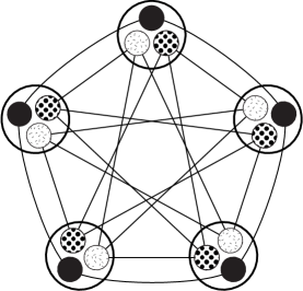
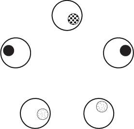
Figure 1: Example $(3,2)$-CSP instance with five variables and twenty constraints (left), and a solution of the instance (right).

      

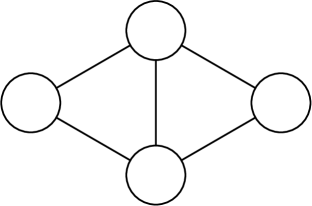
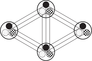
Figure 2: Example $3$-coloring instance (left) and translation into a $(3,2)$-CSP instance (right).

For instance, $3$-satisfiability can easily be expressed in this form. Each variable of the satisfiability problem may be colored (assigned the value) either true ($T$) or false ($F$). For each clause like $(x_{1}\vee x_{2}\vee\neg{x}_{3})$, we make a constraint $((v_{1},F),(v_{2},F),(v_{3},T))$. Such a constraint is satisfied if and only if at least one of the corresponding clause’s terms is true.

In the $(a,b)$-CSP problem, we restrict our attention to instances in which each variable has at most $a$ possible colors and each constraint involves at most $b$ variables. The CSP instance constructed above from a $3$-SAT instance is then a $(2,3)$-CSP instance, and in fact $3$-SAT is easily seen to be equivalent to $(2,3)$-CSP.

In this paper, we will concentrate our attention instead on $(3,2)$-CSP and $(4,2)$-CSP. We can represent a $(d,2)$-CSP instance graphically, by interpreting each variable as a vertex containing up to $d$ possible colors, and by drawing edges connecting incompatible pairs of vertex colors (Figure 1). Note that this graphical structure is not actually a graph, as the edges connect colors within a vertex rather than the vertices themselves. However, graph $3$-colorability and graph $3$-list-colorability can be translated directly to a form of $(3,2)$-CSP: we keep the original vertices of the graph and their possible colors, and add up to three constraints for each edge of the graph to enforce the condition that the edge’s endpoints have different colors (Figure 2).

Of course, since these problems are all NP-complete, the theory of NP-completeness provides translations from one problem to the other, but the translations above are size-preserving and very simple. Our graph coloring techniques include more complicated translations in which the input graph is partially colored before treating the remaining graph as an CSP instance, leading to improved time bounds over our pure CSP algorithm.

3 Constraint Satisfaction Algorithm

We now outline our $(4,2)$-CSP algorithm. A $(4,2)$-CSP instance can be transformed into a $(3,2)$-CSP instance by expanding its four-color variables to two three-color variables (Figure 3), so a natural definition of the “size” of a $(4,2)$-CSP instance is $n=n_{3}+2n_{4}$, where $n_{i}$ denotes the number of $i$-color variables. However, we instead define the size as $n=n_{3}+(2-\epsilon)n_{4}$, where $\epsilon$ is a constant to be determined later. The size of a $(3,2)$-CSP instance remains equal to its number of variables, so any bound on the running time of our algorithm in terms of $n$ applies directly to $(3,2)$-CSP.

Our basic idea is to find a set of local configurations that must occur within any $(4,2)$-CSP instance $I$. For each configuration we describe a set of smaller instances $I_{i}$ of size $|I|-r_{i}$ such that $I$ is solvable if and only if at least one of the instances $I_{i}$ is solvable. If one particular configuration occurred at each step of the algorithm, this would lead to a recurrence of the form

$$T(n)=\sum T(n-r_{i})+\hbox{poly}(n)=O(\lambda(r_{1},r_{2},\ldots)^{n})$$

for the runtime of our algorithm, where $\lambda(r_{1},r_{2},\ldots)$ is the largest zero of the function $f(x)=1-\sum x^{-r_{i}}$. We call this value $\lambda(r_{1},r_{2},\ldots)$ the work factor of the given local configuration. The overall time bound will be $\lambda^{n}$ where $\lambda$ is the largest work factor among the configurations we identify.

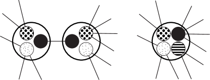
Figure 3: Isolated constraint between two three-color variables (left) is equivalent to a single four-color variable (right).

We first consider local configurations in which some (variable,color) pair $(v,R)$ is involved in only a single constraint $((v,R),(w,R))$. If this is also the only constraint involving $(w,R)$, and both $v$ and $w$ have three colors, they can be replaced by a single four-color variable (Figure 3); any other singly-constrained color leads to a problem reduction with work factor $\lambda(2-\epsilon,$3$-\epsilon)$.

We next find colors with multiple constraints to different colors of the same variable, and show that such a case has work factor $\lambda(2-\epsilon,$3$-2\epsilon)$. The next case we consider involves colors constrained by four or more neighboring variables, or four-color variables with a color constrained by three variables. In these cases, choosing to use or not use the highly-constrained color gives work factor $\lambda(1-\epsilon,5-4\epsilon)$. Instances in which none of the above cases applies have a special form: each (variable,color) pair has exactly two or three constraints, which must involve distinct variables.

Our next sequence of cases concerns adjacency between (variable,color) pairs with two constraints and pairs with three constraints. We show that, if $(v,R)$ has three constraints, one of which connects it to a variable with four color choices, then the instance can be replaced by smaller instances with work factor at most $\lambda($3$-\epsilon,4-\epsilon,4-\epsilon)$. If this case does not apply, and a three-constraint pair $(v,R)$ is adjacent to a (variable,color) pair with two constraints, then we have additional cases with work factor at most $\mathop{\rm max}\{\lambda(1+\epsilon,4),\lambda(3,4-\epsilon,4)\}$. If none of these cases applies to an instance, then each color choice in the instance must have either two or three constraints, and each neighbor of that choice must have the same number of constraints.

We now consider the remaining (variable,color) pairs that have three constraints each. Define a three-component to be a subset of such pairs such that any pair in the subset is connected to any other by a path of constraints. We distinguish two such types of components: a small three-component is one that involves only four distinct variables, while a large three-component involves five or more variables. A small three-component is good if it involves only four (variable,color) pairs. We show that an instance containing a small three-component that is not good can be replaced by smaller instances with work factor at most $\lambda(4,4,4)$, and that an instance containing a large three-component can be replaced by smaller instances with work factor at most $\lambda(4,4,5,5)$. As a consequence, we can assume all remaining three-components are good.

Finally, we define a two-component to be a subset of (variable,color) pairs such that each has two constraints, and any pair in the subset is connected to any other by a path of constraints. Our analysis of two-components is essentially the same as in [2], and shows that unless a two-component forms a triangle, the instance can be replaced by smaller instances with work factor at most $\lambda(3,3,5)$.

Suppose we have a $(4,2)$-CSP instance to which none of the preceding reduction cases applies. Then, every constraint must be part of a good three-component or a triangular two-component. As we now show, this simple structure enables us to solve the remaining problem quickly.

Lemma 1

If we are given a $(4,2)$-CSP instance in which every constraint must be part of a good three-component or a small two-component, then we can solve it or determine that it is not solvable in polynomial time.

Proof: We form a bipartite graph, in which the vertices correspond to the variables and components of the instance. We connect a variable to a component by an edge if there is a (variable,color) pair using that variable and belonging to that component. The instance is solvable iff this graph has a matching covering all variables.

This completes the analysis needed for our result.

Theorem 1

We can solve any $(3,2)$-CSP instance in time $O(\lambda(4,4,5,5)^{n})\approx O(1.36443^{n})$.

Proof: We employ a backtracking (depth first) search in a state space consisting of $(3,2)$-CSP instances. At each step we examine the current state, match it to one of the cases above, and recursively search each smaller instance. If we reach an instance in which Lemma 1 applies, we perform a matching algorithm and either stop with a solution or backtrack to the most recent branching point of the search and continue with the next alternative.

A bound of $\lambda^{n}$ on the number of recursive calls in this search algorithm, where $\lambda$ is the maximum work factor occurring in our reduction lemmas, can be proven by induction on the size of an instance. To determine the maximum work factor, we need to set the parameter $\epsilon$. We used Mathematica to optimize $\epsilon$ numerically, and found that for $\epsilon\approx 0.095543$ the work factor is $\approx 1.36443\approx\lambda(4,4,5,5)$. For $\epsilon$ near this value, the largest work factors involving $\epsilon$ are $\lambda($3$-\epsilon,4-\epsilon,4-\epsilon)$, and $\lambda(1+\epsilon,4)$; the remaining work factors are below 1.36. The true optimum value of $\epsilon$ is thus the one for which $\lambda($3$-\epsilon,4-\epsilon,4-\epsilon)=\lambda(1+\epsilon,4)$.

As we now show, for this optimum $\epsilon$, $\lambda($3$-\epsilon,4-\epsilon,4-\epsilon)=\lambda(1+\epsilon,4)=\lambda(4,4,5,5)$, which also arises as a work factor in another case. Consider subdividing an instance of size $n$ into one of size $n-(1+\epsilon)$ and another of size $n-4$, and then further subdividing the first instance into subinstances of size $n-(1+\epsilon)-($3$-\epsilon)$, $n-(1+\epsilon)-(4-\epsilon)$, and $n-(1+\epsilon)-(4-\epsilon)$. This four-way subdivision has work factor $\lambda(4,4,5,5)$, and combines subdivisions of type $\lambda(1+\epsilon,4)$ and $\lambda($3$-\epsilon,4-\epsilon,4-\epsilon)$, so these three work factors must be equal.

We use the quantity $\lambda(4,4,5,5)$ frequently in the remainder of the paper, so we use $\Lambda$ to denote this value. Theorem 1 immediately gives algorithms for some more well known problems, some of which we improve later. Of these, the least familiar is likely to be list $k$-coloring: given at each vertex of a graph a list of $k$ colors chosen from some larger set, find a coloring of the whole graph in which each vertex color is chosen from the corresponding list [11].

Corollary 1

We can solve the $3$-coloring and $3$-list coloring problems in time $O(\Lambda^{n})$, the $3$-edge-coloring problem in time $O(\Lambda^{m})$, and the $3$-SAT problem in time $O(\Lambda^{t})$,

Corollary 2

There is a randomized algorithm which finds the solution to any solvable $(d,2)$-CSP instance (with $d>3$) in expected time $O((0.4518d)^{n})$.

Proof: Randomly choose a subset of four values for each variable and apply our algorithm to the resulting $(4,2)$-CSP problem. Repeat with a new random choice until finding a solvable $(4,2)$-CSP instance. The random restriction of a variable has probability $4/d$ of preserving solvability so the expected number of trials is $(d/4)^{n}$. Each trial takes time $O(\Lambda^{(2-\epsilon)n})\approx O(1.8072^{n})$. The total expected time is therefore $O((d/4)^{n}1.8072^{n})$.

4 Vertex Coloring

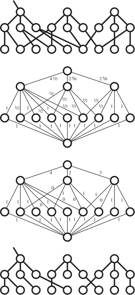
Figure 4: Use of maximum flow to find a good height-two forest. Top: forest of $K_{1,3}$ subgraphs and adjacent vertices. The left subgraph is adjacent to the maximal bushy forest; the other two subgraphs are not. Top middle: flow graph and fractional flow formed by spreading flow equally from each of the bottom vertices. The edge capacities are all one, except for the top three which are respectively 5, 3, and 3. Bottom middle: maximum integer flow for the same flow graph. Bottom: height-two forest corresponding to the given integer flow.

Simply by translating a $3$-coloring problem into a $(3,2)$-CSP instance, as described above, we can test $3$-colorability in time $O(\Lambda^{n})$. We reduce this further (as in [2]) by finding a small set of vertices $S\subset V(G)$ with a large set $N$ of neighbors, and choosing one of the $3^{|S|}$ colorings for all vertices in $S$. For each such coloring, we translate the remaining problem to a $(3,2)$-CSP instance. The vertices in $S$ are already colored and need not be included in the $(3,2)$-CSP instance, and the vertices in $N$ can also be eliminated, so the overall time is $O(3^{|S|}\Lambda^{|V(G)-S-N|})$. By choosing $S$ appropriately we can make this quantity smaller than $O(\Lambda^{n})$.

We begin by showing a cycle of degree-three vertices allows us to reduce a $3$-coloring instance to smaller instances with work factor $\lambda(5,6,7,8)\approx 1.2433$, and that a tree of eight or more such vertices leads to work factor $\lambda(2,5,6)\approx 1.3247$. Therefore, we can assume that the degree-three vertices form trees of at most seven vertices, and that the graph contains many higher degree vertices.

We define a bushy forest to be an unrooted forest within a given instance graph, such that each internal node has degree four or more. Because each tree of $k$ degree-three vertices must have at least $9k/7$ outgoing edges, we can show that the number of vertices excluded from a maximal bushy forest is at most $20r/3$, where $r$ is its number of leaves.

All internal nodes of the maximal bushy forest $F$ will be included in $S$, but we also wish to include some of the remaining graph vertices. To do this, we form these vertices into trees of height two, with at most five grandchildren. Further, in a tree with four or more grandchildren, at least one node must have degree four or more in $G$. This forest of height-two trees can be found by the following flow-based technique (Figure 4): first, find a set of disjoint $K_{1,3}$ subgraphs in $G\setminus F$, maximal under operations that remove one such subgraph and form two or more from the remaining vertices. Assign grandchildren to these height-one trees, from the remaining vertices nonadjacent to $F$, with fractional weights spread evenly among the trees each child can be assigned to. This fractional assignment can be shown to have the bounds we want on the total assigned weight of grandchildren per tree, but does not form a disjoint set of trees. However, we can represent the possible assignments of grandchildren to trees using a flow graph, and use the fact that every flow problem has an optimal integer solution, to find a non-fractional assignment of grandchildren to trees with the same bounds. We will add to $S$ certain tree roots or their children, depending on the shape of each height-two tree.

Theorem 2

We can solve the $3$-coloring problem in time $O((2^{3/49}3^{4/49}\Lambda^{24/49})^{n})\approx 1.3289^{n}$.

Proof: As described, we find a maximal bushy forest $F$, then cover the remaining vertices by height-two trees. We choose colors for each internal vertex in $F$, and for certain vertices in the height-two trees. Vertices adjacent to these colored vertices are restricted to two colors, while the remaining vertices form a $(3,2)$-CSP instance and can be colored using our general $(3,2)$-CSP algorithm.

Let $p$ denote the number of vertices that are roots in $F$; $q$ denote the number of non-root internal vertices; $r$ denote the number of leaves of $F$; $s$ denote the number of vertices adjacent to leaves of $F$; and $t$ denote the number of remaining vertices, which must all be degree-three vertices in the height-two forest. We show that, if we assign cost $\Lambda$ to each vertex adjacent to a leaf of $F$, then the cost of coloring each height-two tree, averaged over its remaining vertices, is at most $(3\Lambda^{3})^{1/7}$ per vertex. Therefore, the total time for the algorithm is at most $3^{p}2^{q}\Lambda^{s}(3\Lambda^{3})^{t/7}$.

This bound is subject to the constraints $p,q,r,s,t\geq 0$, $p+q+r+s+t=n$, $4p+2q\leq r$, $2r\geq s$, and $20r/3\geq s+t$. The worst case occurs when $s+t=20r/3$, $s=2r$, $t=14r/3$, $4p+2q=r$, $p=0$, and $r=2q$, giving the stated bound.

5 Edge Coloring

We now describe an algorithm for finding edge colorings of undirected graphs, using at most three colors, if such colorings exist. We can assume without loss of generality that the graph has vertex degree at most three. Then $m\leq 3n/2$, so by applying our vertex coloring algorithm to the line graph of $G$ we could achieve time bound $1.3289^{3n/2}\approx 1.5319^{n}$. Just as we improved our vertex coloring algorithm by performing some reductions in the vertex coloring model before treating the problem as a $(3,2)$-CSP instance, we improve this edge coloring bound by performing some reductions in the edge coloring model before treating the problem as a vertex coloring instance.

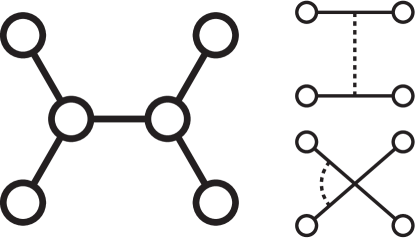
Figure 5: Replacement of five edges (left) by two constrained edges (right).

The main idea is to solve a problem intermediate in generality between $3$-edge-coloring and $3$-vertex-coloring: $3$-edge-coloring with some added constraints that certain pairs of edges should not be the same color.

Lemma 2

Suppose a constrained $3$-edge-coloring instance contains an unconstrained edge connecting two degree-three vertices. Then the instance can be replaced by two smaller instances with three fewer edges and two fewer vertices each.

This reduction operation is depicted in Figure 5.

We let $m_{3}$ denote the number of edges with three neighbors in an unconstrained $3$-edge-coloring instance, and $m_{4}$ denote the number of edges with four neighbors. Edges with fewer neighbors can be removed at no cost, so we can assume without loss of generality that $m=m_{3}+m_{4}$. By using a maximum matching algorithm, we can find a set of $m_{4}/3$ edges such that Lemma 2 can be applied independently to each edge.

Theorem 3

We can $3$-edge-color any $3$-edge-colorable graph, in time $O(2^{n/2})$.

Proof: We apply Lemma 2 $m_{4}/3$ times, resulting in a set of $2^{m_{4}/3}$ constrained $3$-edge-coloring problems each having only $m_{3}$ edges. We then treat these remaining problems as $3$-vertex-coloring problems on the corresponding line graphs, augmented by additional edges representing the constraints added by Lemma 2. The time for this algorithm is thus at most $O(1.3289^{m_{3}}2^{m_{4}/3})$. This is maximized when $m_{4}=3n/2$ and $m_{3}=0$.

References

- [1] N. Alon and N. Kahale. A spectral technique for coloring random -colorable graphs. SIAM J. Comput. 26(6):1733–1748, 1997, http://www.research.att.com/~kahale/papers/jour.ps.
- [2] R. Beigel and D. Eppstein. 3-coloring in time : a no-MIS algorithm. Proc. 36th Symp. Foundations of Computer Science, pp. 444–453. Inst. of Electrical & Electronics Engineers, October 1995, ftp://ftp.eccc.uni-trier.de/pub/eccc/reports/1995/TR95-033/index.html.
- [3] R. Beigel and D. Eppstein. 3-coloring in time . ACM Computing Research Repository, June 2000. cs.DS/0006046.
- [4] A. Blum and D. Karger. An -coloring algorithm for -colorable graphs. Inf. Proc. Lett. 61(1):49–53, 1997, http://www.cs.cmu.edu/~avrim/Papers/color_new.ps.gz.
- [5] E. Dantsin. Two systems for proving tautologies, based on the split method. J. Sov. Math. 22:1293–1305, 1983. Original Russian article appeared in 1981.
- [6] E. Dantsin and E. A. Hirsch. Algorithms for -SAT based on covering codes. Preprint 1/2000, Steklov Inst. of Mathematics, 2000, ftp://ftp.pdmi.ras.ru/pub/publicat/preprint/2000/01-00.ps.gz.
- [7] M. Davis and H. Putnam. A computing procedure for quantification theory. J. ACM 7(3):201–215, 1960.
- [8] T. Feder and R. Motwani. Worst-case time bounds for coloring and satisfiability problems. Manuscript, September 1998.
- [9] J. Gramm, E. A. Hirsch, R. Niedermeier, and P. Rossmanith. Better worst-case upper bounds for MAX-2-SAT. 3rd Worksh. on the Satisfiability Problem, 2000, http://ssor.twi.tudelft.nl/~warners/SAT2000abstr/hirsch.html.
- [10] E. A. Hirsch. Two new upper bounds for SAT. Proc. 9th ACM-SIAM Symp. Discrete Algorithms, pp. 521–530, 1998, http://logic.pdmi.ras.ru/~hirsch/abstracts/soda98.html.
- [11] T. R. Jensen and B. Toft. Graph Coloring Problems. Ser. Discrete Mathematics and Optimization. John Wiley & Sons, Inc., New York, 1995.
- [12] O. Kullmann. New methods for 3-SAT decision and worst-case analysis. Theor. Comp. Sci. 223(1–2):1–72, July 1999, http://www.cs.toronto.edu/~kullmann/3neu.ps.
- [13] O. Kullmann and H. Luckhardt. Various upper bounds on the complexity of algorithms for deciding propositional tautologies. Manuscript available from kullmann@mi.informatik.uni-frankfurt.de, 1994.
- [14] V. Kumar. Algorithms for constraint satisfaction problems: a survey. AI Magazine 13(1):32–44, 1992, http://citeseer.nj.nec.com/kumar92algorithms.html.
- [15] E. L. Lawler. A note on the complexity of the chromatic number problem. Inf. Proc. Lett. 5(3):66–67, August 1976.
- [16] H. Luckhardt. Obere Komplexitätsschranken für TAUT-Entscheidungen. Proc. Frege Conf., Schwerin, pp. 331–337. Akademie-Verlag, 1984.
- [17] B. Monien and E. Speckenmeyer. Solving satisfiability in less than steps. Discrete Appl. Math. 10(3):287–295, March 1985.
- [18] R. Paturi, P. Pudlák, M. E. Saks, and F. Zane. An improved exponential-time algorithm for -SAT. Proc. 39th Symp. Foundations of Computer Science, pp. 628–637. IEEE, 1998, http://www.math.cas.cz/~pudlak/ppsz.ps.
- [19] A. D. Petford and D. J. A. Welsh. A randomised -colouring algorithm. Discrete Math. 74(1–2):253–261, 1989.
- [20] R. Rodošek. A new approach on solving 3-satisfiability. Proc. 3rd Int. Conf. Artificial Intelligence and Symbolic Mathematical Computation, pp. 197–212. Springer-Verlag, Lecture Notes in Computer Science 1138, 1996, http://www-icparc.doc.ic.ac.uk/papers/a_new_approach_on_solving_3-satis%fiabili.ps.
- [21] I. Schiermeyer. Solving 3-satisfiability in less than steps. Proc. 6th Worksh. Computer Science Logic, pp. 379–394. Springer-Verlag, Lecture Notes in Comp. Sci. 702, 1993.
- [22] I. Schiermeyer. Deciding 3-colourability in less than steps. Proc. 19th Int. Worksh. Graph-Theoretic Concepts in Computer Science, pp. 177–182. Springer-Verlag, Lecture Notes in Comp. Sci. 790, 1994.
- [23] U. Schöning. A probabilistic algorithm for k-SAT and constraint satisfaction problems. Proc. 40th IEEE Symp. Foundations of Computer Science, pp. 410–414, October 1999.
- [24] B. Selman. Satisfiability testing: theory and practice. DIMACS Worksh. Faster Exact Solutions for NP-Hard Problems, February 2000.
- [25] R. D. Vlasie. Systematic generation of very hard cases for graph 3-colorability . Proc. 7th IEEE Int. Conf. Tools with Artificial Intelligence, pp. 114–119, 1995, http://www.essi.fr/~vlasier/PS/3paths.ps.