Examples, Counterexamples, and
Enumeration Results for
Foldings and Unfoldings
between Polygons and Polytopes

Abstract

We investigate how to make the surface of a convex polyhedron (a polytope) by folding up a polygon and gluing its perimeter shut, and the reverse process of cutting open a polytope and unfolding it to a polygon. We explore basic enumeration questions in both directions: Given a polygon, how many foldings are there? Given a polytope, how many unfoldings are there to simple polygons? Throughout we give special attention to convex polygons, and to regular polygons. We show that every convex polygon folds to an infinite number of distinct polytopes, but that their number of combinatorially distinct gluings is polynomial. There are, however, simple polygons with an exponential number of distinct gluings.

In the reverse direction, we show that there are polytopes with an exponential number of distinct cuttings that lead to simple unfoldings. We establish necessary conditions for a polytope to have convex unfoldings, implying, for example, that among the Platonic solids, only the tetrahedron has a convex unfolding. We provide an inventory of the polytopes that may unfold to regular polygons, showing that, for $n>6$, there is essentially only one class of such polytopes.

1 Introduction

We explore the process of folding a simple polygon by gluing its perimeter shut to form a convex polyhedron, and its reverse, cutting a convex polyhedron open and flattening its surface to a simple polygon. We restrict attention to convex polyhedra (henceforth, polytopes), and to simple (i.e., nonself-intersecting, nonoverlapping) polygons (henceforth just polygons). The restriction to nonoverlapping polygons is natural, as this is important to the manufacturing applications [O’R00]. The restriction to convex polyhedra is made primarily to reduce the scope of the problem. See  [BDD⁺98] and [BDEK99] for a start on unfolding nonconvex polyhedra.

Much recent work on unfolding revolves around an open problem that seems to have been first mentioned in print in [She75] but is probably much older: Can every polytope be cut along edges and unfolded flat to a (simple) polygon? Cutting along edges leads to edge unfoldings; we will not follow this restriction here. Thus our work is only indirectly related to this edge-unfolding question.

In some sense this report is a continuation of the investigation started in [LO96], which detailed an $O(n^{2})$ algorithm for deciding when a polygon may be folded to a polytope, with the restriction that each edge of the polyon perimeter glues to another complete edge: edge-to-edge gluing. But here we do not following this restriction, permitting arbitrary perimeter gluings. Moreover, we do not consider algorithmic questions. Rather we concentrate on enumerating the number of foldings and unfoldings between polygons and polytopes. We pay special attention to convex polygons; following Shephard [She75], we call an unfolding of a polytope that produces a convex polygon a convex unfolding. Within the class of polytopes, we sometimes use the five regular polytopes as examples; within the class of convex polygons, we additionally focus on regular polygons.

The basic questions we ask are:

1. How many combinatorially different foldings of a polygon lead to a polytope?

2. How many geometrically different polytopes may be folded from one polygon?

3. How many combinatorially different cuttings of a polytope lead to polygon unfoldings?

4. How many geometrically different polygons may be unfolded from one polytope?

Our answers to these four questions are crudely summarized in Table 1, whose four rows correspond to the four questions above, and whose columns are for general, convex, and regular polygons. We will not explain the entries in the table here, but only remark that the increased constraints provided by convex and regular polygons reduces the number of possibilities.

		General	Convex	Regular
			Polygons	Polygons
Foldings	gluing trees	$2^{\Omega(n)}$, $O(n^{2{\lambda}-2})$	$O(n^{3})$	$O(1)$
	polytopes	$\infty$	$\infty$	$2$ classes
Unfoldings	cut trees	$2^{\Omega(n)}$, $2^{O(n^{2})}$	?	$O(1)$
	polygons	$\infty$	$0$, $\infty$	$O(1)$

Table 1: Summary of Results. $n$ is the number of polygon vertices or polytope vertices; ${\lambda}$ is the number of leaves of the gluing tree; the symbol $\infty$ represents nondenumerably infinite, i.e., a continuum.

A key tool in our work is a powerful theorem of Aleksandrov, which we describe and immediately apply in Section 2. We then define the two main combinatorial objects we study, cut trees and gluing trees, and make clear exactly how we count them. We then explore constraints on convex unfoldings in Section 4 before proceeding to the general enumeration bounds in Table 1 in Sections 5-8. A final section (9) concentrates on regular polygons

2 Aleksandrov’s Theorem

Aleksandrov proved a far-reaching generalization of Cauchy’s rigidity theorem in [Ale58] that gives simple conditions for any folding to a polytope. Let $P$ be a polygon and ${\partial P}$ its boundary. A gluing maps ${\partial P}$ to ${\partial P}$ in a length-preserving manner, as follows. ${\partial P}$ is partitioned by a finite number of distinct points into a collection of open intervals whose closure covers ${\partial P}$. Each interval is mapped one-to-one (i.e., glued) to another interval of equal length. Corresponding endpoints of glued intervals are glued together (i.e., identified). Finally, gluing is considered transitive: if points $a$ and $b$ glue to point $c$, then $a$ glues to $b$. Aleksandrov proved that any gluing that satisfies these two conditions corresponds to a unique polytope:

1. No more than $2\pi$ total face angle is glued together at any point; and

2. The complex resulting from the gluing is homeomorphic to a sphere. (This condition is satisfied if, when ${\partial P}$ is viewed as a topological circle, and the interval gluings as chords of the circle, then no pair of chords cross in the ${\partial P}$-circle.)

Aleksandrov calls any complex (not necessarily a single polygon) that satisfies these properties a net [Ale58]. We call a gluing that satisfies these conditions an Aleksandrov gluing.

Although an Aleksandrov gluing of a polygon forms a unique polytope, it is an open problem to compute the three-dimensional structure of the polytope [O’R00]. Note that there is no specification of the fold (or “crease”) lines; and yet they are uniquely determined. Henceforth we will say a polygon folds to a polytope whenever it has an Aleksandrov gluing.

We should mention two features of Aleksandrov’s theorem. First, the polytope whose existence is guaranteed may be flat, that is, a doubly-covered convex polygon. We use the term “polytope” to include flat polyhedra. Second, condition (2) specifies a face angle $\leq 2\pi$. The case of equality with $2\pi$ leads to a point on the polytope at which there is no curvature, i.e., a nonvertex. We make explicit what counts as a vertex below.

Polygon/Polytope Notation.

We will use $P$ throughout the paper for a polygon, and $Q$ for a polytope. Their boundaries are ${\partial P}$ and ${\partial Q}$ respectively. The curvature ${\gamma}(x)$ of a point $x\in{\partial Q}$ is $2\pi$ minus the sum of the face angles incident to $x$. This “angle deficit” corresponds to the notion of Gaussian curvature. We define vertices of polygons and polytopes to be essential in the sense that the boundary is not flat there: the interior angle at a polygon vertex is different from $\pi$, and the curvature at a polytope vertex is different from $0$. Because of these definitions, there is no direct correspondence between the vertices of a polytope $Q$ and the vertices of a polygon $P$ unfolding of $Q$: a vertex of $Q$ may or may not unfold to a vertex of $P$; and a vertex of $P$ may or may not fold to a vertex of $Q$ (see Section 3.3). At the risk of confusion, we will use the terms “vertex” and “edge” for both polygons and polytopes, but reserve “node” and “arc” for graphs. We will use $n$ for the number of vertices of $P$ or $Q$, letting the context determine which.

We will also freely employ two types of paths on the surface of a polytope: geodesics, which unfold (or “develop”) to straight lines, and shortest paths, geodesics which are in addition shortest paths between their endpoints. See, e.g., [AAOS97] for details and basic properties.

2.1 Perimeter Halving

As a straightforward application of Aleksandrov’s theorem, we prove that every convex polygon folds to a polytope. We will see in Section 4.2 that the converse does not hold.

For two points $x,y\in{\partial P}$, define $(x,y)$ be the open interval of ${\partial P}$ counterclockwise from $x$ to $y$, and let $|x,y|$ be its length. Define a perimeter-halving gluing as one which glues $(x,y)$ to $(y,x)$.

Lemma 2.1

Every convex polygon folds to a polytope via perimeter halving.

Proof: Let the perimeter of a convex polygon $P$ be $L$. Let $x\in{\partial P}$ be an arbitrary point on the boundary of $P$, and let $y\in{\partial P}$ be the midpoint of perimeter around ${\partial P}$ measured from $x$, i.e., $y$ is the unique point satisfying $|x,y|=|y,x|=L/2$. See Fig. 1 for an example.

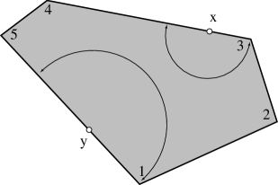
Figure 1: A perimeter-halving fold of a pentagon. The gluing mappings of vertices $v_{1}$ and $v_{3}$ are shown.

Now glue $(x,y($ to $(y,x)$ in the natural way, mapping each point $z$ with $|x,z|=d$ to the point $z^{\prime}$ the same distance from $x$ in the other direction: $|z^{\prime},x|=d$. We claim this is an Aleksandrov gluing. It is a gluing by construction. Because $P$ is convex, each point along the gluing path has $\leq 2\pi$ angle incident to it: the gluing of two nonvertex points results in exactly $2\pi$, and if either point is a vertex, the total angle is strictly less than $2\pi$. The resulting surface is clearly homeomorphic to a sphere. By Aleksandrov’s theorem, this gluing corresponds to a unique polytope $Q_{x}$. $\Box$

In an Aleksandrov gluing of a polygon, a point in the interior of a polygon edge that glues only to itself, i.e., where a crease folds the edge in two, is called a fold point. A fold point corresponds to a leaf of the gluing tree, and becomes a vertex of the polytope with curvature $\pi$. Points $x$ and $y$ in the above proof are fold points. In Theorem 6.2 we will show that different choices of $x$ result in distinct polytopes $Q_{x}$, leading to the conclusion that every convex polygon folds to an infinite number of polytopes.

3 Cut Trees and Gluing Trees

The four main objects we study are polygons, polytopes, cut trees, and gluing trees. It will be useful in spots to distinguish between a geometric tree ${\cal T}$ composed of a union of line segments, and the more familiar combinatorial tree $T$ of nodes and arcs. A geometric cut tree ${\cal T}_{C}$ for a polytope $Q$ is a tree drawn on ${\partial Q}$, with each arc a polygonal path, which leads to a polygon unfolding when the surface is cut along ${\cal T}$, i.e., flattening $Q\setminus{\cal T}$ to a plane. A geometric gluing tree ${\cal T}_{G}$ specifies how ${\partial P}$ is glued to itself to fold to a polytope. There is clearly a close correspondence between ${\cal T}_{C}$ and ${\cal T}_{G}$, which are in some sense the same object, one viewed from the perspective of unfolding, one from the perspective of folding. It will nevertheless be useful to retain a distinction between them, and especially their combinatorial counterparts, which we define below after stating some basic properties.

3.1 Cut Trees

Lemma 3.1

If a polygon $P$ folds to a polytope $Q$, ${\partial P}$ maps to a tree ${\cal T}_{C}\subset{\partial Q}$, the geometric cut tree, with the following properties:

1. ${\cal T}_{C}$ is a tree.

2. ${\cal T}_{C}$ spans the vertices of $Q$.

3. Every leaf of ${\cal T}_{C}$ is at a vertex of $Q$.

4. A point of ${\cal T}_{C}$ of degree $d$ (i.e., one with $d$ incident segments) corresponds to exactly $d$ points of ${\partial P}$. Thus a leaf corresponds to a unique point of ${\partial P}$.

5. Each arc of $T_{C}$ is a polygonal path on $Q$.

Proof:

1. If ${\cal T}_{C}$ contained a cycle, then it would unfold to disconnected pieces, contradicting the assumption that $Q$ is folded from a single polygon $P$. Thus ${\cal T}_{C}$ is a forest. But because ${\cal T}_{C}$ is constructed by gluing the connected path ${\partial P}$ to itself, it must be connected. So ${\cal T}_{C}$ is a tree.

2. If a vertex $v$ of $Q$ is not touched by ${\cal T}_{C}$, then, because $Q$ is not flat at $v$, $P$ is not planar, a contradiction to the assumption that $P$ is a polygon.

3. Suppose a leaf $x$ of ${\cal T}_{C}$ is interior to a face or edge of $Q$. Then it is surrounded by $2\pi$ face angle on $Q$, and so unfolds to a point $x$ of $P$ similarly surrounded. But by assumption, $x$ is on the boundary of a simple polygon $P$, a contradiction.

4. Gluing exactly two distinct points of $x,y\in{\partial P}$ together implies that neighborhoods of $x$ and $y$ are glued, which leads to the interior of an arc of the cut tree, i.e., a degree-$2$ point of ${\cal T}_{C}$. Note that either or both of these points might be vertices of $P$. In general, if $p\in{\cal T}_{C}$ has $d$ incident cut segments, $p$ unfolds to $d$ distinct points of ${\partial P}$.

5. If an arc of ${\cal T}_{C}$ is not a polygonal path, then neither side unfolds to a polygonal path, contradicting the assumption that $P$ is a polygon.

$\Box$

When counting cut trees, we will rely on their combinatorial structure. There are several natural definitions of this structure, which are useful in different circumstances. We first discuss some of the options.

1. Make every segment of ${\cal T}_{C}$ an arc of $T_{C}$. Although this is very natural, it means there are an infinite number of different cut trees for any polytope, for the path between any two polytope vertices could be an arbitrarily complicated polygonal path, leading to different combinatorial trees.

2. Make every point where a path of ${\cal T}_{C}$ crosses an edge of the polytope a node of $T_{C}$. This again leads to trivially infinite numbers of cut trees when a path of ${\cal T}_{C}$ zigzags back and forth over an edge of $Q$.

3. Exclude this possibility by forcing the paths between polytope vertices to be geodesics, and again make polytope edge crossings nodes of $T_{C}$. This excludes many interesting cut trees—all those where a polygon vertex is glued to a point with angle sum $2\pi$.

4. Make every maximal path of ${\cal T}_{C}$ consisting only of degree-$2$ points a single arc of $T_{C}$. This has the undesirable effect of having polytope vertices in the interior of such a path disappear from $T_{C}$.

Threading between these possibilities, we define the combinatorial cut tree $T_{C}$ corresponding to a geometric cut tree ${\cal T}_{C}$ as the labeled graph with a node (not necessarily labeled) for each point of ${\cal T}_{C}$ with degree not equal to $2$, and a labeled node for each point of ${\cal T}_{C}$ that corresponds to a vertex of $Q$ (labeled by the vertex label); arcs are determined by the polygonal paths of ${\cal T}_{C}$ connecting these nodes. An example is shown in Fig. 2. Note that not every node of the tree is labeled, but every polytope vertex label is used at some node. All degree-$2$ nodes are labeled.

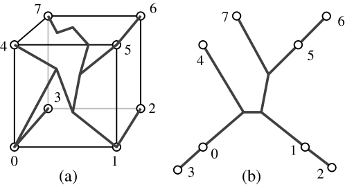
Figure 2: (a) Geometric cut tree ${\cal T}_{C}$ on the surface of a cube; (b) The corresponding combinatorial cut tree $T_{C}$.

Although this definition avoids some of the listed pitfalls, it does have the undesirable consequence of counting different geodesics on ${\partial Q}$ between two polytope vertices as the same arc of $T_{C}$. Thus the two unfoldings shown in Fig. 5 (below) have the same combinatorial cut tree under our definition, even though the geodesic in (c) spirals twice around compared to once around in (a).

3.2 Gluing Trees

Let a convex polygon $P$ have vertices $v_{1},\ldots,v_{n}$, labeled counterclockwise, and edge $e_{i}$, $i=1,\ldots,n$ the open segment of ${\partial P}$ after $v_{i}$. There is less need to discuss the geometric gluing tree, so we concentrate on the combinatorial gluing tree $T_{G}$. $T_{G}$ is a tree representing the identification of ${\partial P}$ with itself. Any point of ${\partial P}$ that is identified with more or less than one other distinct point of ${\partial P}$ becomes a node of $T_{G}$, as well as any point to which a vertex is glued. (Note that this means there may be nodes of degree $2$.) So every vertex of $P$ maps to a node of $T_{G}$; each node is labeled with the set of all the elements (vertices or edges) that are glued together there. A leaf that is a fold point is labeled by the edge label only. Every nonleaf node has at least one vertex label, and at most one edge label. A simple example is shown in Fig. 3. Here the central node of $T_{G}$ is assigned the label $\{v_{1},v_{3},e_{3}\}$.

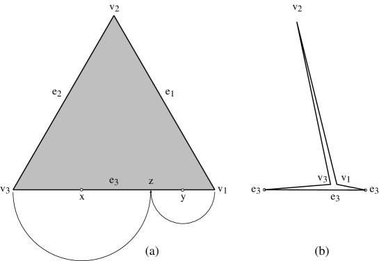
Figure 3: (a) A gluing of an equilateral triangle $P$: $v_{1}$ and $v_{3}$ are glued to point $z$; (b) the corresponding gluing tree $T_{G}$ [folding up]. Points $x$ and $y$ become fold points of the resulting tetrahedron.

A more complicated example is shown in Fig. 4. The polygon shown folds (amazingly!) to a tetrahedron by creasing as illustrated in (a). All four tetrahedron vertices are fold points. The corresponding gluing tree is shown in (b) of the figure. The two interior nodes of $T_{G}$ have labels $\{v_{1},v_{6},e_{1}\}$ and $\{v_{2},v_{5},e_{5}\}$.

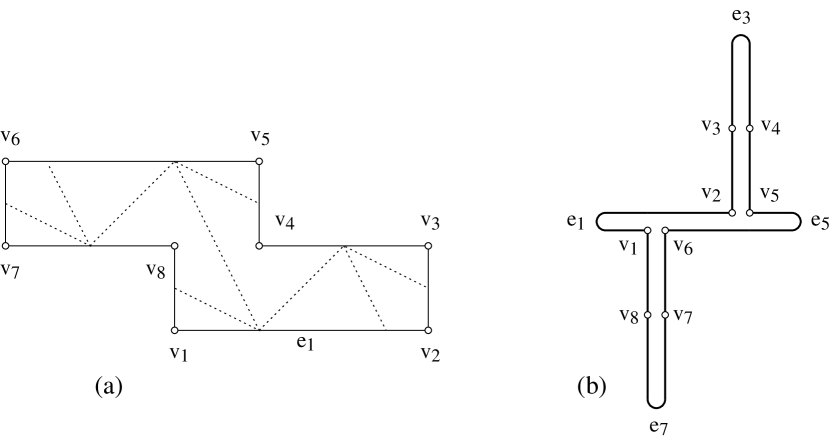
Figure 4: (a) A polygon, with fold creases shown dotted; (b) A gluing tree $T_{G}$ [folding away] corresponding to the crease pattern.

Later (Lemma 5.3) will show that the gluing tree is determined by a relatively sparse set of gluing instructions.

3.3 Comparison of Cut and Gluing Trees

Lemma 3.2

Let $T_{C}$ be a combinatorial cut tree for polytope $Q$ that unfolds to a polygon $P$, and let $T_{G}$ be the combinatorial gluing tree that folds $P$ to $Q$. If all degree-$2$ nodes are removed by contraction, $T_{C}$ and $T_{G}$ are isomorphic as unlabeled graphs.

Proof: Let $(a,b,c)$ be three consecutive nodes on a path in a tree $T$, with $b$ of degree $2$. Removing $b$ by contraction deletes $b$ and replaces it with the arc $(a,c)$. Applying this to both $T_{C}$ and $T_{G}$ produces two trees $T^{\prime}_{C}$ and $T^{\prime}_{G}$ without degree-$2$ nodes. As the trees were defined to include nodes for each point whose degree differs from $2$, it must be that $T^{\prime}_{C}$ and $T^{\prime}_{G}$ have isomorphic structures. Of course they are labeled differently, but without the labels, they are isomorphic graphs. $\Box$

Note that vertices in $Q$ and vertices in $P$ do not necessarily map to one another: A vertex of $Q$ can map to an interior point of ${\partial P}$, and a vertex of $P$ can map to a point interior to a face or edge of $Q$. This affects the labeling of the two trees, but they have essentially the same structure.

4 Cut Trees for Convex Unfoldings

Before embarking on general enumeration results, we specialize the discussion to convex unfoldings, and derive some constraints on the possible cut trees that lead to convex unfoldings.

4.1 Stronger Characterization

We now sharpen the characterization of cut trees (and via Lemma 3.2, of gluing trees) under the restriction that the unfolding must be a convex polygon. We first strengthen Lemma 3.1(5), which only required arcs to be polygonal paths:

Lemma 4.1

Every arc of a cut tree $T_{C}$ that leads to a convex unfolding must be a geodesic on $Q$ (paths that unfold to straight segments), but arcs might not be shortest paths on $Q$.

Proof: Suppose an arc $a$ of $T$ is not a geodesic. Then it does not unfold to a straight line. Suppose a point $x\in a$ is a point in the relative interior of $a$ at which the unfolding is locally not straight. Then only one of the two points of ${\partial P}$ that correspond to $x$ can have an interior angle $\leq\pi$ in $P$, showing that $P$ has at least one reflex angle. This establishes that arcs of $T_{C}$ must be geodesics. We now show that this claim cannot be strengthened to shortest paths by an explicit example.

Let $Q$ be a doubly-covered rectangle with vertices $v_{i}$, $i=1,2,3,4$, as shown in Fig. 5(a). Let $x$ be the midpoint of edge $v_{1}v_{4}$. Let $T_{C}$ be the path $(v_{1},v_{2},x,v_{3},v_{4})$, where the subpath $(v_{2},x,v_{3})$ is half on the upper rectangular face, and half on the bottom face. Clearly this subpath is not a shortest path, although it is a geodesic. The corresponding convex unfolding is shown in Fig. 5(b).

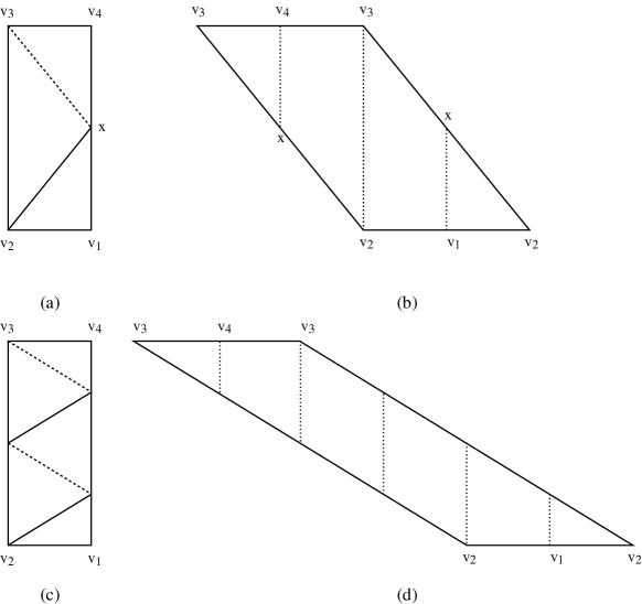
Figure 5: (a)Doubly covered rectangle with cut path; (b) Unfolding. (c-d): Another cut path and its unfolding.

This example can be modified to a nondegenerate “sliver” tetrahedron by perturbing one vertex to lie slightly out of the plane of the other three. $\Box$

Fig. 5(c-d) shows that we cannot even bound the length of a geodesic arc of $T_{C}$.

One immediate corollary of Lemma 4.1 is that cuts need not follow polytope edges (which are all shortest paths), i.e., not every convex unfolding is an edge unfolding.

4.2 Necessary Conditions: Sharp Vertices

We define a vertex of a polytope to be sharp if it has curvature $\geq\pi$, and round if its curvature is $<\pi$. The following theorem gives a simple necessary condition for a polytope to have a convex unfolding. We employ this fact implied by the Gauss-Bonnet theorem:

Fact 4.1

The sum of the curvatures of all the vertices of a polytope is exactly $4\pi$.

Theorem 4.2

If a polytope $Q$ has a convex unfolding via a cut tree $T_{C}$, then each leaf of $T_{C}$ is at a sharp vertex. Moreover, $Q$ must have at least two sharp vertices.

Proof: Let $P$ be a convex polygon to which $Q$ unfolds via cut tree $T_{C}$. By Lemma 3.1(3), the leaves of $T_{C}$ are at vertices of $Q$. Let $x$ be a leaf of $T_{C}$, at a vertex $v$ with curvature ${\gamma}(v)={\gamma}$. Point $x\in{\partial Q}$ corresponds to a unique point $y\in{\partial P}$ by Lemma 3.1(4). The internal angle at $y$ in $P$ is $2\pi-{\gamma}$. Because $P$ is convex, we must have

$$2\pi-{\gamma}\leq\pi$$

and so ${\gamma}(v)\geq\pi$. Thus $v$ is sharp. Because $T_{C}$ must have at least two distinct leaves, the lemma follows. $\Box$

Corollary 4.3

Of the five Platonic solids, only the regular tetrahedron has a convex unfolding.

Proof: The curvatures at the vertices of the solids are:

$$2\pi-3(\pi/3)= \pi$$

$$2\pi-3(\pi/2)= \pi/2 <\pi$$

$$2\pi-4(\pi/3)= 2\pi/3 <\pi$$

$$2\pi-3(3\pi/5)= \pi/5 <\pi$$

$$2\pi-5(\pi/3)= \pi/3 <\pi$$

Only the tetrahedron has sharp vertices. $\Box$

We next show that two natural extensions of the previous results fail.

Lemma 4.4

There is a tetrahedron with no convex unfolding.

Proof: Let $Q_{1}$ be a tetrahedron whose vertices $v_{1},v_{2},v_{3}$ form an equilateral triangle base in the $xy$-plane, with apex $v_{4}$ centered at a great height $z$ above. See Fig. 7. Let ${\gamma}_{i}$ be the curvature of vertex $v_{i}$. If the face angle of each triangle incident to $v_{4}$ is ${\epsilon}$, then ${\gamma}_{4}=2\pi-3{\epsilon}$, and ${\gamma}_{i}$ for $i=1,2,3$ is

$$2\pi-[\pi/3+2(\pi-{\epsilon}/2)]=2\pi/3+{\epsilon}$$

Choosing $z$ large makes ${\epsilon}$ small, and then $Q_{1}$ has just one sharp vertex. Theorem 4.2 then establishes the claim. $\Box$

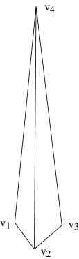
Figure 6: A tetrahedron $Q_{1}$ without a convex unfolding.

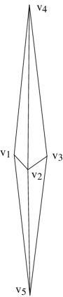
Figure 7: A polytope $Q_{2}$ with two sharp vertices but no convex unfolding.

Lemma 4.5

There is a polytope with two sharp vertices but with no convex unfolding.

Proof: Our proof of this lemma is less straightforward, although the example is simple. Let $Q_{2}$ be the polytope formed by joining two copies of $Q_{1}$ from Lemma 4.4 at their bases, as shown in Fig. 7. $Q_{2}$ is a $5$-vertex polytope, with vertices $v_{1},\ldots,v_{4}$ as in $Q_{1}$, and $v_{5}$ the reflection of $v_{4}$ in the central triangle $C=\triangle v_{1}v_{2}v_{3}$. Again let ${\epsilon}$ be the face angle incident to $v_{4}$ (and symmetrically $v_{5}$), and choose ${\epsilon}$ small so that only $v_{4}$ and $v_{5}$ are sharp vertices.

By Lemma 3.1(3), if $Q_{2}$ has a convex unfolding, the cut tree must be a path with its two leaves at the two sharp vertices. By Lemma 3.1(5), the path must be composed of geodesics. We now analyze the geodesics starting at $v_{5}$ and show that there can be no piecewise simple geodesic path that passes through all the vertices of $Q_{2}$.

We group the geodesics starting at $v_{5}$ into three classes:

1. The three geodesics that pass through a midpoint of an edge of triangle $C$. Each of these passes through $v_{4}$ before encountering any of the other vertices, and so cannot serve as the cut path.

2. The three geodesics that pass through a vertex of $C$. Because these vertices have low curvature ($2{\epsilon}$), the geodesic must emerge nearly headed toward $v_{4}$: it cannot turn to hit another vertex of $C$ without creating a reflex angle in the unfolding. If the geodesic goes directly to $v_{4}$, then again this cannot serve as the cut path. So it must head towards $v_{4}$ but miss it. We group this type of geodesic with the third class.

3. Geodesics that pass though an interior point of an edge of $C$, but not the midpoint. These geodesics all head toward $v_{4}$ but miss it.

We now argue that all the geodesics in the third class (the only remaining candidates) self-intersect after looping around $v_{4}$. This will then establish the lemma.

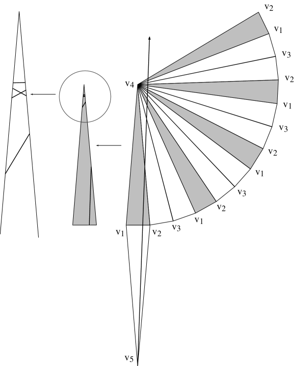
Figure 8: A geodesic from $v_{5}$ that passes by $v_{4}$. The path of the geodesic on $\triangle v_{1}v_{2}v_{4}$ is shown to the left.

An unfolding of a typical geodesic is shown in Fig. 8. By choosing ${\epsilon}$ small, we can arrange that every such geodesic crosses several unfoldings of the three faces incident to $v_{4}$ before returning back down to triangle $C$. As can be seen from the copy of face $\triangle v_{1}v_{2}v_{4}$ to the side, the path crosses each face several times slanting one way, and then returns slanting the other way. In the vicinity of the closest approach to $v_{4}$, the path must self-cross. We now establish this more formally.

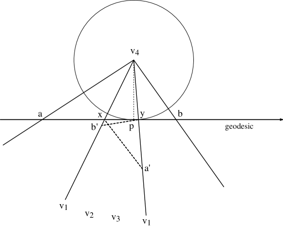
Figure 9: $xa^{\prime}$ and $yb^{\prime}$ necessarily cross below the point $p$ of the geodesic closest to $v_{4}$.

Consider the unfolding of the three faces incident to $v_{4}$ (now viewed as a unit) that includes the point $p$ of closest approach between the geodesic and $v_{4}$; see Fig. 9. Let the geodesic cross the edge $v_{1}v_{4}$ at points $a$, $x$, $y$, and $b$ in that order, with $xy$ including $p$. Then $|v_{4}b|>|v_{4}x|$ and $|v_{4}a|>|v_{4}y|$, because the distance from $v_{4}$ monotonically increases on either side of $p$. Thus the images $a^{\prime}$ and $b^{\prime}$ of $a$ and $b$ must fall below $y$ and $x$ respectively in the figure. Thus the geodesic must cross somewhere in the stretch immediately before and after the closest approach.

All we need for this argument to hold in general is for the geodesic to cross three complete unfoldings of the three faces incident to $v_{4}$ before returning to the lower half of $Q_{2}$. But this is easily arranged by choosing ${\epsilon}$ small.

We have shown that no geodesic starting from $v_{5}$ may serve as a cut path for a convex unfolding. Therefore $Q_{2}$ has no convex unfolding. $\Box$

4.3 Necessary Conditions: Combinatorial Structure

We now study the combinatorial structure of cut trees that lead to convex unfoldings. The following theorem is due to Shephard [She75], although under different assumptions and with a different proof.

Theorem 4.6

If a polytope $Q$ of $n\neq 4$ vertices has a convex unfolding, then the corresponding cut tree $T_{C}$ has two or three leaves: it is either a path, or a ‘Y’ (a single degree-$3$ node). If $n=4$, then additionally it may have four leaves, and have the combinatorial structure of ‘+’ (a single degree-$4$ node), or two degree-$3$ nodes connected by an edge, which we will call a ‘I’.

Proof: Let the cut tree $T_{C}$ unfold $Q$ to a convex polygon. By Theorem 4.2, each leaf of $T_{C}$ must be at a sharp vertex $v$, and so have curvature ${\gamma}(v)\geq\pi$. If $T_{C}$ has more than four leaves $v$ (and therefore $n>4$, i.e., we are in the $n\neq 4$ case of the theorem claim), $\sum_{v}{\gamma}(v)>4\pi$, which violates the Gauss-Bonnet theorem. Therefore $T_{C}$ has no more than four leaves. If $T_{C}$ has just two or three leaves, then the only possible combinatorial structures for $T_{C}$ are the two claimed in the theorem: a path, and a ‘Y’. (Note that it is possible that $n=3$, when $Q$ is a doubly-covered triangle.)

So assume that $T_{C}$ has exactly four leaves. Because each leaf vertex is sharp, $\sum_{v}{\gamma}(v)\geq 4\pi$; on the other hand, we know the sum over all vertices is equal $4\pi$. Therefore we know that each leaf has curvature exactly $\pi$ and that the leaves of $T_{C}$ are at the only vertices of $Q$. Thus $n=4$ and $Q$ is a tetrahedron. The only additional possible combinatorial structures for a tree with four leaves are the two claimed in the theorem: a ‘+’ and a ‘I’. Note that in both these cases, the internal node(s) of $T_{C}$ are not at vertices of $Q$. $\Box$

A simple example of the ‘I’ possibility is shown in Fig. 10. If the rectangle is modified to become a square, the ‘I’ becomes a ‘+’.

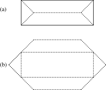
Figure 10: A doubly-covered rectangle unfolds with a ‘I’ cut tree whose leaves are the four rectangle corners. Note all four rectangle corners are fold vertices.

5 Counting Foldings: Gluing Trees

In this section we move beyond Lemma 2.1, which shows that every convex polygon folds to a polytope, and explore how many different ways there are to fold a given polygon, as measured by the number of combinatorially distinct Aleksandrov gluing trees. In Section 6 we count instead the number of distinct polytopes that might be produced from a given polygon. In both cases, we will also examine the restriction to convex polygons, which not surprisingly yields sharper results.

5.1 Unfoldable Polygons

We start with a natural and easily proved claim:

Lemma 5.1

Some polygons cannot be folded to any polytope.

Proof: Consider the polygon $P$ shown in Fig. 11.

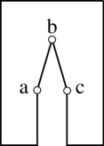
Figure 11: An unfoldable polygon.

$P$ has three consecutive reflex vertices $(a,b,c)$, with the exterior angle ${\beta}$ at $b$ small. All other vertices are convex, with interior angles strictly larger than ${\beta}$.

Either the gluing “zips” at $b$, leaving $b$ a leaf of $T_{G}$, or some other point(s) of ${\partial P}$ glue to $b$. The first possibility forces $a$ to glue to $c$, exceeding $2\pi$ there; so this gluing is not Aleksandrov. The second possibility cannot occur with $P$, because no point of ${\partial P}$ has small enough internal angle to fit at $b$. Thus there is no Aleksandrov gluing of $P$. $\Box$

It is natural to wonder what the chances are that a random polygon could fold to a polytope. This is difficult to answer without a precise definition of “random,” but we feel any reasonable definition would lead to the same answer:

Conjecture 5.1

The probability that a random polygon of $n$ vertices can fold to a polytope approaches $0$ as $n\rightarrow\infty$.

Proof: (Sketch.) Assume that random polygons on $n$ vertices satisfy two properties:

1. The distribution of the polygon angles approaches the uniform distribution on the interval $(0,2\pi)$ as $n\rightarrow\infty$. In particular, the number of reflex and convex vertices approaches balance.

2. The distribution of polygon edge lengths approaches some continuous density distribution.

For large $n$, we expect $P$ to have $r=n/2$ reflex vertices. Each of these reflex vertices $a$ faces one of two fates in the gluing tree: either it becomes a leaf by “zipping” at $a$; or at least one convex vertex $b$ (of sufficiently small angle) is glued to $a$. The number of reflex vertices that can be zipped is limited by Fact 4.1: if $a$ has angle ${\alpha}$, zipping there adds $2\pi-{\alpha}$ to the curvature; but the total curvature is limited to $4\pi$. Suppose we zip the largest $k$ angles out of the $r$ reflex vertices (the largest angles increment the curvature the least). Then one can compute that, under the uniform angle distribution assumption, these $k$ angles have an expected curvature sum of

$$\frac{1}{2}\frac{\pi}{r}k^{2}\;.$$ (1)

(For example, for $r=100$, the largest $k=10$ have an expected curvature sum of $\pi/2$.) Limiting this to $4\pi$ implies that the expected maximum number of reflex vertices that can be zipped without exceeding $4\pi$ curvature is

$$k\leq 2\sqrt{2r}=2\sqrt{n}\;.$$ (2)

(For example, for $r=1000$ reflex vertices, the largest $k=89$ lead to a curvature of $\approx 4\pi$.) Thus, at most a small portion of the reflex vertices can be zipped; the remainder (expected number: $n/2-2\sqrt{n}$) must be glued to convex vertices. We now show that this gluing is not in general possible.

Let $a$ be a reflex vertex with angle ${\alpha}$, and $b$ a convex vertex whose angle ${\beta}$ satisfies ${\beta}\leq 2\pi-{\alpha}$, so that $b$ can glue to $a$. It could be that this gluing forces one or more reflex vertices adjacent to $a$ or $b$ to glue to edges incident to $a$ or $b$, in which case the gluing is not possible (i.e., it is not an Aleksandrov gluing). If the adjacent vertices are convex, and/or the edge lengths are such that the gluing is Aleksandrov, then, in general, two new reflex vertices are created, as is illustrated in Fig. 12.

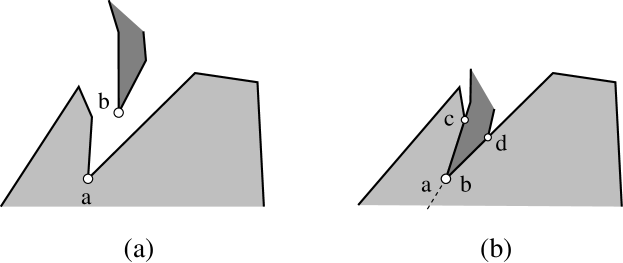
Figure 12: (a) Reflex vertex $a$, convex vertex $b$; (b) Two new reflex vertices produced by gluing $b$ to $a$.

To be more precise, let $A=|aa_{1}|$ be the length of the edge incident to $a$ which is glued to the length $B=|bb_{1}|$ of an edge incident to $b$. If $A>B$ and $b_{1}$ is reflex, the gluing is not Aleksandrov; but if $b_{1}$ is convex, a new reflex vertex is created at $b_{1}$. Symmetrically, if $B>A$ and $a_{1}$ is reflex, the gluing is not possible; but if $a_{1}$ is convex, a new reflex vertex is created at $a_{1}$. The only circumstance in which the gluing is Aleksandrov and a new reflex vertex is not created is when $A=B$ and both $a_{1}$ and $b_{1}$ are convex with an angle sum of no more than $\pi$.

Under the assumption that the edge lengths approach some continuous distribution, the probability that two lengths match exactly approaches $0$. Thus we conclude that gluing convex vertices to reflex vertices does not remove reflex vertices, but rather creates new ones in shorter polygonal chains, one new reflex vertex in each of the two chains produced by the gluing. Note that gluing several convex vertices to one reflex vertex does not change matters: we can view the first convex vertex as simply leaving a reflex remainder, and argue as above.

Thus, any gluing of a random polygon for large $n$ will lead to shorter and and shorter chains “pinched” between reflex-convex gluings, each of which will contain at least one reflex vertex (actually, two reflex vertices for those pinched on both sides). Eventually these chains reach the point where either there are no convex vertices that fit into the reflex vertex gap, or there are no convex vertices at all. In either case, the chain cannot be glued: the reflex vertex would have to glue to a point interior to an edge, violating the Aleksandrov condition that no point have more than $2\pi$ glued angle. $\Box$

The proof above hinges on the unlikeliness of matching edge lengths. It is therefore natural to wonder if the same result holds for polygons all of whose edge lengths are the same. Again we believe it does:

Conjecture 5.2

The probability that a random polygon of $n$ vertices, all of whose edges have unit length, can fold to a polytope, approaches $0$ as $n\rightarrow\infty$.

Proof: (Sketch.) Assume a model of random polygons such that the angles are probabilistically independent and uniformly distributed in $(0,2\pi)$ as $n\rightarrow\infty$. The restriction to unit edge lengths means that all gluings are vertex to vertex (no vertex is ever glued to the interior of an edge). The gluing is Aleksandrov iff the angles glued together sum to at most $2\pi$ everywhere.

Consider gluing two vertices to one another. Because their angles are independent, the chance that the gluing is legal is $1/2$ (the sum of their distributions is uniform between $0$ and $4\pi$). Gluing $k$ pairs then has a $1/2^{k}$ chance of being Aleksandrov.

As in the above proof sketch, the gluing tree cannot have too many leaves. Zipping just $2\sqrt{n}$ reflex vertices uses up all $4\pi$ of curvature. So the number of leaves is only about $2\sqrt{n}$. As we will see in Theorem 5.11 below, specifying a “source” for each leaf pins down the whole tree structure. So by selecting $4\sqrt{n}$ vertices for the leaves and their sources, the gluing tree is determined.

Therefore we should compare the number of different gluing trees,

$$\left(\begin{array}[]{c}n\\ 4\sqrt{n}\end{array}\right)$$ (3)

to the probability that each one is Aleksandrov,

$$\frac{1}{2^{n-4\sqrt{n}}}$$ (4)

Note here we conservatively only concern ourselves with degree-$2$ vertex-to-vertex gluings; junctions of degree $d>2$ have a lower probability of summing to no more than $2\pi$. We also ignore the change to the angle distribution caused by the removal of the leaf vertices.

Using Stirling’s approximation shows that the $\log$ of Eq. (3) grows as $2\sqrt{n}\log n$; but the $\log$ of Eq. (4) grows as $n$. So their ratio approaches $0$ as $n\rightarrow\infty$. $\Box$

We leave these results on random polygons as conjectures, as it would require a more precise definition of what constitutes a random polygon, and more careful probabilistic analyses, to establish them formally.

5.2 Lower Bound: Exponential Number of Gluing Trees

In contrast to the likely paucity of foldable polygons, some polygons generate many foldings.

Theorem 5.2

For any even $n$, there is a polygon $P$ of $n$ vertices that has $2^{\Omega(n)}$ combinatorially distinct Aleksandrov gluings.

Proof: The polygon $P$ is illustrated in Fig. 13(a).

Figure 13: (a) Star polygon $P$, $m=16$, $n^{\prime}=32$, $n=34$. (b) Base gluing tree. (c) A gluing tree after several contractions.

It is a centrally symmetric star, with $m$ vertices, $m$ even, with a small convex angle ${\alpha}\approx 0$, alternating with $m$ vertices with large reflex angle ${\beta}<2\pi$. All edges have the same (say, unit) length. We call this an $m$-star. We first specify the constraints on ${\alpha}$ and ${\beta}$.

$P$ has $n^{\prime}=2m$ vertices (ignoring $x$ and $y$, to be described shortly). So $m({\alpha}+{\beta})=(n^{\prime}-2)\pi$, which implies that

$${\alpha}+{\beta}=(1-\frac{1}{m})2\pi\;.$$ (5)

We choose ${\alpha}$ small enough so that $m$ copies of ${\alpha}$ can join with one of ${\beta}$ and still be less than $2\pi$:

$$m{\alpha}+{\beta}<2\pi\;.$$ (6)

Substituting this relationship into Eq. (5) and solving for ${\alpha}$ yields:

$${\alpha}<\frac{2\pi}{m(m-1)}\;.$$ (7)

Now we add two vertices $x$ and $y$ at the midpoints of edges, symmetrically placed so that $y$ is half the perimeter around ${\partial P}$ from $x$. Let $n=n^{\prime}+2$ be the total number of vertices of $P$.

The “base” gluing tree is illustrated in Fig. 13(b). $x$ and $y$ are fold vertices of the gluing. Otherwise, each ${\alpha}$ is matched with a ${\beta}$. Because all edge lengths are the same, and because ${\alpha}+{\beta}<2\pi$ by Eq. (5), this path is an Aleksandrov gluing. We label it $T_{00\cdots 0,00\cdots 0}$, where $m/2$ zeros $00\cdots 0$ represent the top chain, and another $m/2$ zeros represent the bottom chain.

The other gluing trees are obtained via “contractions” of the base tree. A contraction makes any particular ${\beta}$-vertex not adjacent to $x$ or $y$ a leaf of the tree by gluing its two adjacent ${\alpha}$-vertices together. Label a ${\beta}$-vertex $0$ or $1$ depending on whether it is uncontracted or contracted respectively. Then a series of contractions can be identified with a binary string. For example, Fig. 13(c) displays the tree $T_{010100\cdots,00110\cdots 0}$. Note that $k$ adjacent contractions result in $2k$ ${\alpha}$-vertices glued together.

We now claim that if the number of contractions in the top chain is the same as the number in the bottom chain (call such a series of contractions balanced), the resulting tree represents an Aleksandrov gluing. Fix the position of $x$ to the left, and contract leftwards, as in Fig. 13(c). Then it is evident that the alternating “parity” pattern of ${\alpha}$’s and ${\beta}$’s is not changed by contractions. Ignoring the arcs attached to the central path, each contraction replaces ${\alpha}\rightarrow 2{\alpha}$, and shortens the path by $2$ units. Because the contraction shortens by an even number of units, it does not affect the parity pattern. If the top and bottom chains are contracted the same number of times (twice each in (c) of the figure), then their lengths are the same.

Thus after a balanced series of contractions, we have a number of ${\beta}$-leaves, and gluings of $2k$ ${\alpha}$-vertices to one ${\beta}$-vertex. The ${\beta}$-leaves are legal gluings because ${\beta}<2\pi$. Because there are $m/2-1$ contractible ${\beta}$-vertices in each chain, the longest series of adjacent contractions is $m/2-1$. So $k\leq m/2-1$, and $2k<m$. Eq. (6) then shows that each gluing produces less than $2\pi$ angle, and so is Aleksandrov.

Finally, we bound the number of gluings. There are $2^{m/2-1}$ binary numbers of $m/2-1$ bits. Thus there are this many ways to contract the top chain. The bottom chain must be contracted with the same number of $1$’s for a balanced series. Rather than count this explicitly, we simply note that $P$ has at least $2^{m/2-1}$ Aleksandrov gluings, and because $P$ has $n=n^{\prime}+2=2m+2$ vertices, $\Omega(2^{m/2-1})=\Omega(2^{(n-6)/4})=2^{\Omega(n)}$. $\Box$

Figure 14: Six gluing patterns for a $4$-star.

Fig. 14 shows six gluings of a $4$-star. The first two in the top row correspond to the perimeter-halving construction used in the proof. By Aleksandrov’s theorem, each corresponds to a unique polytope, but as mentioned in Section 2, we do not know how to compute the 3D structure of these polytopes. Nevertheless, our hand-exploration suggest that all fold to noncongruent polytopes, each with the combinatorial structure of the regular octahedron. Two of our conjectured crease patterns are shown in Fig. 15.

Figure 15: Conjectured crease patterns for the first two gluing patterns in the top row of Fig. 14. [Constructions performed in Cinderella.]

5.3 Upper Bound: Few Leaves

Our goal is now to provide upper bounds on the number of gluings, both for arbitary polygons and for convex polygons. Both will rely on upper bounds for gluing trees with a small number of leaves. Let a gluing tree $T_{G}$ have ${\lambda}$ leaves. In this section, we prove results for ${\lambda}=2$ and ${\lambda}=3$. We then use these to obtain a general upper bound in Section 5.4, and a bound for convex polygons in Section 5.6. In between, we summarize the structural properties of gluing trees in Section 5.5.

It will sometimes be easier to work with “gluing instructions” rather than with gluing trees. Toward that end, we define the combinatorial type of a gluing. Again let polgyon $P$ have vertices $v_{i}$ and edges $e_{i}$, labeled counterclockwise, The combinatorial type ${\Gamma}_{G}$ of a gluing $G$ specifies to which vertex or edge of $P$ each vertex of $P$ glues via a set of ordered pairs: ${\Gamma}_{G}=\{(v_{i},z_{j})\}$, where $z_{j}$ is either $v_{j}$ or $e_{j}$, the first element $j$ to which $v_{i}$ glues counterclockwise around ${\partial P}$. If $v_{i}$ is a leaf of the cut tree, then the pair $(v_{i},v_{i})$ is included; otherwise $v_{i}$ must glue to an element different from itself. For example, the combinatorial type of the gluing illustrated earlier in Fig. 3a is

$$\{(v_{1},v_{3}),(v_{2},v_{2}),(v_{3},e_{3})\}$$

We now prove that the combinatorial type of a gluing determines the gluing tree.

Lemma 5.3

The combinatorial type ${\Gamma}_{G}$ of a gluing $G$ determines the gluing tree $T_{G}$.

Proof: A node of degree $2$ of $T_{G}$ is directly labeled in ${\Gamma}_{G}$ as either $(v_{i},v_{j})$ or $(v_{i},e_{j})$. It is only nodes of degree $\neq 2$ for which $T_{G}$ contains information not immediately supplied by ${\Gamma}_{G}$. Nodes of degree $1$ (leaves) of $T_{G}$ correspond to two possible types of gluings: either $(v_{i},v_{i})$, which are directly labeled in ${\Gamma}_{G}$, or fold vertices, a vertex produced by folding at a point $x$ in the interior of an edge $e_{j}$. (Cf. Fig. 1 for an example of fold vertices.) Fold vertices can be identified in ${\Gamma}_{G}$ as gluings of $v_{i}$ to either $e_{i}$ or $e_{i-1}$: gluing to an incident edge necessarily implies a fold vertex on that edge. Or $v_{i}$ can be glued to the next vertex, folding the edge in half. In Fig. 3, the pair $(v_{3},e_{3})$ identifies fold vertex $x$ as labeled with $e_{3}$; that $v_{1}$ also glues to incident edge $e_{3}$ is known after the degree $3$ node’s labels are determined.

Nodes of degree $d>2$ in $T_{G}$ have $d$ labels. Because every such node can involve at most one edge (because two edges glued to a point already gives an angle of $2\pi$ there, and the other elements glued to the same point would cause the angle sum to exceed this), the labels can be gathered by following the gluings counterclockwise:

$$(v_{i_{1}},v_{i_{2}}),(v_{i_{2}},v_{i_{3}}),\ldots,(v_{i_{d{-}2}},v_{i_{d{-}1}}),(v_{i_{d{-}1}},e_{j})\,.$$

In Fig. 3, the node at point $z$ has labels $\{v_{1},v_{3},e_{3}\}$, which can be identified from the pairs $(v_{1},v_{3}),(v_{3},e_{3})$ of ${\Gamma}_{G}$. $\Box$

This lemma permits us to count gluing trees by counting combinatorial types of gluings.

Lemma 5.4

A polygon $P$ of $n$ vertices has $\Theta(n^{2})$ different gluing trees of two leaves, i.e., paths.

Proof: View ${\partial P}$ as rolling continuously between the two leaves $x$ and $y$, like a conveyor belt or tank tread. Each specific position corresponds to a perimeter-halving gluing $G$ (Fig. 1). The combinatorial type ${\Gamma}_{G}$ changes each time a vertex $v_{i}$ either passes another vertex $v_{j}$, or becomes the leaf $x$ or $y$. Each such event corresponds to two distinct types: the type at the event, and the type just beyond it: e.g., $(v_{i},v_{j})$ and $(v_{i},e_{j})$. So counting events undercounts by half. If we count the possible pairs $(v_{i},v_{j})$ for all $i\neq j$, we will double count each type: the event $(v_{i},v_{j})$ leads to the same type as $(v_{j},v_{i})$. The undercount by half and overcount by double cancel; thus $n(n-1)$ is the number of types without a vertex at a leaf. Adding in the $n$ possible $(v_{i},v_{i})$ events, each of which leads to two types, yields an upper bound of $n(n-1)+2n=O(n^{2})$ on the number of combinatorial types.

A lower bound of $\Omega(n^{2})$ is achieved by the example illustrated in Fig. 16(a). Here $n/2$ vertices of $P$ are closely spaced within a length $L$ of ${\partial P}$, and $n/2$ vertices are spread out by more than $L$ between each adjacent pair. Then each of the latter vertices (on the lower belt in the figure) can be placed between each pair of the former vertices (on the upper belt), yielding $n^{2}/4$ distinct types. This example can be realized geometrically by making the internal angle at each vertex nearly $\pi$, i.e., by a convex polyon that approximates a circle.

Lemma 5.3 shows that the bound just obtained of $\Theta(n^{2})$ on the number of combinatorial types applies as well to the number of gluing trees. $\Box$

Figure 16: (a) $\Omega(n^{2})$ combinatorial types can be achieved by rolling this perimeter “belt”; (b) There are only $O(n)$ possible disjoint vv-pairings.

Lemma 5.5

A polygon $P$ of $n$ vertices folds to at most $O(n^{4})$ different gluing trees of three leaves, i.e., ‘Y’s.

Proof: Observe that the degree-$3$ node of the ‘Y’ is either comprised by the gluing two vertices and an edge together (call this type-vve), or three vertices (type-vvv). It is not possible to glue two or more edges together without violating the $\leq 2\pi$ angle restriction of an Aleksandrov gluing.

There are $O(n^{3})$ possible type-vvv nodes for the ‘Y’. Once this type of node is specified, the entire gluing tree is determined, so this bounds the number of ‘Y’s with type-vvv nodes. Now consider type-vve nodes. There are $O(n^{2})$ possible vv-gluings, which determine one branch of the ‘Y’. The remainder of the ‘Y’ can be viewed as a path between its leaves; essentially this view corresponds to a conveyor belt with an appendage. Applying Lemma 5.4 yields a bound of $O(n^{4})$.

$\Box$

We leave open the question of whether this bound is tight. We will improve it for convex polygons in Section 5.6.

5.3.1 Four Fold-Point Gluing Trees

We now embark on a study of a special case that will play two roles: in the proof of our main combinatorial upper bound, Theorem 5.11, and in counting noncongruent polytopes in Section 6. Define a four fold-point gluing tree to be a gluing tree with (at least) four leaves, each fold points, i.e., creases in the interior of polygon edges leading to polytope vertices of curvature $\pi$. We have already encountered one such tree in Fig. 4(b). We start with this straightforward lemma.

Lemma 5.6

A four fold-point gluing tree must have exactly four leaves, and so have combinatorial structure ‘+’ or ‘I’.

Proof: Because each fold point leads to a vertex of the resulting polytope $Q$ which has curvature $\pi$, Fact 4.1 implies that all the curvature of the polytope is at the four fold vertices. Thus all vertices of $P$ must glue to points that have total angle $2\pi$, so that the curvature there is zero.

A leaf of a gluing tree cannot have zero curvature. This is because a leaf is either a fold point (curvature $\pi$) or a “zipped” polygon vertex $v$. The only way to achieve zero curvature at a zipped vertex is to have an internal polygon angle at $v$ of $2\pi$. But this violates simplicity of $P$: all internal angles are strictly less than $2\pi$.

Therefore, a four-fold gluing tree must have exactly four leaves. So there are only two possible combinatorial structures: ‘+’ and ‘I’ (as in Lemma 3.1). $\Box$

Before counting the number of gluing trees, we detail one example that will be the basis for the remainder of our analysis. Start with an $L\times W$ rectangle $P$, and fold it as follows. Glue the two opposite edges of length $W$ together to form a cylinder. Now glue the bottom rim of the cylinder to itself by creasing at two diametrically opposed points $x_{1}$ and $y_{1}$. Similarly glue the top rim to itself by creasing at two points $x_{2}$ and $y_{2}$. The gluing tree is of structure ‘I’: see Fig. 17.

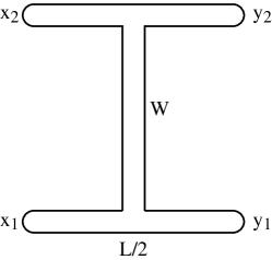
Figure 17: ‘I’ gluing tree for an $L\times W$ rectangle.

It is easy to see this is an Aleksandrov gluing. Note both internal nodes of the gluing tree glue two $\pi/2$ rectangle corners to the interior of an $L$-edge; so the angle sum there is $2\pi$. The gluing is Aleksandrov even if the crease points on the top and bottom are not located at corresponding points on their rims. In particular, identify the points $x_{i}$ with their distance from the rectangle corner to the left. If $x_{1}=x_{2}$, then the crease points correspond, and the gluing produces a flat, $L/2\times W$ rectangle. If $x_{1}\neq x_{2}$, the gluing is still Aleksandrov, but the “twist” in the gluing results in a nondegenerate tetrahedron, with all vertices of curvature $\pi$. Let $x=|x_{2}-x_{1}|$ characterize amount of the twist, with $x=0$ representing no twist.

Because the $1$-skeleton of a tetrahedron is combinatorially $K_{4}$, each vertex is adjacent to all the others via polytope edges. This makes it trivial to decide the structure of the polytope $Q_{x}$ created by this rectangle gluing with twist $x$. The six distances between pairs of vertices are easily computed from the gluing, and each represents an edge length. These six lengths uniquely determine the 3D shape of the tetrahedron. It is not difficult to compute 3D vertex coordinates from the six lengths, and we have written code for this computation. An example is shown in Fig. 18. Here a $2\times 2$ rectangle is folded with a variety of different twists $x$. For both $x=0$ and $x=1$, the result is a flat $1\times 2$ rectangle, with a smooth interpolation between for $0<x<1$.

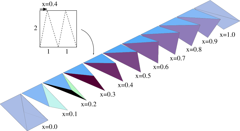
Figure 18: Tetrahedra formed by folding a rectangle according to the gluing tree shown in Fig. 17.

We have proven this lemma:

Lemma 5.7

Any rectangle may fold via a ‘I’ gluing tree to a uncountably infinite number of noncongruent tetrahedra.

Proof: Two tetrahedra with different edges lengths are not congruent. The edge lengths of $Q_{x}$ for twist $x$ are $L/2$ (twice), $u(x)=\sqrt{x^{2}+W^{2}}$ (twice), and $v(x)=\sqrt{(1-x)^{2}+W^{2}}$ (twice). For $a\neq b$, $u(a)\neq u(b)$; and for $x<L/4$, $u(x)\neq v(x)$. Thus the number of noncongruent tetrahedra is at least the number of distinct $x\in[0,L/4)$, which is nondenumerable. $\Box$

We return now to the task of upper-bounding the number of four fold-point gluing trees possible for a polygon of $n$ vertices. Although we do not at this point have tight bounds, they suffice for our purposes in the next section.

Define a conveyor belt (or just belt)  in a gluing tree to be a path between two leaf fold points. Let a belt have fold points $x$ and $y$, with $x$ an interior point of edge $e$. A belt can roll if there is a nonzero-length interval $I\subset e$ such that for every $x\in I$, the belt folded at $x$ is an Aleksandrov gluing. A belt could instead have a finite number of distinct gluings, perhaps just one. We first show that rolling belts must be vertex-free in four fold-point trees.

Lemma 5.8

A rolling belt in a four fold-point tree $T$ cannot contain any vertices except those at the attachment points to other branches of $T$.

Proof: Suppose to the contrary that a rolling belt contains at least one vertex $v$ in its interior, i.e., not at an attachment point. Because under our definition, all vertices of $P$ are essential, the internal angle at $v$ is different from $\pi$. Let $x\in I$ be a particular fold point that determines the gluing of the belt. In this position, $v$ must match up with another vertex $v^{\prime}$ with supplementary angle. Rolling the belt in a neighborhood of $x$ breaks the match, leaving both $v$ and $v^{\prime}$ glued to points internal to an edge. At these points, the curvature is greater than zero, violating the fact that all curvature at a four fold-point gluing are concentrated at the leaves. $\Box$

Note that the angles at the attachment points must be $\pi$.

Lemma 5.9

A belt in a four-fold gluing tree $T$ has at most $O(n)$ combinatorially distinct gluings.

Proof: Let $B$ be a belt with attachment points $a$ and $b$. Note that because each attachment point is an internal node of $T$, the limited structural possibilities established in Lemma 5.6 allow only one or two attachment points. Consider two cases:

1. $B$ can roll. Then by Lemma 5.8, $B$ contains no internal vertices. Thus its only vertices are at $a$ and $b$. Rolling can produce just two combinatorially distinct positions of the belt.

2. $B$ cannot roll. Then $B$ can assume a finite number of possible positions. Define a kink in $B$ to be either a vertex, or an attachment point at which the angle is different from $\pi$, composed of two glued vertices. The kinks must match up in pairs. Matching one pair forces the remaining matches. Thus This can be seen by distributing the kinks around a topological circle representing $B$. Once one chord $v_{1}v_{i}$ is drawn in this circle, all other chords are forced by the pairwise matching requirement. Because there are only $m-1<n$ choices for the mate for $v_{1}$, $B$ has only $O(n)$ legal gluings.

$\Box$

Lemma 5.10

The number of four fold-point gluing trees for a polygon of $n$ vertices is $\Omega(n^{2})$ and $O(n^{4})$.

Proof: The lower bound is established by a variation on the foldings of a rectangle to tetrahedra (Fig. 18). The idea is to make each of the two conveyor belts in a ‘I’ structure (Fig. 17) realize $\Omega(n)$ gluings independently. This can be accomplished by alternating supplementary angles along the belt at equal intervals. This is illustrated in Fig. 19 with angles $\pi/2$ and $3\pi/2$. The figure illustrates one possible folding; the fold points are midpoints of edges. The tetrahedra produced are the same as that obtained by folding a rectangle: the “teeth” mesh seamlessly.

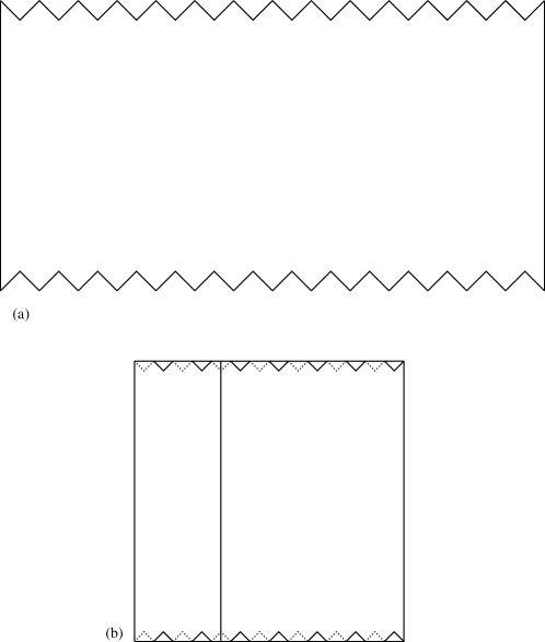
Figure 19: (a) Polygon $P$; (b) One four fold-point gluing. The dashed lines indicate tips of front teeth bent over and glued behind.

For the upper bound, Lemma 5.6 restricts the structures to ‘+’ and ‘I’.

1. ‘+’. Here we rely on the crude $O(n^{4})$ bound determined by the four vertices, or three vertices and one edge, glued together to form the interior node of $T_{G}$. This fixes the combinatorial type of the gluing, which by Lemma 5.3 determines $T_{G}$.

2. ‘I’. Let $a$ and $b$ be the upper and lower nodes of the ‘I’. There are two cases to consider for the upper node:

   1. $a$ is of type ‘vv’: vertices $v_{i}$ and $v_{j}$ glue to form the belt attachment point. Then the path from $a$ to $b$ is determined by the requirement that the curvature must be zero at each point: the two sides “zip” closed from $v_{i}$/$v_{j}$ until the first point at which the curvature is nonzero, which then must be the lower node $b$.

   2. $a$ is of type ‘ve’: vertex $v_{i}$ glues to the interior of edge $e_{j}$ to form the attachment point. The “zipping” down to $b$ is again determined, but this takes more argument. Let $v_{i+1}$ and $v_{j}$ be the two vertices closest to $a$ on the path to $b$. Both of their angles must differ from $\pi$ (because all vertices are essential). They must glue to one another with an angle sum of $2\pi$ (because the curvature must be zero). We want to show that $v_{i}$ cannot “slide” along $e_{j}$ to another position and still result in an Aleksandrov gluing. Sliding $v_{i}$ up $e_{j}$ places $v_{i+1}$ in the interior of $e_{j}$, and sliding $v_{i}$ down places $v_{j}$ in the interior of $e_{i}$, in both cases producing a point of nonzero curvature. Therefore no sliding is possible. Because any respositioning of $v_{i}$ on $e_{j}$ can be viewed as such a sliding, no repositioning is possible.

In both cases there are at most $O(n^{2})$ choices for the constituents glued at $a$. Together with the $O(n^{2})$ bound on the two belts from Lemma 5.9, this establishes the claimed $O(n^{4})$ bound. $\Box$

It seems likely that this lemma could be strengthened:

Conjecture 5.3

The number of four fold-point gluing trees for a polygon of $n$ vertices is $\Theta(n^{2})$.

5.4 Upper Bound: General Case

We finally are positioned to establish an upper bound on the number of gluing trees, as a function of the number leaves.

Theorem 5.11

The number of gluing trees with ${\lambda}$ leaves for a polygon $P$ with $n$ vertices is $O(n^{2{\lambda}-2})$.

Proof: Let $g(n,{\lambda})$ be the number of gluing trees for $P$ that have ${\lambda}$ leaves. The proof is by induction on ${\lambda}$. We know from Lemma 5.6 that at most four leaves can be fold-points. We assume for the general step of the induction that ${\lambda}>4$, and so there is at least one non-fold-point leaf. The base cases for ${\lambda}\leq 4$ will be considered later.

The bound will use one consequence of the angles or curvature of a gluing (described in this paragraph), and one consequence of the matching edge lengths of a gluing (described in the next paragraph). Because a point interior to an edge of $P$ has angle $\pi$, a node of degree $d$ of a gluing tree ($d=1,2,\ldots$) glues together $d$ vertices of $P$ or $d-1$ vertices and one edge of $P$. Apart from this, we will use nothing else about the angles of the polygon, and in fact, our argument will hold more generally for a closed chain of $n$ vertices, with specified edge lengths.

Given a tree $T_{G}$ that is not a path, and a leaf $l$, define the source of $l$ as the first node of degree more than 2 along the (unique) path from $l$ into $T$. The path in $T_{G}$ from $l$ to its source is called the branch of $l$. For a tree $T_{G}$ and a non-fold-point leaf corresponding to polygon vertex $l$, let $s(l)$ be a vertex of $P$ closest to $l$ glued at the source of the leaf. Note that there must be such a vertex, since we cannot glue together two points interior to polygon edges at the source of the leaf. For example, in Fig. 3, $s(v_{2})$ can be $v_{3}$ or $v_{1}$. Note—this is the single consequence of matching edge lengths referred to above—that the pair $(l,s(l))$ determines the portion of $P$’s boundary that is glued together to form the branch of $l$. We can simplify $T$ by cutting off $l$’s branch, resulting in a tree with ${\lambda}-1$ leaves. The corresponding simplification of ${\partial P}$ is to excise the portion of its chain of length $2d(l,s(l))$ centered at $l$, resulting in a closed chain on at most $n-1$ vertices. Since there are $n$ choices for $l$ and at most $n$ choices for $s(l)$ we obtain $g(n,{\lambda})\leq n^{2}g(n-1,{\lambda}-1)$. For the general case there are at most 3 fold leaves, hence: $g(n,{\lambda})\leq n^{2({\lambda}-3)}g(n-({\lambda}-3),3)$.

Lemmas 5.4 and 5.5 established the base cases $g(n,2)=O(n^{2})$ and $g(n,3)=O(n^{4})$. Substituting, this yields

$$g(n,{\lambda})\leq n^{2({\lambda}-3)}O([n-({\lambda}-3)]^{4})$$ (8)

$$= n^{2({\lambda}-3)}O(n^{4})$$ (9)

$$= O(n^{2{\lambda}-2})$$ (10)

It remains to handle the case of ${\lambda}=4$ leaves. We will separate into the cases when at least one of these leaves is not a fold-point leaf, where arguments as above yield $O(n^{6})$, and the case when all 4 vertices are fold leaves. In this case, Lemma 5.10 establishes a bound of $O(n^{4})$, smaller than that claimed by the lemma. $\Box$

Of course because ${\lambda}$ could be $\Omega(n)$, there is no contradiction between this upper bound and the exponential lower bound in Theorem 5.2. We specialize the upper bound to convex polygons in Section 5.6, but first we summarize the structural characteristics of gluing trees we have uncovered.

5.5 Gluing Tree Characterization

Our previous results imply that gluing trees are fundamentally discrete structures, with one or two rolling conveyor belts, and two such belts only in very special circumstances.

Theorem 5.12

Gluing trees satisfy these properties:

1. At any gluing tree point of degree $d\neq 2$, at most one point of ${\partial P}$ in the interior of an edge may be glued, i.e., at most one nonvertex may be glued there.

2. At most four leaves of the gluing tree can be fold points, i.e., points in the interior of an edge of ${\partial P}$. The case of four fold-point leaves is only possible when the tree has exactly four leaves, with the combinatorial structure ‘+’ or ‘I’.

3. A gluing tree can have at most two rolling belts.

4. A gluing tree with two rolling conveyor belts must have the structure ‘I’, and result from folding a polygon that can be viewed as a quadrilateral with two of its opposite edges replaced by complimentary polygonal paths.

Proof:

1. That $d\neq 2$ points of a gluing tree have at most one edge-interior points glued is immediate from the definition of an Aleksandrov gluing, and our insistence that all vertices are essential.

2. The structure of four fold-point trees was established in Lemma 5.6.

3. The definition of “rolling belts” (p. 5.7) implies four fold points, so the constraints from the previous item apply.

4. Two rolling belts cannot be accommodated by the ‘+’ structure, which is determined by the four vertices glued at the central node. So the tree structure must be ‘I’. Lemma 5.8 established that the belts are vertex-free, corresponding to two opposite edges of the quadrilateral. The central path of the ‘I’ must be formed by gluing vertices together whose angle sum is $2\pi$, and they are in this sense complimentary polygonal paths.

$\Box$

Thus a generic gluing tree has one rolling belt, with trees hanging off it, and one of those trees having a fold-point leaf. See Fig. 20.

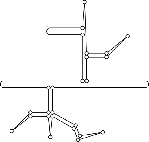
Figure 20: A generic gluing tree: three fold-point leaves (indicated by smooth arcs), two forming a rolling belt. Vertices indicated by open circles.

5.6 Upper Bound: Convex Polygons

For convex polygons we can prove a polynomial upper bound. We first handle the special case of ${\lambda}=4$.

Lemma 5.13

A convex polygon $P$ may fold to gluing trees of four leaves only if it is a quadrilateral, a pentagon, or a hexagon; $P$ may fold to $O(1)$ such gluing trees.

Proof: As in the proof of Theorem 4.6, the two conditions ${\gamma}(v)\geq\pi$ and $\sum_{v}{\gamma}(v)=4\pi$ for the four leaves $v$ of the tree imply that ${\gamma}(v)=\pi$ for each. This implies that the internal angle at $v$ in $P$ is $\pi$, which, by our assumption that all vertices are essential, implies that all four are fold vertices.

Because all available curvature is consumed by the four leaves, the internal nodes of the gluing tree must be flat. If the $T$ has shape ‘+’, four vertices whose angles sum to $2\pi$ join there. Recalling that the turn angle at each vertex is $\tau_{i}=\pi-{\alpha}_{i}$ and that the total turn angle is $2\pi$, this angle sum implies that $\sum_{i}\tau_{i}=4\pi-2\pi=2\pi$, for the four vertices at the ‘+’, and so the turn angle is completely consumed by these four vertices. Thus $P$ must be a quadrilateral, and there is just one way to form the gluing tree.

If $T$ is a ‘I’ shape, then each of the two internal nodes of the ‘I’ are formed either by gluing together three vertices, or two vertices and an edge. For a three-vertex node, the turn angle sum is $3\pi-2\pi=\pi$; for a two-vertex and edge node, the turn angle sum is $2\pi-\pi=\pi$. So both nodes together consume of all the $2\pi$ turn angle. Therefore $P$ has at most six vertices. The hexagon permits the most groupings of vertices, six; and so there are at most six gluing trees. $\Box$

See Fig. 21 for an irregular hexagon that folds with a ‘I’ gluing tree.

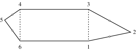
Figure 21: A hexagon that folds by gluing together vertices $\{v_{1},v_{2},v_{3}\}$ to form one node, and $\{v_{4},v_{5},v_{6}\}$ to form the other. Note the angle sum at the former is $\pi/2+\pi/2$ from the right angles at $v_{1}$ and $v_{3}$, and $\pi$ from $\triangle(v_{1},v_{2},v_{3})$, for a total of $2\pi$. The four fold vertices are marked.

Theorem 5.14

A convex polygon $P$ of $n$ vertices folds to at most $O(n^{3})$ different gluing trees.

Proof: Theorem 4.6 limits the combinatorial possibilities to trees with four or fewer leaves. We have settled each case for ${\lambda}\leq 4$ earlier:

${\lambda}=4$

Lemma 5.13: $O(1)$.

${\lambda}=3$

Lemma 5.5: $O(n^{4})$.

${\lambda}=2$

Lemma 5.4: $O(n^{2})$.

We now improve the ${\lambda}=3$ case to $O(n^{3})$ for convex polygons. We can tighten the $O(n^{4})$ bound with the following two observations:

1. The two internal angles at the two vertices glued at a type-vve node must sum to no more than $\pi$.

2. A convex polygon cannot have too many vertices with small angles.

To quantify the second observation, define the turn angle $\tau_{i}$ at a vertex $v_{i}$ with internal angle ${\alpha}_{i}$ to be $\tau_{i}=\pi-{\alpha}_{i}$. For any polyon, we must have $\sum_{i}=2\pi$. For a convex polygon, $\tau_{i}>0$. Now suppose $v_{i}$ and $v_{j}$ glue at a type-vve node. Then ${\alpha}_{i}+{\alpha}_{j}\leq\pi$, and so $\tau_{i}+\tau_{j}\geq\pi$. Thus two distinct vv-gluings, involving four different vertices, already consume the available $2\pi$ turn angle of the polygon. Call two pairs of vertices disjoint if all four vertices are different. The turn angle bound implies that any polygon can have at most two disjoint pairs of vertices glued to a type-vve node. We now show that this implies a $O(n)$ bound on the number of type-vve nodes.

Construct a bipartite graph $H$ with $n$ nodes for the first vertex and $n$ nodes for the second vertex of vv-gluings. Let $(v_{i},v_{j})$ and $(v_{k},v_{l})$ be disjoint pairs in vv-gluings, as depicted in Fig. 16(b). Then because there cannot be another pair disjoint from either of these, every other pair must be incident to one of the four vertices $v_{i},v_{j},v_{k},v_{l}$. This limits $H$ to at most $4n$ edges (and even this bound is loose, for this permits as many as four disjoint pairs, as is evident in the figure).

Thus there are at most $O(n)$ type-vve nodes. Repeating the argument that a vv-gluing determines one leg of the ‘Y’ and Lemma 5.4 bounds the remaining path to $O(n^{2})$ possibilities, leads to the claimed $O(n^{3})$ bound. $\Box$

We leave open the question of whether this bound is tight.

It is straightforward to list all possible gluing trees for a given convex polygon with an $O(n^{3}\log n)$ time algorithm. We have implemented such an algorithm, with, however, less than maximally efficient data structures.

6 Counting Foldings: Noncongruent Polytopes

We have so far been counting the number of different ways to fold up a given polygon, but have not addressed the question of whether all these foldings produce distinct polytopes. There are several notions of what constitutes distinctness. One natural definition relies on the combinatorial structure of the polytope, as explored by Shephard [She75]. We will have little to say on this topic here. Instead, we will focus on counting noncongruent polytopes.

We have already established in Lemma 5.7 that any rectangle can fold to an uncountably infinite number of noncongruent tetrahedra. We extend this result in this section to the “obvious” fact that any convex polygon folds (via perimeter-halving) to an uncountably infinite number of noncongruent polytopes. Despite the naturalness of this claim, our inability to determine the 3D structure of the polytope guaranteed by an Aleksandrov gluing makes our proof less than satisfactory. In the absence of any 3D information, we concentrate instead on the pattern of geodesics between vertices, for of course two congruent polytopes have the exact same set of geodesics.

Lemma 6.1

A polytope $Q$ resulting from a perimeter-halving fold of polygon $P$ has a countable number of geodesics between any pair of vertices.

Proof: Let $x$ and $y$ be the fold vertices produced by the perimeter-halving (as in Fig. 1). We will assign each geodesic a unique integer, which establishes that there are only a countable number of them. The integers are based on a “layout” of the surface of $Q$ in the plane. Fix $P$ in the plane, and designate it as level-$0$ of the layout. Around ${\partial P}$ layout $2n$ copies of $P$ (where $P$ has $n$ vertices) corresponding to the perimeter gluing. These are level-$1$ $P$ copies of the layout. This level is illustrated in Fig. 22. For example, because edge $e_{4}=v_{4}v_{5}$ of ${\partial P}$ is glued into the edge $e_{1}=v_{1}v_{2}$ by the perimeter halving, a level-$1$ copy of $P$ is placed exterior to $e_{4}$ arranged so that the glued portions of $e_{4}$ and $e_{1}$ match. There are $2n$ level-$1$ copies of $P$ because the $n$ vertices around ${\partial P}$ are interspersed by a reversed sequence of the same $n$ vertices.

Continuing the construction, level-$i$ of the layout is formed by surrounding each level-$(i{-}1)$ copy of $P$ with $2n$ additional copies. Give these copies a “sequence number” $j=1,\dots,2n$. Now every copy of $P$ at level-$i$ in the layout may be assigned a unique integer by listing the sequence numbers for each level $0,\ldots,i$ and interpreting it as a base-$2n$ number.

It is clear from the layout construction that any geodesic on $Q$ “unrolls” to a straightline in the layout. Because we can number the copies of $P$, we can number the geodesics between any given pair of vertices. Therefore the number of geodesics is denumerable. $\Box$

Although this proof is specialized to polytopes formed from perimeter halving, it would not be difficult to extend it to all polytopes formed by gluings including a “rolling” fold-point.

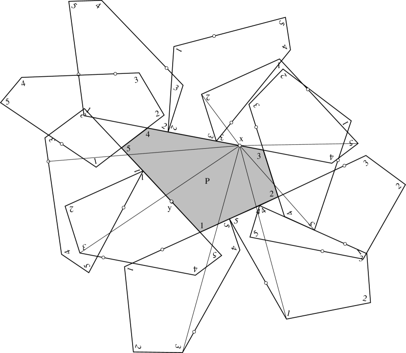
Figure 22: Layout of a perimeter-halving folding of a pentagon. Several geodesics are shown from $x$ to level-$1$ vertices.

Theorem 6.2

Any convex polygon $P$ folds, via perimeter halving, to a uncountably infinite number of noncongruent polytopes.

Proof: Select $x$, a fold point for perimeter halving, interior to an edge $e_{i}=v_{i}v_{i+1}$ of $P$. The segment $xv_{i}\subset{\partial P}$ in level-$0$ of the layout used in the previous lemma corresponds to a geodesic on $Q_{x}$. Now let $x$ vary within some neighborhood $N\subset e_{i}$; let $x^{\prime}\neq x$ be a point in $N$. The segment $x^{\prime}v_{i}$ corresponds to a geodesic on $Q_{x^{\prime}}$ of a different length. We use this fact to establish our claim.

Let ${\cal Q}=\{Q_{x^{\prime}}\;:\;x^{\prime}\in N\}$ be the set of all the polytopes produced as $x$ varies over the neighborhood. Assume, for the purposes of contradiction, that the number of distinct, noncongruent polytopes in $\cal Q$ is denumerable: $Q_{1},Q_{2},\ldots$. By Lemma 6.1, each has a countable number of geodesics: a pair of numbers suffice to uniquely identify them. Thus the total number of distinct lengths of geodesics represented by all these polytopes is denumerable. But this contradicts the nondenumerable number of lengths of segments $|x^{\prime}v_{i}|$ for $x^{\prime}\in N$. Therefore the number of noncongruent polytopes in $\cal Q$ is nondenumerable. $\Box$

Although this theorem establishes the result even for regular polygons, there is much more to say about the structure of the polytopes that can be folded from regular polygons. We explore this in Section 9.

7 Counting Unfoldings: Cut Trees

In this section we explore unfolding from the point of view of cut trees. The general situation is that we are given one polytope $Q$ of $n$ vertices, and we would like to know how many different ways it can be cut and unfolded to a polygon. We start with some straightforward observations before proving enumeration bounds.

First, every polytope admits at least the $n$ cut trees provided by the star unfolding [AO92], one with each vertex as source. So in particular, every polytope unfolds to at least one polygon. (As we mentioned in the Introduction, the corresponding question for edge-unfoldings remains open.)

Second, because we permit arbitary polygonal paths between the nodes of a cut tree (Section 3), there is no upper bound on the number of polygon vertices in potential unfoldings of a given polytope. This might lead one to wonder if any polygon (of the appropriate area) can be unfolded from a given polytope. The answer is no, as is easily established by this lemma.

Lemma 7.1

Every polygon $P$ cut from $Q$ must have at least two vertices whose interior angles are of the form $2\pi-{\gamma}_{i}$ for some $i=1,\ldots,n$, where ${\gamma}_{i}$ are the curvatures of the vertices of $Q$.

Proof: Let the $n$ vertices of $Q$ have curvatures ${\gamma}_{i}$, $i=1,\ldots,n$. The cut tree $T_{C}$ must have at least two leaves, and by Lemma 3.1 these leaves must be vertices of $Q$. Say they coincide with the vertices of curvatures ${\gamma}_{1}$ and ${\gamma}_{2}$. Then any polygon $P$ that unfolds from $T_{C}$ must have two vertices with interior angles $2\pi-{\gamma}_{1}$ and $2\pi-{\gamma}_{2}$. $\Box$

So let $P$ be a polygon with no interior angle equal to $2\pi-{\gamma}_{i}$ for $i=1,\ldots,n$. Then $P$ cannot be cut from $Q$.

7.1 Lower Bound: Exponential Number of Unfoldings

In this section we provide an exponential lower bound.

Theorem 7.2

There is a polytope $Q$ of $n$ vertices that may be cut open with exponentially many ($2^{\Omega(n)}$) combinatorially distinct cut trees, which unfold to exponentially many geometrically distinct simple polygons.

Proof: $Q$ is a truncated cone, as illustrated in Fig. 23:

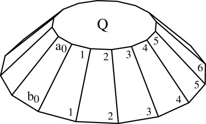
Figure 23: Polytope $Q$.

the hull of two regular $n$-gons of different radii, lying in parallel planes and similarly oriented. We call this the volcano example. We require that $n$ be even; in the figure, $n=16$. Label the vertices on the top face $a_{0},\ldots,a_{n-1}$ and $b_{0},\ldots,b_{n-1}$ correspondingly on the bottom face. The “base” cut tree, which we notate as $T_{0000000}$, unfolds $Q$ as shown in Fig. 25. $T_{0000000}$ consists of a path on the top face $(a_{0},a_{1},\ldots,a_{n-1})$ supplemented by arcs $(a_{i},b_{i})$ for all $i=0,\ldots,n-1$. The polygon $P$ produced consists of the base face, $n$ attached trapezoids $(b_{i},b_{i+1},a_{i+1},a_{i})$, with the top face attached to $a_{n-1}a_{0}$.

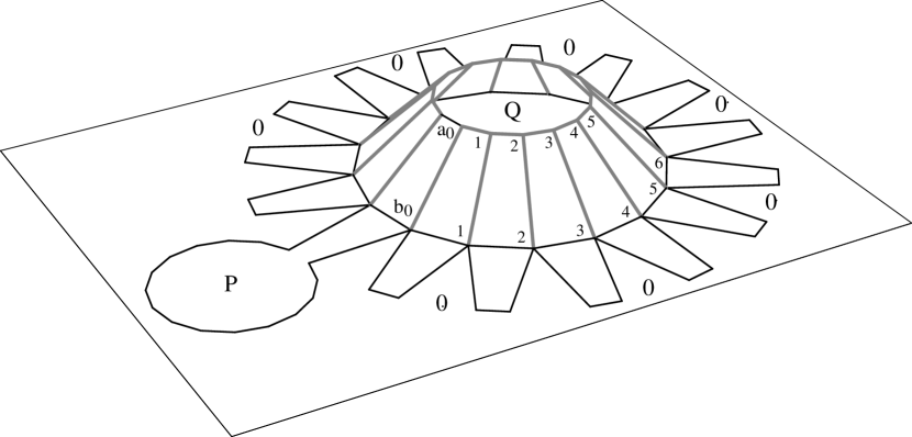
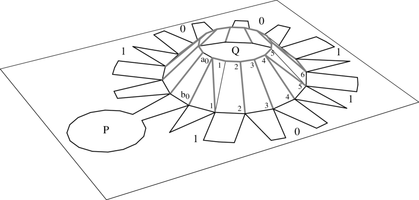
Figure 24: Unfolding via shaded cut tree $T_{0000000}$.

Figure 25: Unfolding via shaded cut tree $T_{1001101}$.

Define a cut tree $T_{m_{(n-1)/2}\cdots m_{2}m_{1}m_{0}}$, where $m_{i}$ are the digits of a binary number of $n/2-1$ bits, as an alteration of the base tree $T_{0\cdots 0}$ as follows. If $m_{i}=1$, then the arc $(a_{2i+1},b_{2i+1})$ is deleted and replaced by $(a_{2i},b_{2i+1})$. If $m_{i}=0$, then the arc $(a_{2i+1},b_{2i+1})$ is used as in $T_{0\cdots 0}$. Thus the cut tree $T_{1001101}$ shown in Fig. 25 replaces $(a_{1},b_{1})$ with $(a_{0},b_{1})$ because $m_{0}=1$, $(a_{5},b_{5})$ with $(a_{4},b_{5})$ because $m_{2}=1$, and so on.

There are $2^{n/2-1}=2^{\Omega(n)}$ cut trees.

It is clear by construction that all these cut trees lead to simple polygon unfoldings. It only remains to argue that each leads to a distinct polygon, not congruent to any other. This is not strictly true for $Q$ as defined, for any bit pattern leads to a $P$ that is congruent (by reflection) to the polygon obtained from the reverse of the bit pattern. However, it is a simple matter to introduce some asymmetry, by, for example, lengthening edge $a_{n-1}a_{0}$ slightly. Then all cut trees lead to distinct polygons. $\Box$

A simpler example is a drum, the convex hull of two regular polygons in parallel planes. Because some of the unfoldings used in the above proof overlap, there is a bit more argument needed to establish the exponential lower bound.

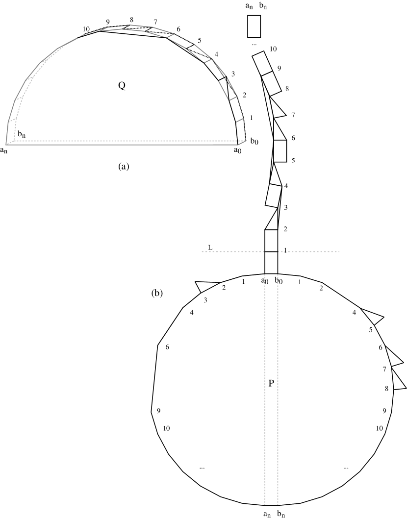
Figure 26: (a) Polytope $Q$, cut tree $T_{\cdots 0022020100}$. The $a$-path is shown solid, the $b$-path dashed. (b) Unfolding to polygon $P$. $L$ strictly separates the head from the tail.

Even restricting the cut tree to a path permits an exponential number of unfoldings:

Theorem 7.3

There is a polytope $Q$ of $n$ vertices that may be cut open with exponentially many ($2^{\Omega(n)}$) combinatorially distinct cut trees, all of which are paths, which unfold to exponentially many geometrically distinct simple polygons.

Proof: $Q$ is formed by pasting two halves of a regular $2n$-gon together to form a semicircle approximation with some small thickness $w>0$. Label the vertices on the front face $a_{0},\ldots,a_{n}$ and $b_{0},\ldots,b_{n}$ correspondingly on the back face, as illustrated in Fig. 26(a). Let ${\alpha}=2\pi/n$ be the turn angle at each vertex $a_{i}$ (and at $b_{i}$), i.e., the angle ${\alpha}=\pi-\angle(a_{i-1},a_{i},a_{i+1})$. (In the figure, ${\alpha}=\pi/32\approx 11^{\circ}$.) We specify a series of cut trees $T_{m}$, where $m$ is an $n$-digit base-$3$ integer $m_{n}\cdots m_{2}m_{1}$, with the following interpretation. $T_{0\cdots 00}$ is the “base” cut tree on which all others are variations:

$$T_{0\cdots 00}=(a_{0},a_{1},\ldots,a_{n},b_{n},b_{n-1},\ldots,b_{1},b_{0})$$ (11)

Note that $T_{0\cdots 00}$ is a path, as are all the $T_{m}$. We call the half of the path on the front face the $a$-path, and that on the back the $b$-path. The unfolding $P$ determined by $T_{0\cdots 00}$ is a regular $2n$-gon, fattened by a strip $(a_{0},b_{0},b_{n},a_{n})$ of width $w$ down its middle, with a “tail” of $n$ rectangles attached to edge $a_{0}b_{0}$. If $|a_{i}a_{i+1}|=h$, then each rectangle is $w\times h$.

In cut tree $T_{m_{n}\cdots m_{2}m_{1}}$ the index $m_{i}$ is $1$ if the $a$-path deviates to touch $b_{i}$ on the back face via the path $(\ldots,a_{i-1},b_{i},a_{i},a_{i+1},\ldots)$, and the index $m_{i}$ is $2$ if the $b$-path similarly deviates to include $a_{i}$ on the front face via the path $(\ldots,b_{i-1},a_{i},b_{i},b_{i+1},\ldots)$. In both cases, the opposite path skips the vertex deviated to: if $m_{i}=1$, the $b$-path skips $b_{i}$ by shortcutting on the back face, and if $m_{i}=2$, the $a$-path skips $a_{i}$ by shortcutting on the front face. Fig. 26(a) illustrates $T_{m_{n}\cdots 0022020100}$, with $a$-path

$$(a_{0},a_{1},a_{2},b_{3},a_{3},a_{4},a_{6},a_{9},a_{10},\ldots,a_{n})$$ (12)

and $b$-path

$$(b_{0},b_{1},b_{2},b_{4},a_{5},b_{5},b_{6},a_{7},b_{7},a_{8},b_{8},b_{9},b_{10},\ldots,b_{n})$$ (13)

Note that when $m_{i}\neq 0$, the rectangle bounded between $a_{i-1}b_{i-1}$ and $a_{i}b_{i}$ is crossed by an $ab$-diagonal. We insist that $m_{1}=0$, so that the cut tree starts with an uncrossed rectangle $(a_{0},b_{0},b_{1},a_{1})$. Finally, the edge $a_{n}b_{n}$ is included in $T_{m}$, so that it is a path from $a_{0}$ to $a_{n}$ to $b_{n}$ and returning to $b_{0}$. The digits $m_{n}\cdots m_{2}$ are each free to be any one of $\{0,1,2\}$. Thus there are an exponential number of combinatorially distinct $T_{m}$: $3^{n-1}$. We return below to the issue of how many of these lead to geometrically distinct unfoldings.

It should be clear by construction that $T_{m}$ spans the vertices. To show that it is a tree, we need to argue that it is non-self-intersecting. This is again clear by construction, for each nonzero $m_{i}$ uses a diagonal in the rectangle prior to $a_{i}b_{i}$, and because $m_{i}$ has only one value, no such rectangle has both diagonals used. Together with the shortcutting that prevents the $a$- and $b$-paths from touching the same vertex, it follows that $T_{m}$ is indeed a tree; so it is a legitimate cut tree. Thus it unfolds to a single piece. It only remains to show that this unfolding is a simple polygon, i.e., it avoids overlap.

This is obvious for $T_{0\cdots 00}$, as mentioned previously. For general $T_{m}$, consider the layout of the unfolding $P$ that places $a_{0}b_{0}$ horizontally, as in Fig. 26(b). Let $L$ be the horizontal line through $a_{1}b_{1}$; this segment is necessarily horizontal because we stipulated that $m_{1}=0$. We will argue that $L$ strictly separates the tail of $P$ (the portion attached above $a_{1}b_{1}$) from its body (the portion attached below $a_{1}b_{1}$).

First, it is clear that the body unfolds without overlap. For it is simply truncations (due to path shortcuttings) of halves of a regular polygon glued to either side of the rectangle $(a_{0},b_{0},b_{n},a_{n})$, with attached triangle “spikes” for each nonzero $m_{i}$. None of these spikes can overlap, even when adjacent, for their length-$w$ edge juts out orthogonal to their length-$h$ edge glued to the body (see the body image of $b_{7}$ in Fig. 26(b)).

The tail consists of $h\times w$ rectangles, or half-rectangles, glued end-to-end, with turns to the right by ${\alpha}$ for every $m_{i}=1$ digit, and turns to the left by ${\alpha}$ for every $m_{i}=2$ digit. Thus, $T_{\cdots 0022020100}$ in (b) of the figure turns right once and left three times. Because there are at most $n-1$ nonzero digits, the tail can turn at most $n-1$ times. Because ${\alpha}$ is the turn angle of a regular $2n$-gon, it takes $n$ turns of ${\alpha}$ to turn a full $\pi$. Thus the tail turns strictly less than $\pi$, and so cannot return to line $L$. Thus the tail remains strictly above $L$. Choosing $w<h$ guarantees that no body spike protrudes vertically as much as $h$ above $a_{0}b_{0}$; so the body remains strictly below $L$.

It remains to argue that the tail does not self-intersect. But this follows from the same turn argument above. By construction, there are no local overlaps between two adjacent tail rectangles or half-rectangles. Thus the only overlap conceivable would result from the tail curling back to overlap itself. Choosing $w\ll h$ makes the tail essentially a series of segments of length $h$, with attached pieces of the regular polygon clipped by shortcutting. For the tail segments to curl back and overlap would require a total turn by at least $\pi$, contradicting the bound on the sum of ${\alpha}$’s.

Finally, we turn to the question of how many of the $3^{n-1}$ combinatorially distinct $T_{m}$ lead to geometrically distinct (noncongruent) $P$. Let $x$ and $y$ be two base-$3$ numbers, and let $S(x)$ be the base-$3$ number obtained by changing each $1$-digit in $x$ to a $2$, and each $2$-digit in $x$ to a $1$. (For example, $S(1021)=2012$.) Then if $S(x)=y$, $T_{x}$ and $T_{y}$ lead to congruent $P$, in that $P_{y}$ is the reflection of $P_{x}$ about a vertical line (in the layout used above).

Although we could easily ensure noncongruency for all $T_{m}$ by altering $Q$ to be less symmetric, we opt here for a counting argument. Let $x$ be a base-$3$ number. Define $B(x)$ to be the binary number obtained by changing each $2$-digit in $x$ to a $1$. (For example, $B(2012)=1011$.) Now it should be clear that for any two base-$3$ numbers $x$ and $y$, if $B(x)\neq B(y)$, then $P_{x}$ is noncongruent to $P_{y}$. For then the pattern of spikes on the body are different in $P_{x}$ and $P_{y}$. Thus, among the $3^{n-1}$ combinatorially distinct $P$, there are at least $2^{n-1}$ geometrically distinct $P$. $\Box$

7.2 Lower Bound: Convex Unfoldings

It seems possible that the exponential lower bound holds even in the case of convex unfoldings, via an example similar to that used in Fig. 26.

Conjecture 7.1

There is a polytope with an exponential number of convex unfoldings.

This represents the only ‘?’ in Table 1.

7.3 Upper Bound

Theorem 7.4

The maximum number of edge-unfolding cut trees of a polytope of $n$ vertices is $2^{O(n)}$, and the maximum number of arbitary cut trees $2^{O(n^{2})}$.

Proof: For edge unfoldings, the bound depends on the number of spanning trees of a polytope graph. We may obtain a bound here as follows. First, triangulating a planar graph only increases the number of spanning trees, so we may restrict attention to triangulated planar graphs. Second, it is well known that the number of spanning trees of a connected planar graph is the same as the number of spanning trees of its dual. So we focus just on $3$-regular (cubic) planar graphs. Finally, a result of McKay [McK83] proves an upper bound of $O((16/3)^{n}/n)$ on the number of spanning trees for cubic graphs. This bound is $2^{O(n)}$.

For arbitrary cut trees, the underlying graph might conceivably have a quadratic number of edges, which leads to the bound $2^{O(n^{2})}$. (Note that our definition of cut tree in Section 3.1 would not count different polygonal paths between two vertices as distinct arcs of $T_{C}$.) $\Box$

8 Counting Unfoldings: Noncongruent Polygons

We have already seen in Theorem 7.2 that one polytope can have an exponential number of noncongruent polygon unfoldings. In fact the possibilities range from $0$ to $\infty$, even for convex unfoldings, as this simple counterpart of Theorem 6.2 shows:

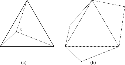
Figure 27: Unfolding a flat triangle (a) to a convex polygon (b).

Theorem 8.1

Although some polytopes unfold to a nondenumerable number of noncongruent convex polygons, others have only a finite number of convex unfoldings.

Proof: For the former claim, consider a doubly-covered equilateral triangle. Choose any point $x$ interior to the top face, as shown in Fig. 27(a). This leads to a ‘Y’ cut tree that unfolds to a convex polygon (b) for every choice of $x$. All these polygons have different angles, and so are noncongruent.

The second claim of the theorem is trivially satisfied by polytopes with zero convex unfoldings. To establish it for a polytope that has at least one convex unfolding is more difficult, and we only sketch a construction. Consider the doubly-covered trapezoid shown in Fig. 28. It has just two sharp vertices, $v_{1}$ and $v_{4}$, and so, by Theorem 4.6, the cut tree must be a path connecting those vertices. The path $(v_{1},v_{2},v_{3},v_{4})$ unfolds to a convex polygon. Now consider a geodesic that starts with the segment $v_{1}v_{3}$ as illustrated. As in the proof of Lemma 4.5, this geodesic will either hit $v_{4}$ directly, in which case it is not a valid cut tree because $v_{2}$ is not spanned, or it spirals around the trapezoid and self-crosses. We will not prove this claim. $\Box$

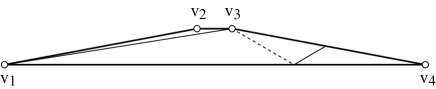
Figure 28: A geodesic on a trapezoid from $v_{1}$ through $v_{3}$.

9 Folding Regular Polygons

In this section we study folding regular polygons of $n$ vertices. Because all polygon vertices have the same interior angle ${\theta}=(n-2)\pi/n$, only a limited variety of different polytope vertex curvatures may be created. We find, not surprisingly, that this leads to a limited set of possibilities: in general, only one “class” of nonflat polytopes can be produced. This is established in Lemma 9.2.

Let ${\alpha}_{k}$, $k\geq 1$, be the curvature at a polytope vertex formed by gluing $k$ $P$-angles of ${\theta}$ together, and ${\beta}_{k}$, $k\geq 0$, be the curvature at a vertex formed by gluing $k$ angles to a point interior to an edge of ${\partial P}$. The next lemma details the possible ${\alpha}_{k}$ and ${\beta}_{k}$ values achievable.

Throughout this section we will find that the situation is more uniform for $n>6$ than it is for small $n$.

Lemma 9.1

For $n>6$, only four vertex curvatures can be obtained by folding a regular $n$-gon $P$; for $n\leq 6$, additional curvature values are possible. More precisely, for all $n$, these four curvature values are always achievable:

• ${\alpha}_{1}=\pi(1+2/n)$.

• ${\alpha}_{2}=\pi(4/n)$.

• ${\beta}_{0}=\pi$.

• ${\beta}_{1}=\pi(2/n)$.

The additional values possible for $n\leq 6$ are detailed in Tables 2 and  3.

Proof:

1. ${\alpha}_{1}=2\pi-{\theta}=2\pi-(n-2)\pi/n=\pi(1+2/n)$. This vertex is a leaf of the gluing/cut tree. We call this a zipped vertex, for ${\partial P}$ is “zipped shut” at the vertex.

2. ${\alpha}_{2}=2\pi-2{\theta}=2\pi-2(n-2)\pi/n=\pi(4/n)$. This vertex is a degree-$1$ node of the gluing tree.

3. ${\beta}_{0}=\pi$. This is a fold vertex, when nothing is glued to an edge of ${\partial P}$, and therefore a leaf of the gluing tree.

4. ${\beta}_{1}=2\pi-[\pi+{\theta}]=2\pi-[\pi+(n-2)\pi/n]=\pi(2/n)$. This is a degree-$1$ node of the gluing tree.

The additional possibilities for $n\leq 6$ are as follows. ${\alpha}_{3}$ is possible for all $n\leq 6$; ${\alpha}_{4}$ is possible only for $n=4$; and no other ${\alpha}_{k}$ is possible. See Table 2.

For $n=3$, ${\beta}_{2},{\beta}_{3}$, and for $n=4$, ${\beta}_{2}$, are all possible. See Table 3.

Explicit computation shows that all higher values of $k$ lead to nonconvex vertices, whose total face angle exceeds $2\pi$ and so which have negative curvature. $\Box$

${\alpha}_{k}$	$k$
	1	2	3	4
3	$\frac{5}{3}$	$\frac{4}{3}$	$1$
4	$\frac{3}{2}$	$1$	$\frac{1}{2}$	$0$
5	$\frac{7}{5}$	$\frac{4}{5}$	$\frac{1}{5}$
6	$\frac{4}{3}$	$\frac{2}{3}$	$0$
$n$	$1+\frac{2}{n}$	$\frac{4}{n}$

Table 2: Possible ${\alpha}_{k}$ curvature values, in units of $\pi$.

${\beta}_{k}$	$k$
	0	1	2	3
3	$1$	$\frac{2}{3}$	$\frac{1}{3}$	$0$
4	$1$	$\frac{1}{2}$	$0$
$n$	$1$	$\frac{2}{n}$

Table 3: Possible ${\beta}_{k}$ curvature values, in units of $\pi$.

Let $a_{i}$ and $b_{i}$ be the number of polytope vertices of curvature ${\alpha}_{i}$ and ${\beta}_{i}$ respectively, formed by folding a regular $n$-gon $P$. Of course $a_{i}$ and $b_{i}$ are nonnegative integers, but there are additional significant restrictions imposed by the requirement that the total curvature be $4\pi$:

$$\sum_{i=1}a_{i}{\alpha}_{i}+\sum_{i=0}b_{i}{\beta}_{i}=4\pi\;.$$ (14)

We now explore the implications of this constraint, separately for $n>6$ and for $n\leq 6$. Note that our notation implies that

$$\sum_{i=1}a_{i}i+\sum_{i=0}b_{i}i=n\;,$$ (15)

because the subscripts on ${\alpha}$ and ${\beta}$ indicate the number of vertices involved in the gluing.

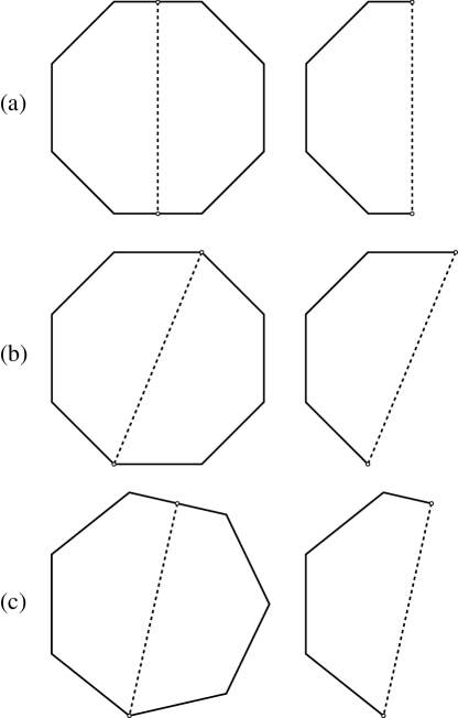
Figure 29: (a,b) Flat foldings of an $n$-gon, $n$ even ($n=8$). (c) Flat folding of an $n$-gon, $n$ odd ($n=7$).

Now we prove that perimeter-halving is the only possible kind of folding for $n>6$.

Lemma 9.2

For all $n\geq 3$, regular $n$-gons fold via perimeter-halving, using path gluing trees, to two classes of polytopes:

1. A continuum of “pita” polytopes of $n+2$ vertices.

2. One or two flat, “half-$n$-gons”:

   1. $n$ even: Two flat polytopes, of $\frac{n}{2}+2$ and $\frac{n}{2}+1$ vertices.

   2. $n$ odd: One flat polytope, of $\frac{n+1}{2}+1$ vertices.

For $n>6$, these are the only foldings possible of a regular $n$-gon.

Proof: A perimeter-halving fold produces a path gluing tree. This has two leaves and all other nodes internal. From Lemma 9.1, the only two curvatures can be leaves: $\{{\alpha}_{1},{\beta}_{0}\}$; and only two can be degree-$1$ nodes: $\{{\alpha}_{2},{\beta}_{1}\}$. Moreover, these are the only curvatures possible for $n>6$. Thus Eq. (14) reduces to

$$a_{1}{\alpha}_{1}+a_{2}{\alpha}_{2}+b_{0}{\beta}_{0}+b_{1}{\beta}_{1}=4\pi\;.$$ (16)

Substituting the curvature values from Lemma 9.1 and solving for $n$ yields

$$n=\frac{2(a_{1}+2a_{2}+b_{1})}{4-(a_{1}+b_{0})}\;$$ (17)

Because only ${\alpha}_{1}$ and ${\beta}_{0}$ are leaf vertex curvatures, we must have $a_{1}+b_{0}\geq 2$. The requirement that the denominator of Eq. (17) be positive yields $a_{1}+b_{0}<4$. Therefore we know that $a_{1}+b_{0}\in\{2,3\}$. We now show that the case $a_{1}+b_{0}=3$ is not possible when $n>6$.

As both $a_{1}$ and $b_{0}$ count leaves, a tree formed with $a_{1}+b_{0}=3$ must have at least three leaves. By Theorem 4.6, because $n\neq 4$, it cannot have more than three leaves. So it has exactly three leaves, and has the combinatorial structure of a ‘Y’. The interior node must be formed by gluing three distinct points of ${\partial P}$ together (by Lemma 3.1(4)). This corresponds to curvatures ${\alpha}_{k}$, $k\geq 3$, or ${\beta}_{k}$, $k\geq 2$. But Lemma 9.1 shows that none of these are possible for $n>6$. (Note, for later reference, that for $n\leq 6$, these possibilities will need consideration.)

Therefore we must have $a_{1}+b_{0}=2$. Therefore the gluing tree must be a path for $n>6$, and the folding must be a perimeter-halving folding. We now explore the three possible solutions to $a_{1}+b_{0}=2$.

Case $a_{1}=0$, $b_{0}=2$.

The two leaves are both folds at interior points of edges of ${\partial P}$, a perimeter-halving folding similar to that previously illustrated in Fig. 1. If neither fold point $x$ and $y$ is the midpoint of its edge, then no pair of vertices glue together, so $a_{2}=0$ and therefore $b_{1}=n$. This produces a continuum of polytopes $Q_{x}$ of $n+2$ vertices. We call these pita polytopes (Fig. 32), and will study them in Section 9.1 below.

Suppose one fold point $x$ is at an edge midpoint. If $n$ is even, then $y$ is also at a midpoint, and $P$’s vertices are glued in pairs. Therefore $a_{2}=n/2$ and $b_{1}=0$. The polytope is a flat half-$n$-gon of $n/2+2$ vertices. See Fig. 29(a). If $n$ is odd, then $y$ must be at a vertex. This means that $a_{1}\neq 0$, and this case does not apply.

Case $a_{1}=2$, $b_{0}=0$.

Both leaves are at vertices, and so $n$ must be even. All other vertices are glued in pairs, so $a_{2}=(n-2)/2$ and $b_{1}=0$. The folding produces a flat half-$n$-gon of $n/2+1$ vertices. See Fig. 29(b).

Case $a_{1}=1$, $b_{0}=1$.

One vertex is zipped to a leaf; half the perimeter around is a fold vertex. This implies that $n$ is odd. All other vertices are glued in pairs, so $a_{2}=(n-1)/2$ and $b_{1}=0$. The folding produces a flat half-$n$-gon of $(n-1)/2+2$ vertices. See Fig. 29(c).

The details derived above are gathered into Table 4, and the flat foldings illustrated in Fig. 29. $\Box$

$n$	$a_{1}$	$b_{0}$	$a_{2}$	$b_{1}$	$N$	description
any	$0$	$2$	$0$	$n$	$n+2$	pita polyhedra
even	$0$	$2$	$\frac{n}{2}$	$0$	$\frac{n}{2}+2$	flat half-$n$-gon
even	$2$	$0$	$\frac{n}{2}-1$	$0$	$\frac{n}{2}+1$	flat half-$n$-gon
odd	$1$	$1$	$\frac{n-1}{2}$	$0$	$\frac{n+1}{2}+1$	flat half-$n$-gon

Table 4: Fold cases for regular $n$-gons, $n>6$. $N$ is the number of polytope vertices.

Lemma 9.3

For $n\leq 6$, regular polygons fold to additional polytopes (beyond those listed in Lemma 9.2) as detailed in Table 5.

Proof: Lemma 3.1 limits the possible nonpath cut trees to ‘Y’, ‘+’, and ‘I’. We first argue that ‘I’ is only possible for $n=6$. The two interior nodes of the tree must have curvatures in $\{{\alpha}_{3},{\beta}_{2}\}$. For $n=3$, there are not enough vertices to make these nodes. For $n=4$, there are enough vertices to make two ${\beta}_{2}$ nodes, but this then forces the ‘+’ structure, i.e., the interior edge of the ‘I’ has length zero. For $n=5$ and $n=6$, ${\beta}_{2}$ is not possible. For $n=5$, there are not enough vertices to make two ${\alpha}_{3}$ vertices. And finally, for $n=6$, there are enough vertices, and the folding produces a flat rectangle.

Thus only ‘Y’ and ‘+’ are possible. The ‘+’ can only be realized in two ways: by gluing four vertices together, which is only possible for $n=4$ (see ${\alpha}_{4}$ column in Table 2), and by gluing three vertices to an edge, which is only possible for $n=3$ (see ${\beta}_{3}$ column in Table 3).

There are a number of ways to realize ‘Y’-trees. The constraint that the curvature add to $4\pi$, Eq. (14), together with the discrete set of possible curvatures in Tables 2 and 3, lead to the possibilities listed in Table 5. (The second line of the table was previously illustrated in Fig. 3.) $\Box$

$n$	Tree	Gluing Description	Curvatures	$N$	Polytope Description
$3$	‘Y’	3 v	${\alpha}_{3}+3{\beta}_{0}$	$4$	tetrahedron
$3$	‘Y’	2 v + inc e	${\alpha}_{1}+2{\beta}_{0}+{\beta}_{2}$	$4$	$\infty$ tetrahedra
$3$	‘Y’	2 v + adj e	$3{\beta}_{0}+3{\beta}_{1}$	$4$	$\infty$ $5$v polytopes
$3$	‘+’	3 v + e	$4{\beta}_{0}+{\beta}_{3}$	$4$	$\infty$ tetrahedra
$4$	‘Y’	3 v	${\alpha}_{1}+2{\beta}_{0}+{\alpha}_{3}$	$4$	tetrahedron
$4$	‘Y’	2 adj v + opp e	$3{\beta}_{0}+2{\beta}_{1}+{\beta}_{2}$	$5$	$\infty$ $5$v polytopes
$4$	‘Y’	2 adj v + inc e	$4{\beta}_{0}+2{\beta}_{2}$	$4$	$\infty$ tetrahedra
$4$	‘Y’	2 adj v + adj e	$3{\beta}_{0}+2{\beta}_{1}+{\beta}_{2}$	$5$	$\infty$ $5$v polytopes
$4$	‘Y’	2 opp v	$2{\beta}_{0}+2{\beta}_{1}+{\beta}_{2}$	$4$	$\infty$ tetrahedra
$4$	‘+’	4 v	${\alpha}_{4}+4{\beta}_{0}$	$4$	flat square
$5$	‘Y’	2 adj v + 1 opp v	$2{\alpha}_{1}+{\alpha}_{3}+{\beta}_{0}$	$4$	tetrahedron
$5$	‘Y’	3 adj v	${\alpha}_{2}+{\alpha}_{3}+3{\beta}_{0}$	$5$	$5$v polytope
$6$	‘Y’	3 alt v	$3{\alpha}_{1}+{\alpha}_{3}$	$3$	flat triangle
$6$	‘Y’	3 adj v	${\alpha}_{1}+{\alpha}_{2}+{\alpha}_{3}+2{\beta}_{0}$	$4$	tetrahedron
$6$	‘Y’	2 adj v + v	${\alpha}_{1}+{\alpha}_{2}+{\alpha}_{3}+2{\beta}_{0}$	$4$	tetrahedron
$6$	‘I’	3 adj v, 3 adj v	$2{\alpha}_{3}+4{\beta}_{0}$	$4$	flat rectangle

Table 5: Additional fold possibilities for regular $n$-gons, $n\leq 6$. $N$ is the number of polytope vertices. Notation in Gluing Description column: v = vertex, e = edge, adj = adjacent, alt = alternate, opp = opposite, inc = included. In the Polytope Description column: $\infty$ = continuum of, $5$v polytope = $5$-vertex polytope. Each entry of the Curvatures column satisfies Eqs. (14) and (15).

If we treat the $n$ vertices of a regular $n$-gon as assigned the same label (as seems appropriate), Lemmas 9.2 and 9.3 together show that there are only $O(1)$ ways to fold up a regular polygon, justifying the entry in Table 1. If we label the vertices with distinct labels, then there are $O(n)$ foldings.

9.1 Pita Polytopes

We define a pita polytope as one obtained by a perimeter-halving folding of a regular polygon at a point on an edge that is not a midpoint, as per the first line of Table 4. Let the regular $n$-gon $P$ have unit edge length, and let the fold points $x$ be distance $a$ from $v_{0}$ along edge $v_{0}v_{1}$. Let $b=1-2a$. Call the point along ${\partial P}$ to which $v_{i}$ glues $v^{\prime}_{i}$. See Fig. 30 for an example with $n=12$. We will use this example throughout the section.

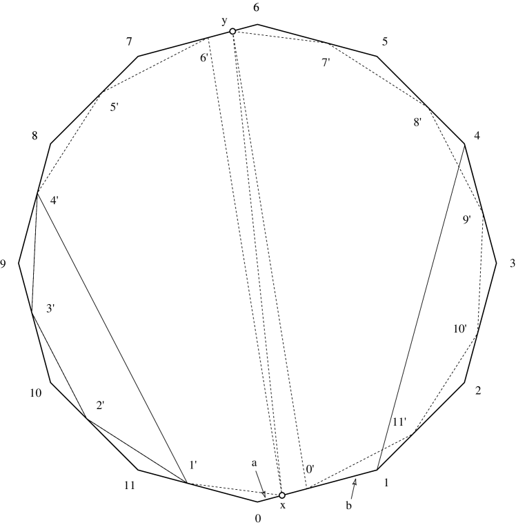
Figure 30: Duodecagon, $n=12$, ${\alpha}=30^{\circ}$, $a\approx 0.2$, $b\approx 0.6$. $x$ and $y$ are perimeter-halving fold vertices. The dashed lines are (largely) conjectured creases. The vertices $v_{i}$, and the gluing points $v^{\prime}_{i}$, are labeled with $i$ and $i^{\prime}$ respectively. The left and right quadrilaterals play a role in Fig. 33 below.

As mentioned in Section 1, we have no method for computing the 3D structure of the unique polytope determined by a particular Aleksandrov gluing. Moreover, we do not even have a general method for computing the creases, i.e., the edges of the polytope. We will therefore largely conjecture the structure of the pita polytopes in this section, although we will establish a subset of the creases. We will only explore the situation for even $n$. Let ${\alpha}=2\pi/n$, the turn angle at each vertex of the polygon.

We view each pita polytope as composed of four parts:

1. A central parallelogram with short side $a$: $(x,v^{\prime}_{0},y,v^{\prime}_{n/2})$.

2. A top, nearly half-$n$-gon: $(v^{\prime}_{0},v^{\prime}_{n-1},v^{\prime}_{n-2},\ldots,v^{\prime}_{n/2+1})$.

3. A bottom, nearly half-$n$-gon, congruent by reflection to the top: $(x,v^{\prime}_{1},v^{\prime}_{2},\ldots,v^{\prime}_{n/2})$.

4. A “mouth,” a strip of triangular teeth; see Fig. 31. $n-2$ of the triangles in the strip are congruent; call their generic shape $T_{1}$. $T_{1}$ has sides of length $b$, $2a$, and $1$, with an angle ${\alpha}$ between $b$ and $2a$. The two extreme triangles of the mouth are smaller, of shape $T_{2}$: lengths $b$ and $a$ surrounding an angle ${\alpha}$.

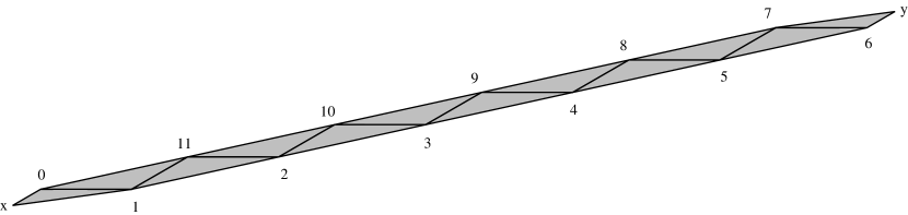
Figure 31: Mouth strip of teeth corresponding to Fig. 30. (Not to same scale.)

We conjecture that the central parallelogram’s edges are creases, as is its central perimeter-splitting diagonal $xy$. Call the top and bottom nearly half-$n$-gons pita polygons. We have no conjectures about how the pita polygons are triangulated (except that they are triangulated the same). Finally, we prove below in Lemma 9.7 that the mouth is creased at the edges displayed in Fig. 31.

The final 3D shape looks something like Fig. 32. As $n\rightarrow\infty$, the polytope approaches a doubly-covered flat semicircle.

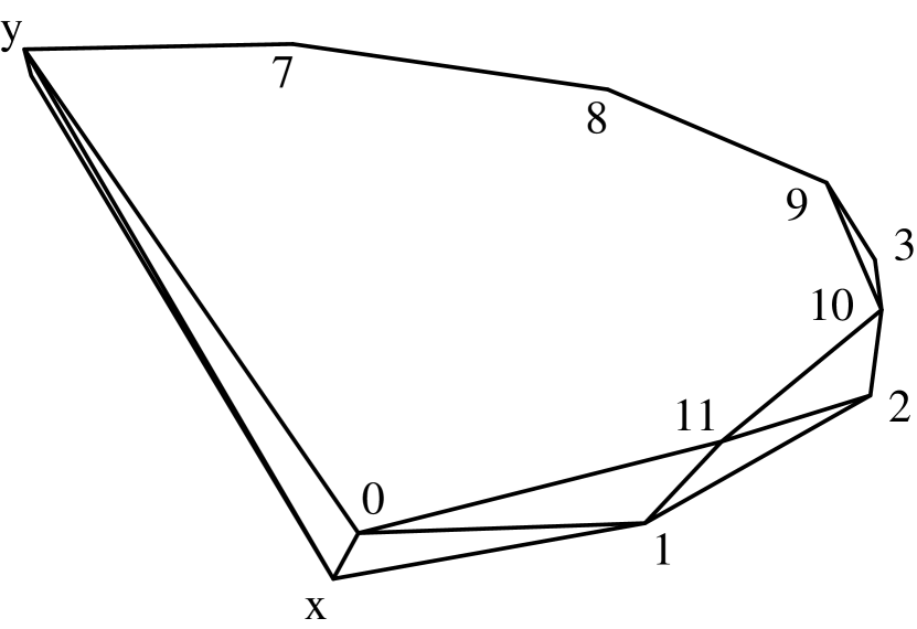
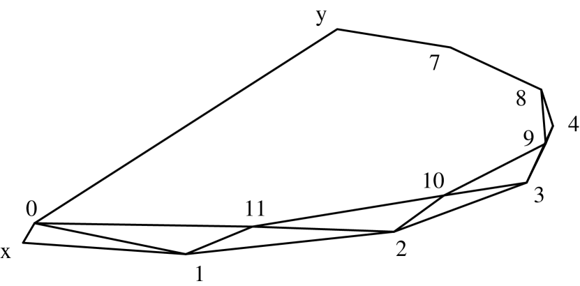
Figure 32: Two views of the approximate 3D shape of pita polytope folded as per Fig. 30.

We now establish the structure of the mouth of pita polytopes. We start with this obvious claim:

Lemma 9.4

Pita polytopes are not flat.

Proof: A flat polytope is a pasting of two congruent polygons, oriented and aligned the same. The vertices of the polygons are the only spots on the polytope surface with curvature. We know the location of all these $n+2$ vertices: $x$, $y$, and $v_{0},\ldots,v_{n-1}$. Thus the two polygons must be $(y,x,v_{1},\ldots,v_{n/2})$ $(x,y,v_{n/2+1},\ldots,v_{0})$. However, because $x$ and $y$ are not at the midpoints of their edges (by definition of a pita polytope), these two polygons are not congruent. $\Box$

Our tools will be two facts about edges of triangulated polytopes, neither of which we will prove:

Fact 9.1

Every edge of a polytope is a shortest path between its endpoint vertices.

Call two polytope edges incident to the same polytope vertex $v$ adjacent if they are consecutive in a circular sorting around $v$.

Fact 9.2

The smaller surface angle between two adjacent edges incident to a polytope vertex is less than $\pi$. In other words, within every open semicircle of face angle at a polytope vertex $v$, there is at least one edge incident to $v$.

We use Fact 9.1 to eliminate certain geodesics as candidates for polytope edges. The following lemma gathers together some basic distance relationships to be used later to show that some geodesics are not shortest paths:

Lemma 9.5

The following distance relationships hold for the length of chords between points of a pita polygon:

1. $|v_{i}-v^{\prime}_{j}|=|v^{\prime}_{i}-v_{j}|$.

2. $|v^{\prime}_{i}-v^{\prime}_{j}|<|v_{i}-v_{j}|$ for all $|i-j|>1$, i.e., for all $j\neq i$ and $j\neq i\pm 1$.

3. $|v^{\prime}_{i}-x|<|v_{i}-x|$ for all $i\neq 0$.

4. $|v^{\prime}_{i}-y|<|v_{i}-y|$ for all $i\neq n/2$.

Proof:

1. The polygons cut off by the chords $(v_{i},v^{\prime}_{j})$ and $(v^{\prime}_{i},v_{j})$ are congruent. For example, in Fig. 30, the chord $(v_{4},v^{\prime}_{0})$ cuts off a polygon of edge lengths $(b,1,1,1)$, and the chord $(v^{\prime}_{4},v_{0})$ cuts off a polygon of lengths $(b,1,1,1)$, both of whose outer interior angles are all ${\alpha}$.

2. Distances between the $v^{\prime}_{i}$ vertices are in general less than distances between the corresponding unprimed vertices, because the primed vertices form a regular figure inscribed in the $n$-gon. A particular instance is illustrated in Fig. 33. For $j=i+1$, the distances are equal.

   

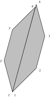
   Figure 33: $|v^{\prime}_{1}-v^{\prime}_{4}|<|v_{1}-v_{4}|$ (cf. Fig. 30).

3. Here the reason is similar: the primed vertices are inscribed in the $n$-gon determined by the unprimed vertices. For example, $|v_{1}-x|=a+b$, but $|v^{\prime}_{1}-x|$ is the length of the hypotenuse of a $T_{2}$ triangle, with sides $a$ and $b$, which is shorter by the triangle inequality. We will not detail the computations necessary to establish this claim for all $i$. The only exception to the inequality is for $v_{0}$, when $|v_{0}-x|=|v^{\prime}_{0}-x|=a$.

4. Symmetric with previous case.

$\Box$

To eliminate the equal-length geodesics in Lemma 9.5(1), we will need the following:

Lemma 9.6

An edge $e=vu$ of a nonflat polytope $Q$ is a uniquely shortest path, i.e., there is not another geodesic of the same length from $v$ to $u$.

Proof: Suppose $e=vu$ is an edge of $Q$. Let $g$ be another geodesic between $v$ and $u$ of the same length as $e$. Then because $e$ is a straight segment in 3D, and because any nonstraight path is strictly longer, it must be that $g$ is also a straight segment in 3D. Thus it must be coincident with $e$. If $e$ and $g$ are nevertheless distinct, then they must be on opposite sides of a flat surface. But then $Q$ must be flat (“pinched”) at $e=g$, which by convexity implies that $Q$ is entirely flat. This contradicts the assumption of the lemma. $\Box$

We now have assembled enough information to pin down the structure of the mouth:

Lemma 9.7

The mouth of a pita polytope is triangulated as in Fig. 31: the edges

$$(x,v_{1},\ldots,v_{n/2},y,v_{n/2+1},\ldots,v_{n-1},v_{0})$$

surrounding the mouth, and the diagonals $(v_{i},v_{n-i})$ and $(v_{n-i+1},v_{i})$ that delimit its “teeth” (cf. Fig. 31), are all polytope edges.

Proof: Let $v_{i}$, $i\in\{1,\ldots,n/2-1\}$ be a vertex of the mouth. (It may help to think of $v_{4}$ in Fig. 30 as a typical $v_{i}$ in this proof.) By Fact 9.2, there must be a polytope edge $e$ incident to $v_{i}$ on the top face in the half plane bounded by the line through $v_{i-1}v_{i}$. By Lemma 9.5(2), the other endpoint of $e$ cannot be any $v_{j}$, $|i-j|>1$, for all those are longer than $|v^{\prime}_{i}-v^{\prime}_{j}|$, the length of an alternate geodesic. So they are not shortest paths, and are ruled out by Fact 9.1. By Lemma 9.5(3-4), the other endpoint of $e$ cannot be $x$ or $y$, for we have restricted $i$ so that $i\neq 0$ and $i\neq n/2$. This leaves $v^{\prime}_{j}$ as a possible endpoint of $e$. But by Lemma 9.5(1), $v_{i}v^{\prime}_{j}$ is not uniquely shortest, which by Lemma 9.6 then implies that $Q$ must be flat, which we know is false by Lemma 9.4.

We have excluded all candidates for the endpoint of $e$ except for $j=i\pm 1$. Because we are examining the semicircle bounded by $v_{i-1},v_{i}$, this leaves $v_{i+1}$ as the only possible endpoint. Thus $v_{i}v_{i+1}$ is an edge of the polytope.

Repeating this argument for the bottom face, $i\in\{n/2+1,\ldots,n-1\}$, establishes the outer boundary of the mouth, excluding the edges incident to $x$ and $y$. Those can be argued similarly. The teeth diagonals are now easy to see. We illustrate with $v_{4}$ in Fig. 30. We have just proved that no edge is incident to $v_{4}$ across the top face. But that top face must be triangulated somehow. The only way to triangulate it without using a diagonal incident to $v_{4}$ is to include the diagonal $v^{\prime}_{9}v^{\prime}_{8}$. This means that $v_{4}v_{8}$ and $v_{4}v_{9}$ are edges of the polytope. $\Box$

References

- [AAOS97] P. K. Agarwal, B. Aronov, J. O’Rourke, and C. A. Schevon. Star unfolding of a polytope with applications. SIAM J. Comput., 26(6):1689–1713, December 1997.
- [Ale58] A. D. Alexandrov. Konvexe Polyeder. Akademie-Verlag, Berlin, West Germany, 1958.
- [AO92] B. Aronov and J. O’Rourke. Nonoverlap of the star unfolding. Discrete Comput. Geom., 8:219–250, 1992.
- [AZ67] A. D. Aleksandrov and U. A. Zalgaller. Intrinsic Geometry of Surfaces. American Mathematical Society, Providence, RI, 1967.
- [BDD+98] T. Biedl, E. Demaine, M. Demaine, A. Lubiw, J. O’Rourke, M. Overmars, S. Robbins, and S. Whitesides. Unfolding some classes of orthogonal polyhedra. In Proc. 10th Canad. Conf. Comput. Geom., pages 70–71, 1998. Fuller version in Elec. Proc. http://cgm.cs.mcgill.ca/cccg98/proceedings/welcome.hml.
- [BDEK99] M. Bern, E. D. Demaine, D. Eppstein, and E. Kuo. Ununfoldable polyhedra. In Proc. 11th Canad. Conf. Comput. Geom., pages 13–16, 1999. Full version: LANL archive paper number cs.CG/9908003.
- [Hen79] M. Henle. A Combinatorial Introduction to Topology. W. H. Freeman, San Francisco, CA, 1979.
- [LO96] A. Lubiw and J. O’Rourke. When can a polygon fold to a polytope? Technical Report 048, Dept. Comput. Sci., Smith College, June 1996. Presented at AMS Conf., 5 Oct. 1996.
- [McK83] B. D. McKay. Spanning trees in regular graphs. Europ. J. Combin., 4:149–160, 1983.
- [O’R00] J. O’Rourke. Folding and unfolding in computational geometry. In Proc. Japan Conf. Discrete Comput. Geom. ’98, volume 1763 of Lecture Notes Comput. Sci., page 258–266 Springer-Verlag, 2000.
- [She75] G. C. Shephard. Convex polytopes with convex nets. Math. Proc. Camb. Phil. Soc., 78:389–403, 1975.