Interval Constraint Solving
for Camera Control and Motion Planning

Abstract

Many problems in robust control and motion planning can be reduced to either find a sound approximation of the solution space determined by a set of nonlinear inequalities, or to the “guaranteed tuning problem” as defined by Jaulin and Walter, which amounts to finding a value for some tuning parameter such that a set of inequalities be verified for all the possible values of some perturbation vector. A classical approach to solve these problems, which satisfies the strong soundness requirement, involves some quantifier elimination procedure such as Collins’ Cylindrical Algebraic Decomposition symbolic method. Sound numerical methods using interval arithmetic and local consistency enforcement to prune the search space are presented in this paper as much faster alternatives for both soundly solving systems of nonlinear inequalities, and addressing the guaranteed tuning problem whenever the perturbation vector has dimension one. The use of these methods in camera control is investigated, and experiments with the prototype of a declarative modeller to express camera motion using a cinematic language are reported and commented.

The research exposed here was supported in part by the INRIA LOCO project and a project of the French/Russian A.M. Liapunov Institute.

This is a revised and extended version of a paper presented at the sixth International Conference on Principles and Practice of Constraint Programming (CP ’00), Singapore.

1 Introduction

Designing electronic circuits [Ebers and Moll (1954)], identifying the structure of complex molecules [Emiris and Mourrain (1999)], or computing the quantity of chemical elements produced by some reaction [Meintjes and Morgan (1990)] are all problems—among many others—that can be modelled by sets of real nonlinear equations and inequations. Reliably solving these systems (that is, delivering approximate solutions as close as possible to the true ones) with the limited set of real numbers representable on computers has generated a large amount of literature since the very dawn of computer science [Turing (1948), Rademacher (1948), Wilkinson (1963)].

Following Sunaga’s and Moore’s seminal works [Sunaga (1958), Moore (1966)], interval analysis has been identified as a key tool for ensuring reliability and completeness (that is, the capability to retain all the solutions) in the solving process.

Interval constraint solving [Older and Vellino (1990), Benhamou (1995)] uses interval arithmetic in algorithms alternating propagation steps [Waltz (1975), Mackworth (1977)], which enforce some local consistency notion to tighten the variables’ feasible domain, and search steps to isolate different solutions and overcome the weakness of the propagation steps.

Interval constraint solvers such as clp(BNR) [Benhamou and Older (1997)], ILOG Solver [Puget (1994)], or Numerica [Van Hentenryck et al. (1997)] have been shown to be efficient tools for solving some challenging nonlinear constraint systems [Puget and Van Hentenryck (1998), Granvilliers and Benhamou (2001)]). Relying on interval arithmetic, they guarantee completeness and isolate punctual solutions with an “arbitrary” accuracy. They take as input a constraint system and a Cartesian product of domains for the variables occurring in the constraints; their output is a set $\mathcal{S}_{o}$ of boxes approximating each solution contained in the input box.

However, soundness (i.e., the property that all boxes returned contain nothing but true solution points) is not guaranteed while it is sometimes a strong requirement. Consider, for instance, a civil engineering problem [Sam (1995)] such as floor design where retaining non-solution points may lead to a physically infeasible structure. As pointed out by Ward et al. [Ward et al. (1989)] and Shary [Shary (1999)], one may expect different properties from the boxes composing $\mathcal{S}_{o}$ depending on the problem at hand, namely: every element in any box is a solution, or there exists at least one solution in each box. Interval constraint solvers ensure only, at best, the second property.

Interval constraint solving techniques also suffer from a severe limitation in that they can only handle constraint systems with discrete solutions. Yet, many applications in robust control or error-bounded estimation [Jaulin and Walter (1993)] are modelled by systems of nonlinear inequalities, whose solution set is usually not discrete.

In addition, even more applications can be reduced to what Jaulin and Walter [Jaulin and Walter (1996)] call the “guaranteed tuning problem”, which amounts to finding the values for some tuning parameter such that a set of inequalities be verified for all the possible values of some perturbation vector. More precisely:

Given $\mathbf{B}$, a box of feasible values for some tuning parameter vector $\boldsymbol{\gamma}$ and $\mathbf{D}$, a box of feasible values for some perturbation vector $\boldsymbol{\pi}$, find the set $\mathcal{S}_{\boldsymbol{\gamma}}$ defined by:

$$\mathcal{S}_{\boldsymbol{\gamma}}=\{\boldsymbol{\gamma}\in\mathbf{B}\mid\forall\boldsymbol{\pi}\in\mathbf{D}\colon\mathbf{f}(\boldsymbol{\gamma},\boldsymbol{\pi})\geqslant\mathbf{0}\}$$

where $\mathbf{f}$ is a vector of nonlinear functions, and the inequality is to be taken componentwise.

Problems ranging from robust control [Abdallah et al. (1996)] and camera control [Drucker and Zeltzer (1994)] to motion planning [Tarabanis (1990)] can all be formulated as guaranteed tuning problems. Consider for example the following application:

Example 1.1 (A collision-free problem).

A mobile robot arm is composed of three segments of respective lengths $d_{1}$, $d_{2}$ and $d_{3}$, and three motor-controlled axes (see Figure 1). The trajectory of the robot’s hand $P(t)$ is therefore determined by three angle functions $\alpha_{1}(t)$, $\alpha_{2}(t)$ and $\alpha_{3}(t)$. The problem is to find all points in the $2D$ space that do not collide with the robot’s hand, i.e. computing all the $(x,y)$ coordinates such that the distance between $P(t)$, for all $t$, and $(x,y)$ is greater than some given value $d$ (here, the size of the robot’s hand):

$$\forall t\in[0,1]\colon\sqrt{(x-P_{x}(t))^{2}+(y-P_{y}(t))^{2}}\geqslant d$$

where $P_{x}(t)$ and $P_{y}(t)$ represent the coordinates of $P(t)$ at time $t$, defined by:

$$\left\{\begin{array}[]{ll}P_{x}(t)=&d_{1}\sin\alpha_{1}(t)+d_{2}\sin\bigl{(}\alpha_{1}(t)+\alpha_{2}(t)-\pi\bigr{)}+d_{3}\sin\bigl{(}\alpha_{1}(t)+\alpha_{2}(t)+\alpha_{3}(t)\bigr{)}\\ P_{y}(t)=&d_{1}\cos\alpha_{1}(t)+d_{2}\cos\bigl{(}\alpha_{1}(t)+\alpha_{2}(t)-\pi\bigr{)}+d_{3}\cos\bigl{(}\alpha_{1}(t)+\alpha_{2}(t)+\alpha_{3}(t)\bigr{)}\\ \end{array}\right.$$

Figure 1: Avoiding collisions with the arm of a robot

Until recently, the soundness issue and the presence of quantifiers called for symbolic methods and quantifier elimination procedures such as Cylindrical Algebraic Decomposition [Collins (1975)] (CAD). Unfortunately, these techniques are either too slow, or limited to polynomial constraints.

The advent of interval analysis led to the devising of simple and sound algorithms to solve systems of inequalities [Jaulin and Walter (1993), Garloff and Graf (1999)] and the guaranteed tuning problem (restricted to the finding of only one value, though) [Jaulin and Walter (1996)]. By and large, many of these algorithms are but sophisticated interval extensions of simple search procedures, meaning that are they computationally expensive, even for small problems.

In this paper, we present sound algorithms that draw upon efficient complete interval constraint solving pruning methods to soundly solve systems of inequalities and the guaranteed tuning problem for the case of unidimensional perturbation vectors. This kind of problem is the one occurring in motion planning and camera control applications, where the only universally quantified variable is usually the time.

The outline of the paper is as follows: in order to be reasonably self-content, the basics of interval analysis are presented in Section 2; related works on both solving systems of nonlinear inequalities and the guaranteed tuning problem are presented in Section 3; their strong points and weaknesses regarding the applications targeted are also pointed out; interval constraint solving is introduced in Section 4 as a basis for the new sound algorithms presented in Section 5; the modelling of a camera control problem in terms of these new sound interval constraint methods is then described in Section 6; the results with a prototype of a declarative modeller allowing a non-technician user to control the positioning of a camera by means of a cinematic language are commented in Section 7 and contrasted with the ones obtained by Jardillier and Languénou [Jardillier and Languénou (1998)] on the same problems with a different approach; finally, Section 8 discusses directions for future researches.

2 Interval Analysis

In this section, we limit the presentation of interval analysis to the concepts needed in the sequel of the paper. The reader is referred to works by Moore, Hansen and others [Moore (1966), Alefeld and Herzberger (1983), Hansen (1992), Neumaier (1990)] for a more complete presentation.

The finite nature of computers implies that they can only represent and manipulate a small subset of the real numbers represented in a floating-point format. Since the mid-eighties, most computers comply with the IEEE 754 standard [IEEE (1985)] specifying the format of floating-point numbers.

The set of floating-point numbers $\mathbb{F}$ is but a very small subset of real numbers. In addition, it is not closed for arithmetic operations, meaning that rounding of the results to representable floating-point numbers must usually take place. We say that an operation is correctly rounded when the value chosen, whenever the true result is not representable, is the closest floating-point number. Note that the IEEE 754 standard only requires the operators $+,-,\times,\div,\sqrt{\>}$ to be correctly rounded. The precision of the other operators is implementation dependent. See the paper by Lefèvre et al. [Lefèvre et al. (1998)] for more information on this topic.

Given a floating-point number $a$, let ${a}^{+}$ (resp. ${a}^{-}$) be the smallest float greater than $a$ (resp. greatest float smaller than $a$).

Rounding makes the reliable solving of systems of nonlinear equalities or inequalities a challenging task, to which a large amount of papers and books has been devoted.

One solution advocated by Moore [Moore (1966)] to control the rounding errors is to use interval arithmetic, that is to replace reals by intervals containing them, whose bounds are representable numbers. For example:

$$\pi\in[3.14,3.15]$$

An interval $I$ with representable bounds is called a floating-point interval. It is of the form: $I=[a,b]=\{r\in\mathbb{R}\mid a\leqslant r\leqslant b,\>\text{with}\>\>a,b\in\mathbb{F}\}$. A non-empty interval $I=[a,b]$ such that $b\leqslant{a}^{+}$ is said canonical. In the same way, a Cartesian product of intervals (or box) is said canonical whenever it is canonical in all its dimensions. In the sequel, vectors or Cartesian products are written in bold face.

Let $\mathbb{I}$ be the set of all floating-point intervals. Since we will only deal with this kind of intervals in the rest of the paper, we will refer to them as simply intervals.

Operations and functions over reals are also replaced by an interval extension having the containment property. Given a real function, $f\colon\mathbb{R}^{n}\to\mathbb{R}$ and a box $\mathbf{B}\in\mathbb{I}^{n}$, let $f(\mathbf{B})=\{f(\mathbf{r})\mid\mathbf{r}\in\mathbf{B}\}$, $\mathcal{D}_{f}$ be the domain of $f$, and $\mathcal{D}^{\mathbb{I}}_{f}=\{\mathbf{B}\in\mathbb{I}^{n}\mid\mathbf{B}\subseteq\mathcal{D}_{f}\}$.

Definition 2.1 (Interval extension).

Given a real function $f\colon\mathbb{R}^{n}\to\mathbb{R}$, an interval extension $F\colon\mathbb{I}^{n}\to\mathbb{I}$ of $f$ is an interval function verifying:

$${\textsf{Outer}}(f(\mathbf{B})) \subseteq F(\mathbf{B}) \forall\mathbf{B}\in\mathcal{D}^{\mathbb{I}}_{f}$$

where ${\textsf{Outer}}(\rho)=\bigcap\{\mathbf{B}\in\mathbb{I}^{n}\mid\rho\subseteq\mathbf{B}\}$ for any real relation $\rho\subseteq\mathbb{R}^{n}$.

The extensions of some basic operators are defined as follows:

$$\begin{array}[]{ll}[a,b]+[c,d]=&[a+c,b+d]\\ [a,b]-[c,d]=&[a-d,b-c]\\ [a,b]\times[c,d]=&[\min(ac,ad,bc,bd),\max(ac,ad,bc,bd)]\\ \exp([a,b])=&[\exp(a),\exp(b)]\end{array}$$

Note that in practice, the bounds computed have to be outward rounded in order to preserve the containment property.

A particular interval extension, the natural interval extension is obtained by replacing syntactically in a real function all the real constants by intervals containing them, all the real variables by interval variables, and all operators by their interval extension.

Interval arithmetic is commutative, but it is neither associative (due to floating-point numbers wanting for this property themselves), nor distributive. It enjoys instead a sub-distributive property, namely:

$$\forall I,J,K\in\mathbb{I}\colon\quad I(J+K)\subseteq IJ+IK$$

The sub-distributivity property has an important impact in that equivalent forms for a function over reals may not have equivalent natural extensions.

In the rest of this paper, we will often consider the set of real numbers represented by a set of Cartesian product of intervals. Given $\mathcal{P}(\mathcal{S})$ the power set of any set $\mathcal{S}$, we then introduce the operator $\Lbag{\cdot}\Rbag\colon\mathcal{P}(\mathbb{I}^{n})\to\mathbb{R}^{n}$ defined as follows:

$$\forall\mathbf{B_{1}},\dots,\forall\mathbf{B_{n}}\in\mathbb{I}^{n}\colon\Lbag{\{\mathbf{B_{1}},\dots,\mathbf{B_{n}}\}}\Rbag=\{\mathbf{r}\in\mathbb{R}^{n}\mid\exists i\in\{1,\dots,n\}\text{ s.t. }\mathbf{r}\in\mathbf{B_{i}}\}$$

Lastly, given a box $\mathbf{B}=I_{1}\times\cdots\times I_{n}$, an integer $k\in\{1,\dots,n\}$, and an interval $J$, let $\mathbf{B}_{{I_{k}}\mathbin{\leftarrow}{J}}=I_{1}\times\cdots\times I_{k-1}\times J\times I_{k+1}\times\cdots\times I_{n}$ be the box $\mathbf{B}$ where $I_{k}$ has been replaced by $J$.

3 Related Work

Computing a subpaving (Figure 2) of a real relation $\rho\subseteq\mathbb{R}^{n}$ consists in partitionning $\mathbb{R}^{n}$ into three sets $(\mathcal{U}_{i},\mathcal{U}_{o},\mathcal{U}_{u})$ of non-overlapping boxes with the properties:

$$\left\{\begin{array}[]{l}\Lbag{\mathcal{U}_{i}}\Rbag\subseteq\rho\\ \Lbag{\mathcal{U}_{o}}\Rbag\cap\rho=\varnothing\\ \Lbag{\mathcal{U}_{i}\cup\mathcal{U}_{u}}\Rbag\supseteq\rho\end{array}\right.$$ (1)

Given an $n$-ary constraint $c$, let $\rho_{c}\subseteq\mathbb{R}^{n}$ be the underlying relation, that is:

$$\rho_{c}=\{(r_{1},\dots,r_{n})\in\mathbb{R}^{n}\mid c(r_{1},\dots,r_{n})\}$$

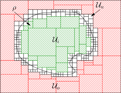
Figure 2: Subpaving of the relation $\rho$

Given an $n$-ary constraint $c$ and a box $\mathbf{B}\in\mathbb{I}^{n}$, and assuming the existence of some procedure GlobSat with the following properties:

$$\left\{\begin{array}[]{ll}{\textsf{GlobSat}}(c,\mathbf{B})=\text{true}&\implies\mathbf{B}\subseteq\rho_{c}\\ {\textsf{GlobSat}}(c,\mathbf{B})=\text{false}&\implies\mathbf{B}\cap\rho_{c}=\varnothing\\ {\textsf{GlobSat}}(c,\mathbf{B})=\text{unknown}&\implies???\end{array}\right.$$

it is easy to devise a systematic procedure to compute the subpaving of $\rho_{c}$ by alternating evaluation steps with GlobSat, and splitting steps whenever GlobSat returns “unknown.” The precise algorithm is presented in Table 2 for a conjunction of constraints.

1	Subpaving$\bigl{(}$: $\{c_{1},\dots,c_{m}\}$, $\mathbf{B}\in\mathbb{I}^{n}$; : $(\mathcal{U}_{i},\mathcal{U}_{o},\mathcal{U}_{u})\in\mathcal{P}(\mathbb{I}^{n})^{3}\bigr{)}$
2
3		sat $\leftarrow{\textsf{GlobSat}}(c_{1},\mathbf{B})\wedge\cdots\wedge{\textsf{GlobSat}}(c_{m},\mathbf{B})$
4		sat
5			:
6				$(\{\mathbf{B}\},\varnothing,\varnothing)$
7			:
8				$(\varnothing,\{\mathbf{B}\},\varnothing)$
9			:
10				StoppingCriterion$(\mathbf{B})~{}$
11					$(\varnothing,\varnothing,\{\mathbf{B}\})$
12
13					$(\mathbf{B_{1}},\dots,\mathbf{B_{k}})\leftarrow{\textsf{Split}}_{k}(\mathbf{B})$
14					$\displaystyle\biguplus_{j=1}^{k}{\textsf{Subpaving}}(\{c_{1},\dots,c_{m}\},\mathbf{B_{j}})$
15
16
17

Subpaving algorithm for a conjunction of atomic constraints $c_{1}\wedge\cdots\wedge c_{m}$

The StoppingCriterion function appearing on Line $10$ of Alg. Subpaving returns “true” or “false” depending whether the box given as an argument should still be considered for splitting. A typical instance of this method is testing for canonicity of the box. It is also possible to speed-up the computation by using another instance of StoppingCriterion that would avoid splitting boxes whose width is smaller than some $\varepsilon$.

The ${\textsf{Split}}_{k}$ function on Line $13$ splits a box $\mathbf{B}$ into $k$ non-overlapping subboxes whose union is equal to $\mathbf{B}$.

The $\biguplus$ operator on Line $14$ applies on vectors of sets and performs their unions componentwise:

$$\biguplus_{i}\biggl{\{}(\mathcal{S}_{1}^{i},\dots,\mathcal{S}_{n}^{i})\biggr{\}}=(\bigcup_{i}\mathcal{S}_{1}^{i},\dots,\bigcup_{i}\mathcal{S}_{n}^{i})$$

The subpaving algorithm has been used by several authors to compute sound boxes for systems of inequalities. They differ by the way they implement the GlobSat method.

In SIVIA, Jaulin and Walter [Jaulin and Walter (1993)] use interval arithmetic containment properties: given a constraint $c\colon f(x_{1},\dots,x_{n})\leqslant 0$, and a box $\mathbf{B}$, they evaluate the natural interval extension of $f$ over $\mathbf{B}$. If the right bound of the result is negative, GlobSat returns “true”; if the left bound is strictly positive GlobSat returns “false”; otherwise it returns “unknown.” SIVIA is able to process any kind of inequality constraints, be they linear or not, polynomial or not. The drawback of this approach is that for unstable $f$ functions, the natural interval evaluation leads to large intervals that do not permit deciding whether the box $\mathbf{B}$ is included in $\rho_{c}$ or not. It is then necessary to split the box a lot.

Jaulin and Walter [Jaulin and Walter (1996)] have also devised an algorithm to solve the guaranteed tuning problem (restricted to the finding of only one value). It is based on SIVIA, and then, it suffers from the same drawbacks as SIVIA itself.

The algorithm described by Kutsia and Schicho [Kutsia and Schicho (1999)] implements another instance of Subpaving where GlobSat is obtained by testing some criterion using floating-point numbers of arbitrary precision. An important limitation is that their algorithm can only handle polynomial strict inequalities.

Garloff and Graf [Garloff and Graf (1999)] also restrict themselves to polynomial strict inequalities. They expand the polynomial inequalities into Bernstein polynomials: let $\mathbf{I}=(i_{1},\dots,i_{n})$ be a multi-index (vector of non-negative integers), and $\mathbf{x^{\mathbf{I}}}=x_{1}^{i_{1}}\dots x_{n}^{i_{n}}$ be a monomial. Given a polynomial $p\in\mathbb{R}[x_{1},\dots,x_{n}]$, let $\mathcal{S}$ be a set of multi-indices such that: $p(\mathbf{x})=\sum_{\mathbf{I}\in\mathcal{S}}a_{\mathbf{I}}\mathbf{x}^{\mathbf{I}}$. For any $n$-ary Cartesian product of domains $\mathbf{D}$, one can express $p$ in terms of Bernstein coefficients:

$$p(\mathbf{x})=\sum_{{\mathbf{I}}\in\mathcal{S}}b_{\mathbf{I}}(\mathbf{D})B_{N,{\mathbf{I}}}(\mathbf{x})$$

where $B_{N,{\mathbf{I}}}(\mathbf{x})$ is the ${\mathbf{I}}$th Bernstein polynomial of degree $N$.

It is then well known that the following property does hold [Farouki and Rajan (1987)]:

$$\forall\mathbf{a}\in\mathbf{D}\colon\min_{{\mathbf{I}}\in\mathcal{S}}b_{\mathbf{I}}(\mathbf{D})\leqslant p(\mathbf{a})\leqslant\max_{{\mathbf{I}}\in\mathcal{S}}b_{\mathbf{I}}(\mathbf{D})\quad\text{\emph{(convex hull property)}}$$

As a consequence, it is possible to accurately bound the range of $p(\mathbf{x})$ on every box, and then to know whether an inequality such as $p(\mathbf{x})<0$ does hold or not. By splitting the initial box and evaluating the corresponding Bernstein coefficients, one can isolate all the boxes verifying a set of inequality constraints.

Sam-Haroud and Faltings [Haroud and Faltings (1994)] do not rely on Alg. Subpaving. Instead, they represent explicitly the subpaving of the relation $\rho_{c}$ associated to each $n$-ary inequality constraint by a $2^{n}$-tree of boxes. The category of each box (in $\mathcal{U}_{i}$, $\mathcal{U}_{o}$, or $\mathcal{U}_{u}$) is determined by finding the intersection of the curve with the edges of the box. Sets of constraints are handled by performing intersections of the respective $2^{n}$-trees. In order to avoid a combinatorial explosion, $n$ must be small. As a consequence, they have chosen to decompose the user’s constraints into ternary constraints, so that they only manipulate octrees. The original algorithm is able to compute inner approximations (that is, subsets) of the solution space; on the other hand, it is not designed to handle the guaranteed tuning problem.

The method presented by Collavizza et al. [Collavizza et al. (1999)] is strongly related to the one we present in the following, since they rely on usual interval constraint solving techniques to compute sound boxes for some constraint system. Starting from a seed that is known to belong to the solution space, they enlarge the domain of the variables around it in such a way that the new box computed is still included in the solution space. They do so by using local consistency techniques to find the points at which the truth value of the constraints change. Their algorithm is particularly well suited for the applications they target, viz. the enlargement of tolerances. It is however not designed to solve the guaranteed tuning problem. In addition, it is necessary to obtain a seed for each connected subset of the solution space, and to apply the algorithm on each seed if one is interested in computing several solutions (e.g. to ensure representativeness of the samples).

In order to tighten a box $\mathbf{B}$ of variables’ domains for a problem of the form $\forall v\in I_{k}\colon c_{1}\wedge\cdots\wedge c_{m}$, Jardillier and Languénou [Jardillier and Languénou (1998)] compute an inner approximation by decomposing the initial domain $I_{k}$ of $v$ into canonical intervals $I_{k}^{1}$,…,$I_{k}^{p}$, and testing whether $c_{1}\wedge\cdots\wedge c_{m}$ does hold for the boxes $I_{1}\times\cdots\times I_{k}^{1}\times\cdots\times I_{n}$,…, $I_{1}\times\cdots\times I_{k}^{p}\times\cdots\times I_{n}$. These evaluations give results in a three-valued logic (true, false, unknown). Boxes labeled true contain only solutions, boxes labeled false contain no solution at all, and boxes labeled unknown are recursively split and re-tested until they may be asserted true or false, or canonicity is reached (see Figure 3). Retained boxes are those verifying:

$$\forall j\in\{1,\dots,p\}\colon\left\{\begin{array}[]{l}{\textsf{GlobSat}}(c_{1},I_{1}\times\cdots\times I_{k}^{j}\times\cdots\times I_{n})=\text{true}\\ \wedge\\ \dots\\ \wedge\\ {\textsf{GlobSat}}(c_{m},I_{1}\times\cdots\times I_{k}^{j}\times\cdots\times I_{n})=\text{true}\end{array}\right.$$

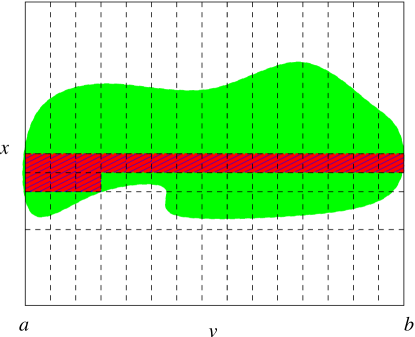
Figure 3: JLA algorithm: solving $\forall v\in[a,b]\colon c(x,v)$

1	JLA$\bigl{(}$: $\{c_{1},\dots,c_{m}\}$, $\mathbf{B}\in\mathbb{I}^{n}$, a variable $v$, $l\in\mathbb{F}$; : $(\mathcal{U}_{i},\mathcal{U}_{o},\mathcal{U}_{u})\in\mathcal{P}(\mathbb{I}^{n})^{3}\bigr{)}$
2
3		$\mathbf{B^{\prime}}\leftarrow\mathbf{B}_{{I_{v}}\mathbin{\leftarrow}{[l,{l}^{+}]}}$
4		sat $\leftarrow{\textsf{GlobSat}}(c_{1},\mathbf{B})\wedge\cdots\wedge{\textsf{GlobSat}}(c_{m},\mathbf{B})$
5		sat
6			:
7				${l}^{+}=\overline{v}$
8					$(\{\mathbf{B}\},\varnothing,\varnothing)$
9
10					JLA$(\{c_{1},\dots,c_{m}\},\mathbf{B},v,{l}^{+})$
11
12			:
13				$(\varnothing,\{\mathbf{B}\},\varnothing)$
14			:
15				${\textsf{StoppingCriterion}}(\mathbf{B})$
16					$(\varnothing,\varnothing,\{\mathbf{B}\})$
17
18					$(\mathbf{B_{1}},\dots,\mathbf{B_{k}})\leftarrow{\textsf{Split}}^{\setminus v}_{k}(\mathbf{B})$
19					$\displaystyle\biguplus_{j=1}^{k}{\textsf{JLA}}(\{c_{1},\dots,c_{m}\},\mathbf{B_{j}},v,l)$
20
21
22

Evaluation-based propagation algorithm for $\forall v\in[\underline{v},\overline{v}]\colon c_{1}\wedge\cdots\wedge c_{m}$

The precise algorithm is described in Table 3. In the initial call, the $l$ parameter is equal to the left bound of $v$’s domain. The ${\textsf{Split}}^{\setminus v}_{k}$ procedure in Line $18$ is identical to the ${\textsf{Split}}_{k}$ procedure presented previously, except that it never splits the domain of the universally quantified variable $v$.

Once again, Alg. JLA is but a sophisticated instance of Alg. Subpaving, which means that its efficiency strongly depends on the quality of the GlobSat procedure. Like in SIVIA, Jardillier and Languénou use the natural interval extension of the constraints. As a consequence, their algorithm is computationally expensive in many cases, as soon as some moderate precision in the computation of the inner approximation is required. We refer the reader to Section 7 for precise figures.

Due to lack of space, we will not present the Cylindrical Algebraic Decomposition method for quantifier elimination here, and we refer the reader to the good introduction by Jirstrand [Jirstrand (1995)].

4 Interval Constraint Solving

Since finite representation of numbers by computers hinders the reliable solving of real equations and inequations, interval constraint solving relies on interval arithmetic [Moore (1966), Alefeld and Herzberger (1983)] to compute verified approximate solutions of real constraint systems.

The reader will find in various works [Older and Vellino (1990), Benhamou and Older (1997), Benhamou (1996), Van Hentenryck et al. (1997), Benhamou et al. (1994), Van Hentenryck et al. (1997), Benhamou et al. (1999)] a thorough presentation of the interval constraint solving framework and of the associated state-of-the-art algorithms. In this section, we will describe only the elements that are essential to our purpose. In particular, we will restrict ourselves to the case of nonlinear inequality constraints only, that is constraints of the form $f(x_{1},\dots,x_{n})\leqslant 0$ for some real function $f$.

Proofs not given here may be found in the papers cited above.

4.1 Local Consistencies

Discarding all inconsistent values from a box of variables’ domains is intractable when the constraints are real ones (consider for instance the constraint $c\colon\sin(x)=1,\quad x\in[0,2]$). Consequently, weak consistencies have been devised, among which one may cite hull consistency [Benhamou (1995)] and box consistency [Benhamou et al. (1994)]. Both consistencies permit narrowing variables’ domains to (hopefully) smaller domains, preserving all the solutions present in the input. Since they are used as a basis for the algorithms to be introduced in Section 5, they are both presented below.

Discarding values of the variable domains for which $c$ does not hold according to a given consistency notion is modelled by means of outer contracting operators, whose main properties are contractance, completeness, and monotonicity.

4.1.1 Outer Contracting Operators

Depending on the considered consistency, one may define different contracting operators for a constraint. In this section, hull consistency and box consistency are first formally presented. Operators based on both consistencies are then given.

Hull consistency is a strong “weak consistency” since a constraint $c$ is said hull consistent w.r.t. a box whenever that box cannot be tightened without losing some solutions for $c$:

Definition 4.1 (Hull consistency).

A real constraint $c(x_{1},\dots,x_{n})$ is said hull-consistent w.r.t. a box $\mathbf{B}=I_{1}\times\cdots\times I_{n}$ if and only if:

$$\forall k\in\{1,\dots,n\}\colon\\ I_{k}\mathrel{=}{\textsf{Outer}}(I_{k}\cap\{r_{k}\in\mathbb{R}\mid\forall j\in\{1,\dots,n\}\setminus\{k\}\colon\\ \exists r_{j}\in I_{j}\text{ s.t. }(r_{1},\dots,r_{n})\in\rho_{c}\})$$

An operator enforcing hull consistency for a constraint $c$ computes the smallest box containing the intersection of the input box and the relation $\rho_{c}$:

Definition 4.2 (Outer-hull contracting operator).

Let $c$ be an $n$-ary constraint, $\rho_{c}$ its underlying relation, and $\mathbf{B}$ a box. An outer-hull contracting operator for $c$ is a function ${\textsf{HC}}_{c}\colon\mathbb{I}^{n}\to\mathbb{I}^{n}$ defined by:

$${\textsf{HC}}_{c}(\mathbf{B})={\textsf{Outer}}(\mathbf{B}\cap\rho_{c})$$

Proposition 4.3 (Completeness of HC)

Given a constraint $c$ and a box $\mathbf{B}$, the following relation does hold: $(\mathbf{B}\cap\rho_{c})\subseteq{\textsf{HC}}_{c}(\mathbf{B})$.

Operationally, hull consistency is enforced over constraints by decomposing them into conjunctions of primitive constraints. The drawback of such a method lies in the loss of domain tightening due to the introduction of new variables during the decomposition process. Box consistency has been introduced by Benhamou et al. [Benhamou et al. (1994)] to overcome this problem: the operators enforcing box consistency consider constraints globally, without decomposing them.

Definition 4.4 (Box consistency).

Let $c$ be an $n$-ary real constraint, $C$ an interval extension for $c$, and $\mathbf{B}=I_{1}\times\cdots\times I_{n}$ a box. The constraint $c$ is said box-consistent w.r.t. $\mathbf{B}$ if and only if:

$$\forall k\in\{1,\dots,n\}\colon\\ I_{k}={\textsf{Outer}}(I_{k}\cap\{r\in\mathbb{R}\mid C(I_{1},\dots,I_{k-1},{\textsf{Outer}}(\{r\}),I_{k+1},\dots,I_{n})\})$$

Intuitively, a constraint $c$ is box-consistent w.r.t. a box $\mathbf{B}$ when each projection $I_{j},j\in\{1,\dots,n\}$ of $\mathbf{B}$ is the smallest interval containing all the elements that cannot be distinguished from solutions of the univariate constraint obtained from $C$ by replacing all the variables but $x_{j}$ by their current domain due to the inherently limited precision of the computation with floating-point numbers.

Box consistency is enforced over a constraint $c(x_{1},\dots,x_{n})$ as follows: $n$ contracting operators (typically using an interval Newton method [Van Hentenryck et al. (1997)]) are associated to the $n$ univariate interval constraints obtained as described above. The $k$th operator reduces the domain of $x_{k}$ by computing the leftmost and rightmost canonical intervals $J$ such that $C(I_{1},\dots,I_{k-1},J,I_{k+1},\dots,I_{n})$ does hold (leftmost and rightmost quasi-zeros).

Using box consistency to narrow down the variable domains of a constraint leads to the notion of outer-box contracting operator:

Definition 4.5 (Outer-box contracting operator).

Given an $n$-ary constraint $c$ and a box $\mathbf{B}$, an outer-box contracting operator ${\textsf{BC3r}}_{c}\colon\mathbb{I}^{n}\to\mathbb{I}^{n}$ for $c$ is defined by:

$${\textsf{BC3r}}_{c}(\mathbf{B})=\max\{\mathbf{B^{\prime}}\mid\mathbf{B^{\prime}}\subseteq\mathbf{B}\\ \text{ and }c\text{ is box-consistent w.r.t. }k\in\{1,\dots,n\}\text{ and }\mathbf{B^{\prime}}\}$$

Proposition 4.6 (Completeness of BC3r)

Given a constraint $c$, the following relation does hold for any box $\mathbf{B}$:

$$(\mathbf{B}\cap\rho_{c})\subseteq{\textsf{BC3r}}_{c}(\mathbf{B})$$

Consistencies and associated contracting operators considered so far are such that completeness is guaranteed (no solution lost during the narrowing process). Devising operators that ensure soundness of the results is the topic of the next section.

5 Sound Interval Constraint Solving

We have seen in the previous section some operators that compute an outer approximation of the relation $\rho$ associated to some nonlinear constraint system. In this section, we will present operators that compute an inner approximation of $\rho$, that is, a subset of the solution space of the corresponding constraint system. As a consequence, the boxes computed by these operators will have the property that any point inside of them is a true solution to the problem, thus ensuring soundness of the results given to the user.

Several definitions for the inner approximation of a real relation exist in the literature, depending on the intended application. Given an $n$-ary relation $\rho$, one may single out at least the two following definitions for an inner approximation ${\textsf{Inner}}(\rho)$ of $\rho$:

1. Def. A. ${\textsf{Inner}}(\rho)=\mathbf{B_{1}}$, where $\mathbf{B_{1}}\in\{\mathbf{B}\in\mathbb{I}^{n}\mid\mathbf{B}\subseteq\rho\}$ (an inner-approximation is any box included in the relation) [Markov (1995), Armengol et al. (1998)];

2. Def. B. ${\textsf{Inner}}(\rho)=\mathbf{B_{1}}$, where $\mathbf{B_{1}}\in\{\mathbf{B}=I_{1}\times\cdots\times I_{n}\mid\mathbf{B}\subseteq\rho\wedge\forall j\in\{1,\dots,n\},\forall I^{\prime}_{j}\supseteq I_{j}\colon\mathbf{B}_{{I_{j}}\mathbin{\leftarrow}{I^{\prime}_{j}}}\subseteq\rho\implies I^{\prime}_{j}=I_{j}\}$ (an inner-approximation is a box included in the relation that cannot be extended in any direction without containing non-solution points) [Shary (1999)].

Definitions A and B imply that disconnected relations are only very partially represented by one box only, a drawback that is avoided with the following stronger definition, which will be used in this paper:

Definition 5.1 (Inner approximation operator).

Given an $n$-ary real relation $\rho\subseteq\mathbb{R}^{n}$, the inner approximation operator ${\textsf{Inner}}\colon\allowbreak\mathbb{R}^{n}\to\mathbb{R}^{n}$ is defined by:

$${\textsf{Inner}}(\rho)=\{\mathbf{r}\in\mathbb{R}^{n}\mid{\textsf{Outer}}(\{\mathbf{r}\})\subseteq\rho\}$$

The inner-approximation contains all the elements whose enclosing box is included in the relation. The Inner operator enjoys the following properties:

Proposition 5.2 (Properties of the Inner operator)

The Inner operator is contracting, monotonic, idempotent, sub-distributive w.r.t. the union of subsets of $\mathbb{R}^{n}$, and distributive w.r.t. the intersection of subsets of $\mathbb{R}^{n}$.

Proof.

Given $\mathcal{A}$, $\mathcal{B}$, and $\mathcal{C}$ three subsets of $\mathbb{R}^{n}$, with $\mathcal{A}\subseteq\mathcal{B}$, let $\mathbf{r}$ be an element of $\mathbb{R}^{n}$ and $\mathbf{D}={\textsf{Outer}}(\{\mathbf{r}\})$.

Contractance

Given any real $\mathbf{r}\in{\textsf{Inner}}(\rho)$, we have by definition of Inner that ${\textsf{Outer}}(\{\mathbf{r}\})\subseteq\rho$. By definition of Outer, we have that $\mathbf{r}\in{\textsf{Outer}}(\{\mathbf{r}\})$, which leads to $\mathbf{r}\in\rho$. Consequently, ${\textsf{Inner}}(\rho)\subseteq\rho$;

Monotonicity

For any $\mathbf{r}$, $\mathbf{r}\in{\textsf{Inner}}(\mathcal{A})$ implies $\mathbf{D}\subseteq\mathcal{A}$, by definition of Inner; since $\mathcal{A}\subseteq\mathcal{B}$, we have $\mathbf{D}\subseteq\mathcal{B}$, and finally, by definition of Inner, $\mathbf{r}\in{\textsf{Inner}}(\mathcal{B})$. Consequently, $\mathcal{A}\subseteq\mathcal{B}\implies{\textsf{Inner}}(\mathcal{A})\subseteq{\textsf{Inner}}(\mathcal{B})$;

Idempotence

We first prove ${\textsf{Inner}}({\textsf{Inner}}(\mathcal{A}))\subseteq{\textsf{Inner}}(\mathcal{A})$:

Given $\mathbf{r}\in{\textsf{Inner}}({\textsf{Inner}}(\mathcal{A}))$, we have $\mathbf{D}\subseteq{\textsf{Inner}}(\mathcal{A})$, by definition of Inner. By contractance of Inner, ${\textsf{Inner}}(\mathcal{A})\subseteq\mathcal{A}$. We then have $\mathbf{D}\subseteq\mathcal{A}$, and then $\mathbf{r}\in{\textsf{Inner}}(\mathcal{A})$, by definition of Inner again.

Now, we prove ${\textsf{Inner}}({\textsf{Inner}}(\mathcal{A}))\supseteq{\textsf{Inner}}(\mathcal{A})$:

Given $\mathbf{r}\in{\textsf{Inner}}(\mathcal{A})$, we have $\mathbf{D}\subseteq\mathcal{A}$ by definition of Inner. Therefore, any element in $\mathbf{D}$ is in ${\textsf{Inner}}(\mathcal{A})$. As a consequence, $\mathbf{D}\subseteq{\textsf{Inner}}(\mathcal{A})$. Definition of Inner then leads to $\mathbf{r}\in{\textsf{Inner}}({\textsf{Inner}}(\mathcal{A}))$;

Sub-distributivity w.r.t. union

We prove that:

$${\textsf{Inner}}(\mathcal{B})\cup{\textsf{Inner}}(\mathcal{C})\subseteq{\textsf{Inner}}(\mathcal{B}\cup\mathcal{C})$$

We have:

$${\textsf{Inner}}(\mathcal{B})\cup{\textsf{Inner}}(\mathcal{C}) =\bigl{\{}r\in\mathbb{R}^{n}\mid{\textsf{Outer}}(\{r\})\subseteq\mathcal{B}\bigr{\}}\cup\bigl{\{}r\in\mathbb{R}^{n}\mid{\textsf{Outer}}(\{r\})\subseteq\mathcal{C}\bigr{\}}$$

$$=\bigl{\{}r\in\mathbb{R}^{n}\mid{\textsf{Outer}}(\{r\})\subseteq\mathcal{B}\vee{\textsf{Outer}}(\{r\})\subseteq\mathcal{C}\bigr{\}}$$

$$\subseteq\bigl{\{}r\in\mathbb{R}^{n}\mid{\textsf{Outer}}(\{r\})\subseteq\mathcal{B}\cup\mathcal{C}\bigr{\}}$$

$$\subseteq{\textsf{Inner}}(\mathcal{B}\cup\mathcal{C})$$

Distributivity w.r.t. intersection

We prove that:

$${\textsf{Inner}}(\mathcal{B})\cap{\textsf{Inner}}(\mathcal{C})={\textsf{Inner}}(\mathcal{B}\cap\mathcal{C})$$

We have:

$${\textsf{Inner}}(\mathcal{B}\cap\mathcal{C}) =\bigl{\{}r\in\mathbb{R}^{n}\mid{\textsf{Outer}}(\{r\})\subseteq(\mathcal{B}\cap\mathcal{C})\bigr{\}}$$

$$=\bigl{\{}r\in\mathbb{R}^{n}\mid{\textsf{Outer}}(\{r\})\subseteq\mathcal{B}\wedge{\textsf{Outer}}(\{r\})\subseteq\mathcal{C}\bigr{\}}$$

$$=\bigl{\{}r\in\mathbb{R}^{n}\mid{\textsf{Outer}}(\{r\})\subseteq\mathcal{B}\bigr{\}}\cap\bigl{\{}r\in\mathbb{R}^{n}\mid{\textsf{Outer}}(\{r\})\subseteq\mathcal{C}\bigr{\}}$$

$$={\textsf{Inner}}(\mathcal{B})\cap{\textsf{Inner}}(\mathcal{C})$$

∎

5.1 Inner Contracting Operators

The narrowing of variable domains occurring in a constraint is done in the same way as in the outer-approximation case: an inner contracting operator associated to each constraint discards from the initial box all the inconsistent values along with consistent values that cannot be enclosed in a canonical computer-representable box. The result is a set of boxes.

Definition 5.3 (Inner contracting operator).

Let $c$ be an $n$-ary constraint. An inner contracting operator for $c$ is a function ${\textsf{IC}}_{c}\colon\mathbb{I}^{n}\to\mathcal{P}(\mathbb{I}^{n})$ verifying:

$$\forall\mathbf{B}\in\mathbb{I}^{n}\colon\Lbag{{\textsf{IC}}_{c}(\mathbf{B})}\Rbag\subseteq{\textsf{Inner}}(\mathbf{B}\cap\rho_{c})$$

Proposition 5.4 (Soundness of IC)

Given a constraint $c$ and an inner-contracting operator ${\textsf{IC}}_{c}$ for $c$, we have:

$$\forall\mathbf{B}\in\mathbb{I}^{n}\colon\Lbag{{\textsf{IC}}_{c}(\mathbf{B})}\Rbag\subseteq(\mathbf{B}\cap\rho_{c})$$

Proof.

Immediate consequence of Inner and Outer definitions. ∎

Remark 5.5.

Given a constraint $c$, an inner contracting operator ${\textsf{IC}}_{c}$ for $c$, an outer contracting operator ${\textsf{OC}}_{c}$ for $c$, and a box $\mathbf{B}$, the following relations, deriving from Prop. 4.3 and Prop. 5.4, hold:

$$\Lbag{{\textsf{IC}}_{c}(\mathbf{B})}\Rbag\subseteq(\mathbf{B}\cap\rho_{c})\subseteq{\textsf{OC}}_{c}(\mathbf{B})$$

Inner-contracting operators with stronger properties (computation of the greatest representable set included in a relation) may be defined, provided some strong assumption (namely the ability to determine for any canonical box whether it is included or not in the relation), is fulfilled. These operators are optimal in the sense defined below.

Definition 5.6 (Optimal inner contracting operator).

Let $c$ be an $n$-ary constraint, and ${\textsf{IC}}_{c}$ an inner-contracting operator for $c$. The operator ${\textsf{IC}}_{c}$ is said optimal if and only if the following relation does hold for any box $\mathbf{B}$:

$$\Lbag{{\textsf{IC}}_{c}(\mathbf{B})}\Rbag={\textsf{Inner}}(\mathbf{B}\cap\rho_{c})$$

Let us consider the following naive algorithm as an implementation of an optimal inner contracting operator: given a constraint $c$, and a box $\mathbf{B}$ of domains for the variables occurring in $c$, let us split $\mathbf{B}$ in all its canonical subboxes. We can apply the outer-hull contracting operator ${\textsf{HC}}_{c}$ enforcing hull consistency on each of these canonical subboxes. Consider the possible cases for one of the canonical subboxes $\mathbf{D}$:

• $\mathbf{D}\cap\rho_{c}=\varnothing$. By definition of hull consistency, we must have ${\textsf{HC}}_{c}(\mathbf{D})=\varnothing$;

• $\mathbf{D}\cap\rho_{c}\neq\varnothing$. There are again several cases (considered exclusively, from top to bottom):

  • $\mathbf{D}\subseteq\rho_{c}$: By completeness of hull consistency-based operators, we must have ${\textsf{HC}}_{c}(\mathbf{D})=\mathbf{D}$. Now, if we consider the negation $\overline{c}$ of $c$, we must have ${\textsf{HC}}_{\overline{c}}(\mathbf{D})=\varnothing$, by definition of hull consistency, since $\mathbf{D}$ does not contain any element of $\rho_{\overline{c}}$,

  • $\mathbf{D}\cap\rho_{\overline{c}}\neq\varnothing$. The box $\mathbf{D}$ contains both some elements of $\rho_{c}$ and $\rho_{\overline{c}}$. Consequently, by completeness, ${\textsf{HC}}_{c}(\mathbf{D})$ and ${\textsf{HC}}_{\overline{c}}(\mathbf{D})$ must return non-empty boxes included in $\mathbf{D}$ (a canonical box may still be tightened by shrinking any of its non-punctual dimensions to one of the bounds).

We then have a procedure to determine for each canonical box $\mathbf{D}$ whether it is part of ${\textsf{Inner}}(\rho_{c})$ or not, namely:

• ${\textsf{HC}}_{c}(\mathbf{D})=\varnothing\implies\mathbf{D}\not\subseteq{\textsf{Inner}}(\rho_{c})$;

• ${\textsf{HC}}_{\overline{c}}(\mathbf{D})=\varnothing\implies\mathbf{D}\subseteq{\textsf{Inner}}(\rho_{c})$;

• $\bigl{(}{\textsf{HC}}_{c}(\mathbf{D})\subseteq\mathbf{D}\wedge{\textsf{HC}}_{\overline{c}}(\mathbf{D})\subseteq\mathbf{D}\bigr{)}\implies\mathbf{D}\not\subseteq{\textsf{Inner}}(\rho_{c})$.

By contractance and completeness of ${\textsf{HC}}_{c}$, there are no other possible outcomes (note that all cases are considered mutually exclusive for any non-empty canonical interval).

Now, the preceding rules do not allow to implement an optimal inner contracting operator in practice for the following reasons (disregarding the fact that it would be grossly inefficient anyway):

• We have restricted our presentation of consistency operators to closed interval arithmetic only. As a consequence, for any constraint of the form $f(x_{1},\dots,x_{n})\leqslant 0$, we cannot consider its negation $f(x_{1},\dots,x_{n})>0$, which would require open interval arithmetic as well. Instead, we will define its negation as the constraint $f(x_{1},\dots,x_{n})\geqslant 0$. As a result, the property “${\textsf{HC}}_{\overline{c}}(\mathbf{D})\neq\varnothing\implies\mathbf{D}\not\subseteq{\textsf{Inner}}(\rho_{c})$” does not hold any more. Consider for example the constraint $c\colon x\geqslant 0.5$ with $x\in[0.5,{0.5}^{+}]$. We have ${\textsf{HC}}_{c}([0.5,{0.5}^{+}])=[0.5,{0.5}^{+}]$; considering $\overline{c}$ as the constraint $x\leqslant 0.5$, we obtain: ${\textsf{HC}}_{\overline{c}}([0.5,{0.5}^{+}])=[0.5,0.5]$. Applying the rules above, we would conclude that the interval $[0.5,{0.5}^{+}]$ does not belong to ${\textsf{Inner}}(\rho_{c})$, though it does. It is however important to note that the “relaxed” definition for the negation we are forced to adopt has no effect on the soundness of the algorithms to be described. On the other hand, it will preclude us from devising optimal inner contractors;

• Even if we were using open interval arithmetic, we still would have to face the fact that we are usually not able to implement operators enforcing hull consistency on the constraints given by the user but on primitives obtained after the decomposition process;

• Lastly, we have seen in Section 2 that the correct rounding of most floating-point arithmetic operators is usually not guaranteed, which precludes us from implementing contracting operators that enforce hull consistency, even for primitive constraints.

Nevertheless, we can still use this principle to implement non-optimal inner contracting operators based on any kind of outer contracting operator. Table 5.6 presents such an implementation. The operator ICO1 is an inner contracting operator for a constraint $c$ parameterized by an outer contracting operator $\Gamma$ for $c$.

1	${\textsf{ICO1}}^{\Gamma}_{c}\bigl{(}\colon\mathbf{B}\in\mathbb{I}^{n}$; $\colon(\mathcal{U}_{i},\mathcal{U}_{o},\mathcal{U}_{u})\in\mathcal{P}(\mathbb{I}^{n})^{3}\bigr{)}$
2
3		$\mathbf{B^{\prime}}\leftarrow\Gamma_{c}(\mathbf{B})$
4		$\mathcal{U}_{o}\leftarrow\mathbf{B}\boxbslash\mathbf{B^{\prime}}$
5		$\mathbf{B^{\prime\prime}}\leftarrow\Gamma_{\overline{c}}(\mathbf{B^{\prime}})$
6		$\mathcal{U}_{i}\leftarrow\mathbf{B^{\prime}}\boxbslash\mathbf{B^{\prime\prime}}$
7		${\textsf{StoppingCriterion}}(\mathbf{B^{\prime\prime}})$
8			$(\mathcal{U}_{i},\mathcal{U}_{o},\{\mathbf{B^{\prime\prime}}\})$
9
10			$(\mathbf{B_{1}},\dots,\mathbf{B_{k}})\leftarrow{\textsf{Split}}_{k}(\mathbf{B^{\prime\prime}})$
11			$(\mathcal{U}_{i},\mathcal{U}_{o},\varnothing)\uplus\biggl{(}\smash{\displaystyle\biguplus_{j=1}^{k}}{\textsf{ICO1}}^{\Gamma}_{c}(\mathbf{B_{j}})\biggr{)}$
12
13

Inner contracting operator for an atomic constraint $c$ based on the outer contracting operator $\Gamma$

The operator $\boxbslash$ occurring on lines $4$ and $6$ returns the set difference between two boxes as a set of boxes, that is:

$$\forall\mathbf{B_{1}},\mathbf{B_{2}}\in\mathbb{I}^{n}\colon\mathbf{B_{1}}\boxbslash\mathbf{B_{2}}\subseteq\mathcal{P}(\mathbb{I}^{n})\\ \text{with}\quad\Lbag{\mathbf{B_{1}}\boxbslash\mathbf{B_{2}}}\Rbag=\{r\in\mathbf{B_{1}}\mid{\textsf{Outer}}(\{r\})\cap\mathbf{B_{2}}=\varnothing\}$$

The result is not uniquely defined since there are many ways to represent a set by unions of boxes. This is however irrelevant to our purpose.

Proposition 5.7 (Soundness of ICO1)

Given an $n$-ary constraint $c$, a box $\mathbf{B}\in\mathbb{I}^{n}$, an outer contracting operator $\Gamma$ for $c$, and $(\mathcal{U}_{i},\mathcal{U}_{o},\mathcal{U}_{u})={\textsf{ICO1}}_{c}^{\Gamma}(\mathbf{B})$, we have:

$$\left\{\begin{array}[]{ll}\forall\mathbf{D}\in\mathcal{U}_{o}\colon&\mathbf{D}\cap\rho_{c}=\varnothing\\ \forall\mathbf{D}\in\mathcal{U}_{i}\colon&\mathbf{D}\subseteq\rho_{c}\end{array}\right.$$

Proof.

Consider Line $3$ of ICO1. By completeness of $\Gamma$, $\mathbf{B}\cap\rho_{c}=\mathbf{B^{\prime}}\cap\rho_{c}$. Consequently, $\Lbag{\mathbf{B}\boxbslash\mathbf{B^{\prime}}}\Rbag\cap\rho_{c}=\varnothing$. Since the set $\mathcal{U}_{o}$ returned eventually is the union of all the sets computed on Line $4$, we have that $\mathcal{U}_{o}\cap\rho_{c}=\varnothing$. We can use the dual reasoning to prove that $\forall\mathbf{D}\in\mathcal{U}_{i}\colon\mathbf{D}\subseteq\rho_{c}$. ∎

5.2 Solving the Unidimensional Guaranteed Tuning Problem

We now consider the Unidimensional Guaranteed Tuning Problem (UGTP): given a set of nonlinear inequalities $c_{1},\dots,c_{m}$ on $n$ variables $\{x_{1},\dots,x_{n-1},v\}$, a box $\mathbf{B}\in\mathbb{I}^{n}$, and a domain $J$, compute the set $\mathcal{I}$ defined by:

$$\mathcal{I}=\{\mathbf{r}\in\mathbf{B}\mid\forall v\in J\colon c_{1}\wedge\cdots\wedge c_{m}\}$$ (2)

If we restrict ourselves to the case $m=1$, it is easy to devise an algorithm implementing an inner contracting operator computing a subset of $\mathcal{I}$ along the same lines as ICO1: given the constraint $\forall v\in J\colon c$, use ICO1 to compute an inner approximation of $\rho_{c}$ while retaining only the boxes for which the domain of $v$ is equal to $J$. The modified algorithm is presented in Table 5.2. The algorithm ICO2 is parameterized by an outer contracting operator $\Gamma$ for $c$, by the variable $v$ that is universally quantified, and by the domain $J$ on which $v$ must range.

1	${\textsf{ICO2}}^{\Gamma,(v,J)}_{c}\bigl{(}\colon\mathbf{B}\in\mathbb{I}^{n}$; $\colon(\mathcal{U}_{i},\mathcal{U}_{o},\mathcal{U}_{u})\in\mathcal{P}(\mathbb{I}^{n})^{3}\bigr{)}$
2
3		$\mathbf{B^{\prime}}\leftarrow\Gamma_{c}(\mathbf{B})$
4		${\textsf{Dom}}_{\mathbf{B^{\prime}}}(v)={\textsf{Dom}}_{\mathbf{B}}(v)$
5			$\mathcal{U}_{o}\leftarrow\mathbf{B}\boxbslash\mathbf{B^{\prime}}$
6			$\mathbf{B^{\prime\prime}}\leftarrow\Gamma_{\overline{c}}(\mathbf{B^{\prime}})$
7			$\mathcal{U}_{i}\leftarrow\mathbf{B^{\prime}}_{{{\textsf{Dom}}_{\mathbf{B^{\prime}}}(v)}\mathbin{\leftarrow}{J}}\boxbslash\mathbf{B^{\prime\prime}}_{{{\textsf{Dom}}_{\mathbf{B^{\prime\prime}}}(v)}\mathbin{\leftarrow}{J}}$
8			${\textsf{StoppingCriterion}}(\mathbf{B^{\prime\prime}})$
9				$(\mathcal{U}_{i},\mathcal{U}_{o},\{\mathbf{B^{\prime\prime}}\})$
10
11				$(\mathbf{B_{1}},\dots,\mathbf{B_{k}})\leftarrow{\textsf{Split}}^{\setminus v}_{k}(\mathbf{B^{\prime\prime}})$
12				$(\mathcal{U}_{i},\mathcal{U}_{o},\mathcal{U}_{u})\leftarrow(\mathcal{U}_{i},\mathcal{U}_{o},\varnothing)\uplus\biggl{(}\smash{\displaystyle\biguplus_{j=1}^{k}}{\textsf{ICO2}}^{\Gamma,(v,J)}_{c}(\mathbf{B_{j}})\biggr{)}$
13				$(\mathcal{U}_{i},\mathcal{U}_{o},\mathcal{U}_{u})$
14
15
16			$(\varnothing,\{\mathbf{B}\},\varnothing)$
17
18

Inner contracting operator for a constraint $\forall v\in J\colon c$

The operator ${\textsf{Dom}}_{\mathbf{B}}(v)$ occurring on Line $4$ returns the interval in box $\mathbf{B}$ that represents the domain of $v$. Note that after applying $\Gamma_{c}$ on Line $3$, we check that the domain of $v$ has not been tightened. Otherwise, there would exist some value in the domain of $v$ such that $c$ does not hold. The box $\mathbf{B}$ would then have to be discarded. The domain of $v$ may however be tightened on Line $6$ from some domain $J_{a}$ to some domain $J_{b}$ by the outer contracting operator for $\overline{c}$. This corresponds to having proved that $\forall x_{1}\in I^{\prime}_{1}\setminus I^{\prime\prime}_{1}\dots\forall x_{n-1}\in I^{\prime}_{n-1}\setminus I^{\prime\prime}_{n-1}\forall v\in J_{a}\setminus J_{b}\colon c$. It is then sufficient to prove $\forall v\in J_{b}\colon c$ in the next steps of the algorithm.

In the following, given an $n$-ary constraint $c$, an interval $J$, and a variable $v$, let us note $\rho_{c^{\forall}}$ the $n$-ary relation associated to the constraint $\forall v\in J\colon c$.

We first state a simple lemma, which will be used in proving the proposition to follow.

Lemma 5.8

Given $n\in\mathbb{N}$, and two boxes $\mathbf{B}=I_{1}\times\cdots\times I_{n}$ and $\mathbf{D}=J_{1}\times\cdots\times J_{n}$ such that $\mathbf{B}\subseteq\mathbf{D}$, the following does hold:

$$\mathbf{D}\setminus\mathbf{B}=\bigcup_{k=1}^{n}J_{1}\times\cdots\times J_{k-1}\times(J_{k}\setminus I_{k})\times J_{k+1}\times\cdots\times J_{n}$$

In addition:

$$\Lbag{\mathbf{D}\boxbslash\mathbf{B}}\Rbag=\bigcup_{k=1}^{n}J_{1}\times\cdots\times J_{k-1}\times\Lbag{J_{k}\boxbslash I_{k}}\Rbag\times J_{k+1}\times\cdots\times J_{n}$$

Proof.

Immediate. ∎

Proposition 5.9 (Soundness of ICO2)

Let $c(x_{1},\dots,x_{n-1},v)$ be an $n$-ary constraint, $\mathbf{B}=I_{1}\times\cdots\times I_{n-1}\times J$ a box, $\Gamma$ an outer contracting operator for $c$, and $(\mathcal{U}_{i},\mathcal{U}_{o},\mathcal{U}_{u})={\textsf{ICO2}}_{c}^{\Gamma,(v,J)}(\mathbf{B})$. The following properties do hold:

$$\left\{\begin{array}[]{ll}\forall\mathbf{D}\in\mathcal{U}_{o}\colon&\mathbf{D}\cap\rho_{c^{\forall}}=\varnothing\\ \forall\mathbf{D}\in\mathcal{U}_{i}\colon&\mathbf{D}\subseteq\rho_{c^{\forall}}\end{array}\right.$$ (3)

Proof.

Termination of Alg. ICO2 depends on a reasonable choice for the functions StoppingCriterion() and ${\textsf{Split}}^{\setminus v}_{k}{\textsf{()}}$. More specifically, termination is ensured whenever ${\textsf{Split}}^{\setminus v}_{k}{\textsf{()}}$ creates boxes $\mathbf{B_{1}},\dots,\mathbf{B_{k}}$ that are all strictly smaller than $\mathbf{B^{\prime\prime}}$, and when StoppingCriterion() checks for the size of all dimensions of $\mathbf{B^{\prime\prime}}$ but the one of $v$ being smaller than some threshold that is attainable with the floating-point format at hand.

In order to prove the proposition, we have to show that the properties given by Eq. (3) always hold on lines 9 and 16 in Table 5.2. Provided that boxes put into $\mathcal{U}_{o}$ and $\mathcal{U}_{i}$ on lines 5 and 7, respectively, verify Eq. (3), it is not necessary to investigate what is returned on line 13 since it is the mere union of the sets previously computed.

$\blacktriangleright$ We first consider the case when ${\textsf{Dom}}_{\mathbf{B^{\prime}}}(v)\neq{\textsf{Dom}}_{\mathbf{B}}(v)$. Let $\mathbf{B}=I_{1}\times\cdots\times I_{n}$. By hypothesis, ${\textsf{Dom}}_{\mathbf{B}}(v)=I_{n}=J$ during the first call of ICO2. By completeness of $\Gamma_{c}$, if ${\textsf{Dom}}_{\mathbf{B^{\prime}}}(v)\varsubsetneq{\textsf{Dom}}_{\mathbf{B}}(v)$, there exists a value in ${\textsf{Dom}}_{\mathbf{B}}(v)\setminus{\textsf{Dom}}_{\mathbf{B^{\prime}}}(v)$ such that $c$ does not hold when the free variables take their values in $I_{1}\times\cdots\times I_{n-1}$. Consequently, $\mathbf{B}\cap\rho_{c^{\forall}}=\varnothing$. The property does hold for all the subsequent calls of ICO2 since the corresponding domains for $v$ are always included in $J$ (by contractance of the narrowing operators used). Since $\varnothing\subseteq\rho_{c^{\forall}}$, we have proved that the triplet returned on Line 16 verifies Eq. (3) for any call of ICO2.

$\blacktriangleright$ We now consider the case when ${\textsf{Dom}}_{\mathbf{B^{\prime}}}(v)={\textsf{Dom}}_{\mathbf{B}}(v)$.

Let us prove that for any call $l$ of ICO2, the assignments performed on lines 5 and 7 are such that:

$$\left\{\begin{array}[]{l}\Lbag{\mathcal{U}_{o}^{(l)}}\Rbag\cap\rho_{c^{\forall}}=\varnothing\\ \Lbag{\mathcal{U}_{i}^{(l)}}\Rbag\subseteq\rho_{c^{\forall}}\end{array}\right.$$

This suffices to prove the proposition since what is returned for the case ${\textsf{Dom}}_{\mathbf{B^{\prime}}}(v)={\textsf{Dom}}_{\mathbf{B}}(v)$ is either $\mathcal{U}_{o}^{(l)}$ and $\mathcal{U}_{i}^{(l)}$, or the union, componentwise, of $\mathcal{U}_{o}^{(l)}$ and $\mathcal{U}_{i}^{(l)}$ with sets of boxes $\mathcal{U}_{o}^{(m)}$ and $\mathcal{U}_{i}^{(m)}$ ($m>l$) computed in subsequent calls, and since we have already proved that what is returned whenever ${\textsf{Dom}}_{\mathbf{B^{\prime}}}(v)\neq{\textsf{Dom}}_{\mathbf{B}}(v)$ verifies the property.

$\rhd$ We first consider Line 5: by completeness of $\Gamma_{c}$, $\Lbag{\mathbf{B}\boxbslash\mathbf{B^{\prime}}}\Rbag\subseteq\rho_{\overline{c}}$. Hence, $\Lbag{\mathcal{U}_{o}}\Rbag\subseteq\rho_{\overline{c}}$, and then $\Lbag{\mathcal{U}_{o}}\Rbag\cap\rho_{c^{\forall}}=\varnothing$.

$\rhd$ We now consider Line 7: we will first prove that for any call $l$ of ICO2:

$$\Lbag{\mathbf{B}^{(l)}_{{{\textsf{Dom}}_{\mathbf{B}^{(l)}}(v)}\mathbin{\leftarrow}{J}}\boxbslash\mathbf{B}^{(l)}}\Rbag\subseteq\rho_{c}$$ (4)

$\bullet$ This is trivially true for the first call ($l=1$) since, by hypothesis, ${\textsf{Dom}}_{\mathbf{B}^{(1)}}(v)=J$.

$\bullet$ Assume that Eq. (4) does hold for the $l$-th call of ICO2. Since $\mathbf{B^{\prime}}\subseteq\mathbf{B}$ and ${\textsf{Dom}}_{\mathbf{B^{\prime}}^{(l)}}(v)={\textsf{Dom}}_{\mathbf{B}^{(l)}}(v)$, we have:

$$\Lbag{\mathbf{B^{\prime}}^{(l)}_{{{\textsf{Dom}}_{\mathbf{B^{\prime}}^{(l)}}(v)}\mathbin{\leftarrow}{J}}\boxbslash\mathbf{B^{\prime}}^{(l)}}\Rbag\subseteq\rho_{c}$$ (5)

By completeness of $\rho_{\overline{c}}$, we have:

$$\Lbag{\mathbf{B^{\prime\prime}}^{(l)}_{{{\textsf{Dom}}_{\mathbf{B^{\prime\prime}}^{(l)}}(v)}\mathbin{\leftarrow}{{\textsf{Dom}}_{\mathbf{B^{\prime}}^{(l)}}(v)}}\boxbslash\mathbf{B^{\prime\prime}}^{(l)}}\Rbag\subseteq\rho_{c}$$ (6)

By contractance of $\Gamma_{\overline{c}}$, $\mathbf{B^{\prime\prime}}^{(l)}\subseteq\mathbf{B^{\prime}}^{(l)}$. From equations (6) and (5), we deduce:

$$\Lbag{\mathbf{B^{\prime\prime}}^{(l)}_{{{\textsf{Dom}}_{\mathbf{B^{\prime\prime}}^{(l)}}(v)}\mathbin{\leftarrow}{J}}\boxbslash\mathbf{B^{\prime\prime}}^{(l)}}\Rbag\subseteq\rho_{c}$$ (7)

The box $\mathbf{B^{\prime\prime}}^{(l)}$ is split on Line 11 in $k$ boxes $\mathbf{B_{i}}^{(l)}$ ($i\in\{1,\dots,k\}$), with ${\textsf{Dom}}_{\mathbf{B_{i}}^{(l)}}(v)={\textsf{Dom}}_{\mathbf{B^{\prime\prime}}^{(l)}}(v)$ (no splitting on the domain of $v$).

Consequently, we obtain from Eq. (7):

$$\forall i\in\{1,\dots,k\}\colon\quad\Lbag{\mathbf{B_{i}}^{(l)}_{{{\textsf{Dom}}_{\mathbf{B_{i}}^{(l)}}(v)}\mathbin{\leftarrow}{J}}\boxbslash\mathbf{B_{i}}^{(l)}}\Rbag\subseteq\rho_{c}$$

From Line 12, it follows that Eq. (4) does hold for $l+1,\dots,l+k$ whenever it does hold for $l$.

Having proved that Eq. (4) does hold for any call $l$, we reconsider Line 7: by completeness of $\Gamma_{\overline{c}}$, it comes:

$$\Lbag{\mathbf{B^{\prime}}\boxbslash\mathbf{B^{\prime\prime}}}\Rbag\subseteq\rho_{c}$$

Hence:

$$\Lbag{\mathbf{B^{\prime}}\boxbslash\mathbf{B^{\prime\prime}}_{{{\textsf{Dom}}_{\mathbf{B^{\prime\prime}}}(v)}\mathbin{\leftarrow}{J}}}\Rbag\subseteq\rho_{c}$$ (8)

since $\mathbf{B^{\prime\prime}}_{{{\textsf{Dom}}_{\mathbf{B^{\prime\prime}}}(v)}\mathbin{\leftarrow}{J}}\supseteq\mathbf{B^{\prime\prime}}$.

From Eq. (5) and (8), we deduce:

$$\Lbag{\mathbf{B^{\prime}}_{{{\textsf{Dom}}_{\mathbf{B^{\prime}}}(v)}\mathbin{\leftarrow}{J}}\boxbslash\mathbf{B^{\prime\prime}}_{{{\textsf{Dom}}_{\mathbf{B^{\prime\prime}}}(v)}\mathbin{\leftarrow}{J}}}\Rbag\subseteq\rho_{c}$$ (9)

We also know from Lemma 5.8 that all the boxes in $\mathbf{B^{\prime}}_{{{\textsf{Dom}}_{\mathbf{B^{\prime}}}(v)}\mathbin{\leftarrow}{J}}\boxbslash\mathbf{B^{\prime\prime}}_{{{\textsf{Dom}}_{\mathbf{B^{\prime\prime}}}(v)}\mathbin{\leftarrow}{J}}$ have $J$ as their last dimension. From this and Eq. (9), we obtain:

$$\Lbag{\mathbf{B^{\prime}}_{{{\textsf{Dom}}_{\mathbf{B^{\prime}}}(v)}\mathbin{\leftarrow}{J}}\boxbslash\mathbf{B^{\prime\prime}}_{{{\textsf{Dom}}_{\mathbf{B^{\prime\prime}}}(v)}\mathbin{\leftarrow}{J}}}\Rbag\subseteq\rho_{c^{\forall}}$$

That is, $\Lbag{\mathcal{U}_{i}}\Rbag\subseteq\rho_{c^{\forall}}$ for any call of ICO2. ∎

Handling the Unidimensional Guaranteed Tuning Problem described by Eq. (2) is done by the propagation algorithm IPA presented in Table 5.9 as follows: each constraint of the system is considered in turn together with the sets of elements verifying all the constraints already considered; the main point concerning IPA lies in that each constraint needs only be taken into account once, since after having been considered for the first time, the elements remaining in the variable domains are all solutions of the constraint. As a consequence, narrowing some domain later does not require additional work. Alg. IPA is parameterized by an inner contracting operator $\Upsilon$. Solving the UGTP can be done by instantiating IPA with ICO2. Using ICO1 instead leads to an algorithm computing the inner approximation of the relation associated to the conjunction of constraints in $\mathcal{S}$.

1	${\textsf{IPA}}^{\Upsilon}\bigl{(}\colon\text{a set of constraints }\mathcal{S},\mathbf{B}\in\mathbb{I}^{n}$; $\colon(\mathcal{U}_{i},\mathcal{U}_{o},\mathcal{U}_{u})\in\mathcal{P}(\mathbb{I}^{n})^{3}\bigr{)}$
2
3		$\mathcal{T}\leftarrow\{\mathbf{B}\}$
4		$(\mathcal{U}_{o},\mathcal{U}_{u})\leftarrow(\varnothing,\varnothing)$
5		$c\in\mathcal{S}$
6			$\mathcal{U}_{i}\leftarrow\varnothing$
7			$\mathbf{D}\in\mathcal{T}$
8				$(\mathcal{U}_{i},\mathcal{U}_{o},\mathcal{U}_{u})\leftarrow(\mathcal{U}_{i},\mathcal{U}_{o},\mathcal{U}_{u})\uplus\Upsilon_{c}(\mathbf{D})$
9
10			$\mathcal{T}\leftarrow\mathcal{U}_{i}$
11
12		$(\mathcal{U}_{i},\mathcal{U}_{o},\mathcal{U}_{u})$
12

Inner propagation algorithm for a set of constraints $\mathcal{S}$ based on the inner contracting operator $\Upsilon$

Proposition 5.10 (Soundness of Alg. IPA)

Given a set of constraints $\mathcal{S}=\{c_{1},\dots,c_{m}\}$, a box $\mathbf{B}\in\mathbb{I}^{n}$, an inner contracting operator $\Upsilon$, a variable $v$, an interval $J$, a set of outer contracting operators $\{\Gamma_{1},\dots,\Gamma_{m}\}$ for, respectively, $c_{1}$, …, $c_{m}$, and $(\mathcal{U}_{i},\mathcal{U}_{o},\mathcal{U}_{u})={\textsf{IPA}}^{\Upsilon}(\mathcal{S},\mathbf{B})$, let us note $\rho_{\mathcal{S}}$, the relation associated to the constraint $c_{1}\wedge\cdots\wedge c_{m}$ and $\rho_{\mathcal{S}^{\forall}}$ the relation associated to the constraint $\forall v\in J\colon c_{1}\wedge\cdots\wedge c_{m}$. We have:

$$\begin{array}[]{ll}\text{If}\>\>\Upsilon_{c_{i}}={\textsf{ICO1}}_{c_{i}}^{\Gamma_{i}}\colon&\left\{\begin{array}[]{ll}\forall\mathbf{D}\in\mathcal{U}_{o}\colon&\mathbf{D}\cap\rho_{\mathcal{S}}=\varnothing\\ \forall\mathbf{D}\in\mathcal{U}_{i}\colon&\mathbf{D}\subseteq\rho_{\mathcal{S}}\end{array}\right.\\[10.0pt] \text{If}\>\>\Upsilon_{c_{i}}={\textsf{ICO2}}_{c_{i}}^{\Gamma_{i},(v,J)}\colon&\left\{\begin{array}[]{ll}\forall\mathbf{D}\in\mathcal{U}_{o}\colon&\mathbf{D}\cap\rho_{\mathcal{S}^{\forall}}=\varnothing\\ \forall\mathbf{D}\in\mathcal{U}_{i}\colon&\mathbf{D}\subseteq\rho_{\mathcal{S}^{\forall}}\end{array}\right.\end{array}$$

Proof.

For each constraint $c$, we consider only the boxes that were put in $\mathcal{U}_{i}$ by the preceding constraint (Lines $7$ and $10$). By soundness of ICO1 (resp. ICO2), when considering constraint $c_{j}$, $\mathcal{U}_{i}$ then contains on line $10$ only the boxes $\mathbf{D}$ verifying $\mathbf{D}\subseteq\rho_{c_{1}}\wedge\cdots\wedge\mathbf{D}\subseteq\rho_{c_{j}}$ (resp. $\mathbf{D}\subseteq\rho_{c_{1}^{\forall}}\wedge\cdots\wedge\mathbf{D}\subseteq\rho_{c_{j}^{\forall}}$).

Once again, by soundness of ICO1 (resp. ICO2), when considering a constraint $c_{j}$ on Line $5$, $\mathcal{U}_{o}$ contains only boxes $\mathbf{D}$ such that there was a constraint $c_{k}$ with $k<j$ for which $\mathbf{D}\cap\rho_{c_{k}}=\varnothing$ (resp. $\mathbf{D}\cap\rho_{c_{k}^{\forall}}=\varnothing$). Consequently, $\mathbf{D}\cap(\rho_{c_{1}}\cap\cdots\cap\rho_{c_{k}}\cap\cdots\wedge\rho_{c_{j}})=\varnothing$) (resp. $\mathbf{D}\cap(\rho_{c_{1}^{\forall}}\cap\cdots\cap\rho_{c_{k}^{\forall}}\cap\cdots\wedge\rho_{c_{j}^{\forall}})=\varnothing$). ∎

Note that it is straightforward to modify IPA in order to be able to solve constraints of the form $\forall v\in J^{(1)}\colon c_{1}\wedge\cdots\wedge\forall v\in J^{(m)}\colon c_{m}$ by replacing the set of constraints $\mathcal{S}$ by a set of pairs $(c_{i},J^{(i)})$ and by initializing accordingly the box passed to $\Upsilon_{c}$ on Line $8$. Since we have not encountered applications requiring such extension, we will not consider it any more in the following.

6 Camera Control and the Virtual Cameraman Problem

Camera control is of interest to many fields, from computer graphics (visualization in virtual environments [Blinn (1988)]) to robotics (sensor planning [Abrams and Allen (1997)]), and cinematography [Davenport et al. (1991)]. Whatever the activity, the objective is always to provide the user with an adequate view of some points of interest in a scene for a predefined duration. In sensor planning [Tarabanis (1990)] for instance, one is interested in positioning a camera over a robot in order to be able to monitor its work whatever the position of its manipulating hand may be. The targeted applications are mostly real-time ones, which implies seeking for only one solution through some optimization process. The modelling adopted is usually very close to the camera representation (involving for instance, the direct control of the camera parameters through the use of sliders), thereby impeding inexperienced users from predicting the exact behaviour of the controlled device.

Yet, some authors [Gleicher and Witkin (1992), Drucker et al. (1992)] from computer graphics and cinematography fields have worked on determining camera parameters from given properties of a desired scene. Once more, most of these works are concerned with the computation of only one solution by means of an optimization criterion.

Among these works, one may single out the attempt by Gleicher, which permits using some constraints including the position of a three-dimensional point on the screen, and the orientation of two points along with their distance on the projected image. Higher level of control is obtained through the ability to bound a point within a region of the image or to bound the size of an object. Time derivatives of the camera parameters are computed in order to satisfy user-defined controls. The method is devoted to maintaining user-defined constraints while manipulating camera parameters. Camera motion in an animated scene is not treated.

Another approach [Jardillier and Languénou (1998)]—inspired by Snyder’s seminal work [Snyder (1992)]—to the camera motion computation problem relies on interval arithmetic to take into account multiple constraints and screen space properties. Satisfying camera movement parameters—with respect to some given scene description—are obtained through constraint solving. The constraints involved are handled with Alg. JLA (Tab. 3, p. 3).

The main objective that motivated our work was to build a high-level tool allowing an artist to specify the desired camera movements for a “shot” using cinematic primitives. The resulting description is then translated into a constraint system in terms of the camera parameters, and solved using local consistency-based pruning techniques. A huge set of solutions is usually output as a result, from which a challenging task is to extract a limited representative sample for presentation to the user.

The mathematical model used for representing the camera, its motion, and the objects composing a scene is presented in the following section; then follows the description of some of the cinematic primitives together with their translation in terms of constraint systems. Addressing the problem of the isolation of a representative solution sample is deferred until Section 7.2.

6.1 Modelling the Camera and the Objects

A camera produces a 2D image by using a projection transformation of a 3D space scene. In the following, the image is referred to as the screen space (or image space) and the scene filmed as the scene space or 3D space.

The standard camera model is based on Euler angles to specify its location and orientation. The work presented here is not bound to this representation, though, and any other representation would be convenient as well.

A camera (Figure 4) possesses seven degrees of freedom, viz. its Cartesian position in the space, its orientation, and its focal length:

• Position. Three scalars: $x$, $y$, and $z$;

• View direction. Three scalars:

  • Pan. $\theta$,

  • Tilt. $\phi$,

  • Roll. $\psi$;

• Focal length. One scalar: $\gamma$.

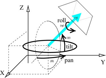
Figure 4: Camera model

Most movies are made of a large number of short elementary “shots”. Therefore, a simple model for camera motion may be adopted without losing too much expressiveness. Sophisticated camera movements are obtained by assembling sequences of shots (Refer to Christie and al.’s work [Christie et al. (2002)] for a way to perform this task). Due to a lack of space, the following description of camera movements (Figure 5) is restricted to primitive ones, and the reader is referred to the excellent book by Arijon [Arijon (1976)] for a thorough presentation of the others:

Figure 5: Camera movements

• Panoramic shot. A panoramic shot may be horizontal or vertical (i.e. around vertical or horizontal axis). The camera location is usually constant;

• Travelling (tracking shot or dolly). A general term for a camera translation;

• Zoom in or zoom out. A variation of the focal length of the camera.

To our knowledge, existing declarative camera movement generators compute camera animation frame by frame [Drucker (1994)] or use calculated key frames [Shoemake (1985)] (fixed camera location and orientation), and interpolation of the camera parameters in-between.

In contrast, the tool described here is based on a parametric representation. Computing a satisfying solution boils down to determining all the camera parameters such that some constraints on the scene are satisfied. Using the previous remark concerning simple elementary shots, parameters are modelled with degree three polynomials whose unknown is time $t$. For example, an horizontal pan (i.e. a movement along the horizontal orientation angle $\theta$) might be defined as: $\theta(t)=c_{\theta}t+d_{\theta}$, where $d_{\theta}$ represents the initial horizontal orientation of the camera (at time $t=0$) and $c_{\theta}$ is a constant velocity. Consequently, given $V_{\theta}$ the maximum allowed pan velocity, one may note that $c_{\theta}$ must lie in the domain $[-V_{\theta},V_{\theta}]$, and then $d_{\theta}$ must lie in the domain $[0,2\pi]$, in order to make any orientation starting point eligible.

In our view, the scene is considered as a problem data. Hence, from this point onward, every object composing a scene is assumed to have its location, orientation and movement already set by the user.

Object properties rely on bounding volumes (location) and object axis (orientation): each object is bounded by a volume called a bounding box. Compounds’ bounding box is the smallest box containing the bounding boxes of all the objects involved. In addition, bounding boxes may be associated to any set of objects (like a group of characters). Many geometric modellers provide such a hierarchy of bounding volumes.

The orientation of any object on the image is determined by three vectors: Front, Up and Right (Figure 6).

Figure 6: Object axis and bounding volume

6.2 Properties and Constraints

The translation of declarative descriptions of scenes into constraints is now presented. Three kinds of desired properties may be distinguished:

1. Properties on the camera;

2. Properties on the object screen location;

3. Properties on the object screen orientation.

Camera properties are a means to set constraints on the camera motion. Translation of properties on the objects of a scene is described below. The notion of frame is first introduced as an aid to constrain an object location on the screen: a frame is a rectangle whose borders are parallel to the screen borders. A frame may be inside, outside, or partially inside the screen, though it is usually fully contained in the screen. For special purposes, the frame size or/and location may be modified during the animation.

With frames, an artist can define the precise projection zone of an object from the scene (3D) to the screen (2D). Our belief in a creation helping tool leads us to prefer this kind of soft constraint to the exact 2D screen location of the projection of a 3D point.

The user defines frames (interactively or off-line), then chooses properties to apply to a frame and an object. For example, the statement (Figure 7):

“The sphere $\mathfrak{s}$ with center $(x_{\mathfrak{s}}(t),y_{\mathfrak{s}}(t),z_{\mathfrak{s}}(t))$ and radius $r$ must be fully included in the frame $\mathfrak{f}$ defined by the bottom-left point $(x^{1}_{\mathfrak{f}}(t),y^{1}_{\mathfrak{f}}(t))$ and the top-right point $(x^{2}_{\mathfrak{f}}(t),y^{2}_{\mathfrak{f}}(t))$ during the 20 seconds of the shot filmed by the camera $\mathfrak{c}$ located at $(x_{\mathfrak{c}}(t),y_{\mathfrak{c}}(t),z_{\mathfrak{c}}(t))$ with orientation $\theta_{\mathfrak{c}}(t)$ and $\phi_{\mathfrak{c}}(t)$.”

is translated into the nonlinear constraint system of equations and inequations:

$$\forall t\in[0,20]\colon\left\{\begin{array}[]{ll}x^{1}_{\mathfrak{f}}(t)&\leqslant\bigl{(}x(t)+r\bigr{)}/\bigl{(}z(t)/\gamma_{\mathfrak{c}}(t)\bigr{)}\\ x^{2}_{\mathfrak{f}}(t)&\geqslant\bigl{(}x(t)-r\bigr{)}/\bigl{(}z(t)/\gamma_{\mathfrak{c}}(t)\bigr{)}\\ y^{1}_{\mathfrak{f}}(t)&\leqslant\bigl{(}y(t)+r\bigr{)}/\bigl{(}z(t)/\gamma_{\mathfrak{c}}(t)\bigr{)}\\ y^{2}_{\mathfrak{f}}(t)&\geqslant\bigl{(}y(t)-r\bigr{)}/\bigl{(}z(t)/\gamma_{\mathfrak{c}}(t)\bigr{)}\end{array}\right.$$

with:

$$\left\{\begin{array}[]{ll}x(t)&=-\bigl{(}x_{\mathfrak{s}}(t)-x_{\mathfrak{c}}(t)\bigr{)}\sin\theta_{\mathfrak{c}}(t)+\bigl{(}y_{\mathfrak{s}}(t)-y_{\mathfrak{c}}(t)\bigr{)}\cos\theta_{\mathfrak{c}}(t)\\ y(t)&=-\bigl{(}x_{\mathfrak{s}}(t)-x_{\mathfrak{c}}(t)\bigr{)}\cos\theta_{\mathfrak{c}}(t)\sin\phi_{\mathfrak{c}}(t)+\\ &\hskip 28.45274pt\bigl{(}y_{\mathfrak{s}}(t)-y_{\mathfrak{c}}(t)\bigr{)}\sin\phi_{\mathfrak{c}}(t)\sin\theta_{\mathfrak{c}}(t)+\bigl{(}z_{\mathfrak{s}}(t)-z_{\mathfrak{c}}(t)\bigr{)}\cos\phi_{\mathfrak{c}}(t)\\ z(t)&=-\bigl{(}x_{\mathfrak{s}}(t)-x_{\mathfrak{c}}(t)\bigr{)}\cos\theta_{\mathfrak{c}}(t)\cos\phi_{\mathfrak{c}}(t)+\\ &\hskip 28.45274pt\bigl{(}y_{\mathfrak{s}}(t)-y_{\mathfrak{c}}(t)\bigr{)}\sin\theta_{\mathfrak{c}}(t)\cos\phi_{\mathfrak{c}}(t)+\bigl{(}z_{\mathfrak{s}}(t)-z_{\mathfrak{c}}(t)\bigr{)}\sin\phi_{\mathfrak{c}}(t)\end{array}\right.$$

where $\bigl{(}x(t),y(t),z(t)\bigr{)}$ is the projection of the center of $\mathfrak{s}$ in the screen space at time $t$.

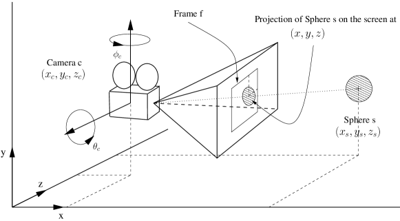
Figure 7: Projection in a frame

Note that, in order to fall back to an instance of the guaranteed tuning problem, it is possible to discard the three equations by replacing $x(t)$, $y(t)$ and $z(t)$ in the inequalities by the corresponding right-hand side.

The constraints resulting from the translation of the declarative description of “shots” contain occurrences of the universally quantified time variable $t$.

7 Examples and Benchmarking

A high-level declarative modeller tool for camera motion has been devised in order to validate the algorithms presented in Section 5. The prototype is written in C++ and Tcl/Tk; Figure 8 presents its graphical user interface: the animated scene to be filmed is displayed in a window together with the bounding volumes, while another window contains some previously drawn projection frames. The user constructs frames, selects objects, and assigns properties to objects in the scene. The output is a set of satisfying camera paths, and corresponding animations are shown in an output window.

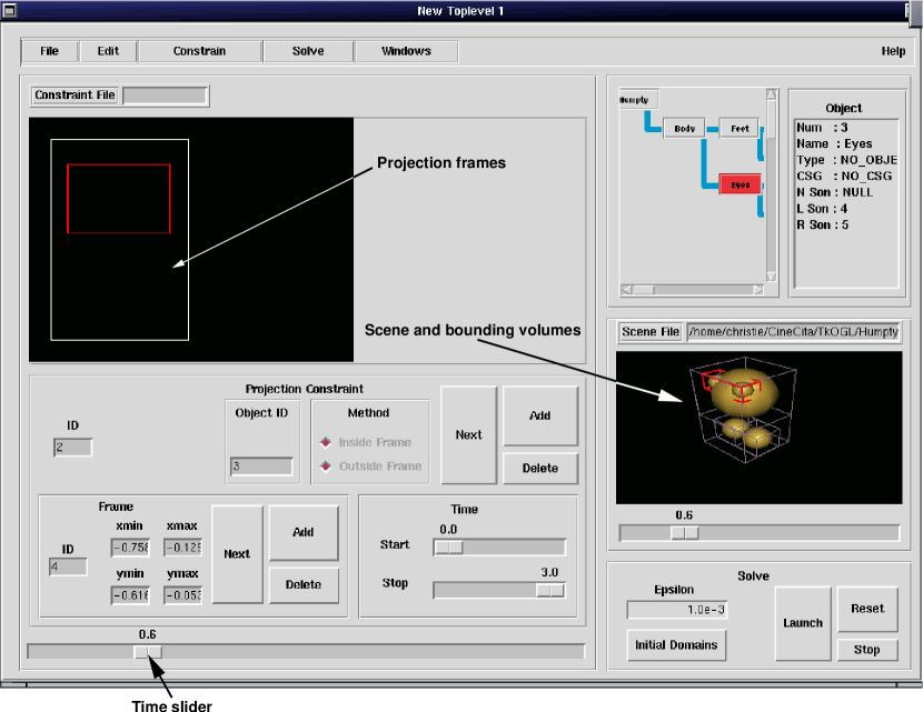
Figure 8: The declarative modeller tool

In the next section, we present some problems used to assess the quality of Alg. ${\textsf{IPA}}^{\Upsilon}$ (Tab. 5.9) using Alg. ${\textsf{ICO2}}^{{\textsf{BC3r}}}$ (Tab. 5.2 and Def. 4.5) as the inner contracting operator parameter $\Upsilon$ (hereafter referred as IPABC). Comparisons with Alg. JLA (Tab. 3) used by Jardillier and Languénou [Jardillier and Languénou (1998)] for the same kind of applications are produced and commented. Some techniques to speed-up the computation and improve the representativeness of the boxes output are also described.

7.1 Description of the benchmarks

Parabola: a curve fitting problem

This simple benchmark [Jardillier and Languénou (1998)] corresponds to finding all the parabolas lying above a given line:

$$\forall t\in[0,2]\colon at^{2}+bt+c\geqslant 2t-1\quad\text{with}\quad a\in[0,1],b\in[0,1],c\in[0,1]$$

Circle: a trivial collision problem

Benchmark Circle is a collision problem: given $B$ a point moving along a circling path, find all points $A$ such that the distance between $A$ and $B$ is always greater than a given value. Benchmarks Circle₂ and Circle₃ are instances of the same problem with respectively $2$ and $3$ points moving round in circles. For only one circling point, we have:

$$\begin{array}[]{l}\forall t\in[-\pi,\pi]\colon\\[2.0pt] \hskip 15.0pt\sqrt{(r_{1}\sin t-x)^{2}+(r_{1}\cos t-y)^{2}}\geqslant d_{1}\end{array}\quad\text{with}\quad\left\{\begin{array}[]{l}x\in[-5,5]\\ y\in[-5,5]\\ d_{1}=0.5\\ \end{array}\right.$$

where $d_{1}$ is the mandatory minimal distance between $A$ and $B$, and $r_{1}=2.5$ is the radius of $B$’s circling path.

Satellite: a collision problem

Given $n$ satellites swivelling around a planet (Figure 9), we are looking for the parameters of an $(n+1)$th trajectory on which to put another satellite. Obviously, this trajectory must be such that the added satellite never collides with the already launched ones.

The position of the $i$th satellite at time $t$ is defined by:

$$\mathbf{f_{i}}(t)=\left(\begin{array}[]{l}x_{i}(t)\\ y_{i}(t)\\ z_{i}(t)\\ \end{array}\right)=\left(\begin{array}[]{l}d_{i}\cos{\theta_{i}}\sin{\omega_{i}t+\phi_{i}}\\ d_{i}\bigl{(}\sin{\psi_{i}}\sin{\theta_{i}}\sin{(\omega_{i}t+\phi_{i})}+\cos{\psi_{i}}\cos{(\omega_{i}t+\phi_{i})}\bigr{)}\\ d_{i}\bigl{(}-\cos{\psi_{i}}\sin{\theta_{i}}\sin{(\omega_{i}t+\phi_{i})}+\sin{\psi_{i}}\cos{(\omega_{i}t+\phi_{i})}\bigr{)}\end{array}\right)$$

where variables $\theta_{i}$ and $\phi_{i}$ define the orientation of the plane of revolution, $\omega_{i}$ the angular velocity of the satellite and $\phi_{i}$ its initial position at $t=0$. Variable $d_{i}$ stands for the radius of the circle of revolution. Considering $n$ satellites, we are looking for consistent values of the unknowns $\theta_{j},\phi_{j},\omega_{j},d_{j}$ of the satellite $j=n+1$ such that:

$$\forall t\in[-\pi,\pi]\colon\left\{\begin{array}[]{l}{\textsf{dist}}\bigl{(}\mathbf{f_{1}}(t),\mathbf{f_{j}}(t)\bigr{)}\geqslant s\\ {\textsf{dist}}\bigl{(}\mathbf{f_{2}}(t),\mathbf{f_{j}}(t)\bigr{)}\geqslant s\\ \vdots\\ {\textsf{dist}}\bigl{(}\mathbf{f_{n}}(t),\mathbf{f_{j}}(t)\bigr{)}\geqslant s\end{array}\right.$$

where $s$ represents the minimal distance allowed between two satellites.

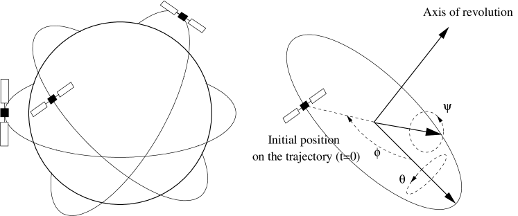
Figure 9: A collision-free problem

The unknowns to be computed are $\theta_{j},\phi_{j}$ and $\psi_{j}$, with domains $[0,2\pi]$. In this benchmark, we consider three satellites in the air with the following parameters:

Parameter	Satellite 1	Satellite 2	Satellite 3
$d_{i}$	5.0	5.0	5.0
$\omega_{i}$	1.0	1.0	1.0
$\phi_{i}$	0.0	1.0	2.0
$\theta_{i}$	0.0	1.0	1.5
$\psi_{i}$	0.0	1.0	1.5

Robot: a collision problem

This benchmark is based on Example 1.1, p. 1.1. The actual constraint system to solve is:

$$\forall t\in[0,2]\colon\sqrt{\bigl{(}x-P_{x}(t)\bigr{)}^{2}+\bigl{(}y-P_{y}(t)\bigr{)}^{2}}\geqslant d$$

where

$$\left\{\begin{array}[]{l}P_{x}(t)=d_{1}\sin\alpha_{1}(t)+d_{2}\sin\bigl{(}\alpha_{1}(t)+\alpha_{2}(t)-\pi\bigr{)}+d_{3}\sin\bigl{(}\alpha_{1}(t)+\alpha_{2}(t)+\alpha_{3}(t)\bigr{)}\\ P_{y}(t)=d_{1}\cos\alpha_{1}(t)+d_{2}\cos\bigl{(}\alpha_{1}(t)+\alpha_{2}(t)-\pi\bigr{)}+d_{3}\cos\bigl{(}\alpha_{1}(t)+\alpha_{2}(t)+\alpha_{3}(t)\bigr{)}\\ \alpha_{1}(t)=t+\pi/4\\ \alpha_{2}(t)=2t-1\\ \alpha_{3}(t)=0.2t+0.1\end{array}\right.$$

The initial domains for the unknowns $x$ and $y$ are both set to $[0,5]$, the size of the robot’s hand is set to $0.5$ and the respective lengths of the arm’s segments are $d_{1}=1.0$, $d_{2}=2.0$ and $d_{3}=1.0$.

PointPath: a motion planning problem

This benchmark [Jaulin and Walter (1996)] introduces a simple motion planning problem (Figure 10). We need to compute an object’s path, starting at position $M_{0}$ and ending at position $M_{1}$, while avoiding collision with the ground and some objects. The path $M(t)$ is tentatively chosen as a polynomial written as a linear combination of Bernstein polynomials of degree 3, and controlled by the points $P_{1}$ and $P_{2}$ of unknown coordinates:

$$M(t)=M_{0}B^{3}_{0}(t)+P_{1}B^{3}_{1}(t)+P_{2}B^{3}_{2}(t)+M_{1}B^{3}_{3}(t)$$

where the Bernstein polynomials are:

$$B^{3}_{0}(t)=(1-t)^{3},\>B^{3}_{1}(t)=3t(1-t)^{2},\>B^{3}_{2}(t)=3t^{2}(1-t),\>B^{3}_{3}=t^{3}$$

The constraints specify that for all $t$ in the time frame:

1. $M(t)$ must be above a curve representing the floor;

2. the distance between $M(t)$ and a static object $S=(4.8,1.0)$ must be greater than $1$.

Which leads to:

$$\forall t\in[0,1]\colon\left\{\begin{array}[]{l}\bigl{(}x(t)-4.8\bigr{)}^{2}+\bigl{(}y(t)-1\bigr{)}^{2}\geqslant 1\\ y(t)\geqslant\sin\bigl{(}x(t)\bigr{)}\\ \end{array}\right.$$

with $M(t)=\displaystyle\binom{x(t)}{y(t)}$. Domains for the coordinates of $P_{1}$ and $P_{2}$ are initialized to $[-10,10]$.

Figure 10: Solution for the motion-planning problem

Projection: a camera control problem

Benchmark Projection corresponds to the problem of projecting a moving sphere in a moving frame, already presented in Section 6.2. The initial values chosen for the camera are the following: $x_{c}\in[-3,3]$, $y_{c}\in[-3,3]$, $z_{c}=2$, $\phi_{c}\in[-0.5,0.5]$, $\theta_{c}=0$, and $\gamma_{c}=0.8$.

Projection₄ is the original problem presented in Section 6.2; Projection₅ is the same problem with one more constraint on the distance between the sphere and the camera; Projection₈ is the problem with two frames and two spheres.

GarloffGraf1: inner approximation computation [Garloff and Graf (1999)]

Find the values for the parameters $v$ and $w$ ensuring the stability of the polynomial:

$$p(s)=s^{3}+vs^{2}+(w-5v-13)s+w$$

Using the Linard-Chipart criterion, the problem can be transformed into the equivalent system:

$$v,w >0$$

$$-5v^{2}-13v+vw-w >0$$

Following Garloff and Graf, we compute the inner approximation of the relation $-5v^{2}-13v+vw-w>0$ for $v\in[2,10]$ and $w\in[40,50]$.

GarloffGraf2: inner approximation computation [Garloff and Graf (1999)]

This is again a stability problem: find sound values for $A$, $B$, and $D$ verifying:

$$A,B,D >0$$

$$AB^{2}-D^{2} >0$$

$$-AB+A+D^{2}-D-1 >0$$

$$AB-AD-2A+D^{3}+4D^{2}+4D >0$$

$$AB^{3}-AB^{2}D-4AB^{2}+2ABD+4AB+2BD^{3}+5BD^{2}+2BD-D^{3}-4D^{2}-4D >0$$

$$AB-2A-BD^{2}-4BD-4B-2D^{2}+3D-2 >0$$

Following Garloff and Graf, the initial domains chosen are $A\in[100,120]$, $B\in[0,2]$, and $D\in[10,20]$.

According to Abdallah and al. [Abdallah et al. (1996)], a CAD-based software such as QEPCAD (http://www.cs.usna.edu/~qepcad/B/QEPCAD.html) requires more than two hours to prove the existence of a solution to the problem.

7.2 Improving Computation

Solvers such as Numerica usually isolate solutions with variable domains around $10^{-8}$ or $10^{-16}$ in width. By contrast, the applications this paper focuses on are less demanding since the resulting variable domains are used in the context of a display screen, a “low resolution” device. In practice, one can consider that a reasonable threshold $\varepsilon$ for the splitting process during the search is some value lower or equal to $10^{-2}$ or $10^{-3}$.

One of the drawbacks of Algorithm JLA [Jardillier and Languénou (1998)] is that successive output solutions are very similar, while it is of importance to be able to provide the user with a representative sample of solutions as soon as possible. Tackling this problem using Alg. IPABC is done as follows: given a constraint system of the form $\forall t\in I_{t}\colon c_{1}\wedge\cdots\wedge c_{m}$ and a Cartesian product of domains $\mathbf{B}=I_{1}\times\cdots\times I_{n}$, we have two degrees of freedom during the solving process, viz. the selection of the next constraint to consider, and the selection of the next variable to split. Figure 11 presents the differences with regard to the order of generation of solutions for Circle₂ for two strategies concerning the variable splitting order:

• depth-first, where each constraint is considered in turn, and each domain is split to the threshold splitting limit;

• semi-depth-first where each constraint is considered in turn, but each variable is split only once and then put at the end of the domain queue.

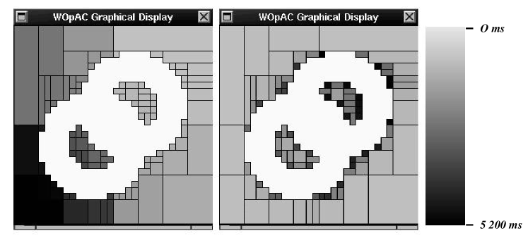
Figure 11: Depth-first vs. semi-depth-first

As one may see, the semi-depth-first algorithm computes consecutive solutions spread over all the search space, while the depth-first algorithm computes solutions downward and from right to left.

Some strategies on constraint consideration order have also been investigated, whose impact on speed is described hereunder. Four strategies may be singled out:

Simple method

Box consistency is applied on the negation of each constraint in turn;

Pre-parse method

This method interleaves the simple method with a pre-parse algorithm: given a constraint $c$, and $t$ the universally quantified variable, $k$ canonical intervals are extracted from the domain $I_{t}$ of $t$, and the consistency of $c$ is tested for every one of them. At this stage, a failed check is sufficient to initiate a backtrack;

Normal method

Box consistency is computed both for each constraint and for its negation;

Global method

Given constraints $c_{i},c_{i+1},\dots,c_{m}$, the global method applies the normal method on $c_{i}$, then checks whether the output boxes are consistent with the remaining constraints by mere evaluation.

Charts in Figure 12 present the time spent for obtaining the first and all solutions for four benchmarks on a SUN UltraSparc 1/167 MHz under Solaris 2.5.

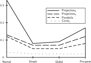
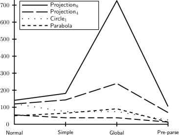
A.  B.

Figure 12: A) First solution. B) All solutions (times in seconds)

Considering first Chart A, one may see that the simple method is the most interesting strategy for computing the first solution, while the normal method is very time consuming for problems with “many” constraints (projection₈). On the other hand, while the pre-parse method is a bad choice for computing only one solution, it is competitive for obtaining all solutions.

7.3 Results

Algorithms JLA and IPABC provide different sets of solutions for the same problem. Consequently, a direct comparison of their performances is quite difficult. Moreover, the actual implementation of JLA uses a splitting threshold $\omega$ for slicing the domain of the universally quantified variable $t$ instead of checking consistency by eventually reaching canonicity of the samples of the domain $I_{t}$. Figure 13 shows the impact of the threshold on the computed solutions for benchmark Circle₂.

Figure 13: Impact of the time splitting threshold $\omega$ on precision in JLA (from left to right: $\omega=0.5$, $\omega=0.1$, and $\omega=0.05$)

Table 13 (resp. 13) compares algorithms JLA and IPABC from the speed point of view for computing the first solution (resp. all solutions). Times are given in seconds on a Pentium III at 800 MHz under Linux.

Benchmark	JLA	IPABC	JLA/IPABC
Parabola $(\varepsilon=10^{-2})$	0.04	0.02	2.0
Parabola $(\varepsilon=10^{-3})$	0.77	0.02	38.5
Circle2 $(\varepsilon=10^{-2})$	3.52	0.01	352000
Circle2 $(\varepsilon=10^{-3})$	3.57	0.01	357000
Satellite $(\varepsilon=10^{-2})$	0.91	0.99	0.91
Satellite $(\varepsilon=10^{-3})$	68.7	0.99	68.48
Robot $(\varepsilon=10^{-1})$	0.13	0.01	13
Robot $(\varepsilon=10^{-2})$	0.50	0.01	50
Projection8 $(\varepsilon=10^{-1})$	0.05	0.07	0.71
Projection8 $(\varepsilon=10^{-2})$	0.14	0.07	2.0
Projection8 $(\varepsilon=10^{-3})$	3.01	0.07	43.0
Projection4 $(\varepsilon=10^{-2})$	0.11	0.03	3.66
Projection4 $(\varepsilon=10^{-3})$	1.11	0.03	37
GarloffGraf1 $(\varepsilon=10^{-2})$	15.79	0.01	1579
GarloffGraf2 $(\varepsilon=10^{-2})$	5.58	0.04	139
PointPath $(\varepsilon=0.5)$	???	7.85	???

JLA vs. IPABC—First solution

As one can see, the efficiency of IPABC compared to the one of JLA increases steadily with the precision required.

We were not able to obtain any result for PointPath with JLA after several hours.

Benchmark	JLA	IPABC	JLA/IPABC
Parabola	10.65	1.22	8.72
Circle2	3.16	0.15	21.06
Circle3	3.41	0.55	6.2
Satellite	$>$600	54.91	$>$ 175
Robot	22.65	1.97	11.5
Projection8	$>$600.00	3.43	$>$175.4
Projection5	182.09	16.01	11.35
GarloffGraf1 $(\varepsilon=10^{-2})$	422.54	1.49	283.6
GarloffGraf2 $(\varepsilon=10^{-2})$	29.54	1.04	28.40
PointPath $(\varepsilon=0.5)$	???	534.14	???

JLA vs. IPABC—All solutions

8 Conclusion

Unlike the methods used to deal with universally quantified variables described in [Hong and Buchberger (1991)], the algorithms presented in this paper are purely numerical ones (except for the negation of constraints). Since they rely on “traditional” techniques used by most of the interval constraint-based solvers, they may benefit from the active researches led to speed up these tools. What is more, they are applicable to the large range of constraints for which an outer contracting operator may be devised. By contrast, CAD-based methods deal with polynomial constraints only, as is the case with the method based on Bernstein expansion [Garloff and Graf (1999)].

Despite the dramatic improvement of the new method described herein over the one given by Jardillier and Languénou, handling of complex scenes with many objects and a camera allowed to move along all its degrees of freedom in a reasonable time is beyond reach for the moment. Nevertheless, a comforting idea is that most of the traditional camera movements involve but few of the degrees of freedom, thereby reducing the number of variables to consider.

Following the work of Markov [Markov (1995)] and Shary [Shary (1995)], a direction for future research is to compare the use of Kaucher arithmetic [Kaucher (1980)] to compute inner approximations of relations with the use of outer contracting operators. Their work is also related to the one by Armengol et al. [Armengol et al. (1998)] and Gardeñes et al. [Gardeñes and Trepat (1980), Gardeñes and Mielgo (1986)] on modal interval arithmetic. Yet, these approaches require algebraizing trigonometric constraints, an operation known to slow down computation [Pau and Schicho (2000)].

APPENDIX

Appendix A Notations

$\mathbb{F}$	Set of floating-point numbers
${a}^{+}$	Smallest floating-point number greater than $a$
${a}^{-}$	Greatest floating-point number smaller than $a$
$\mathbb{I}$	Set of closed intervals whose bounds are floating-point numbers
${\textsf{Outer}}(\rho)$	Smallest box containing $\rho$: ${\textsf{Outer}}(\rho)=\bigcap\{\mathbf{B}\in\mathbb{I}^{n}\mid\rho\subseteq\mathbf{B}\}$
${\textsf{Inner}}(\rho)$	Inner approximation of $\rho$:
	${\textsf{Inner}}(\rho)=\{\mathbf{r}\in\mathbb{R}^{n}\mid{\textsf{Outer}}(\{\mathbf{r}\})\subseteq\rho\}$
$\Lbag{\mathcal{S}}\Rbag$	Union of the boxes in $\mathcal{S}$:
	$\Lbag{\{\mathbf{B_{1}},\dots,\mathbf{B_{n}}\}}\Rbag=\{\mathbf{r}\in\mathbb{R}^{n}\mid\exists i\in\{1,\dots,n\}\text{ s.t. }\mathbf{r}\in\mathbf{B_{i}}\}$
$\rho_{c}$	Relation associated to the constraint $c$:
	$\rho_{c}=\{(r_{1},\dots,r_{n})\in\mathbb{R}^{n}\mid c(r_{1},\dots,r_{n})\}$
$\rho_{c^{\forall}}$	Relation associated to $\forall v\in I:c$
$\overline{c}$	“Negation” of the constraint $c$: ($\overline{f\leqslant 0}$ is defined as $f\geqslant 0$)
${\textsf{Dom}}_{\mathbf{B}}(x)$	Domain of the variable $x$ in the box $\mathbf{B}$
$\mathbf{B_{1}}\boxbslash\mathbf{B_{2}}$	Set difference of $\mathbf{B_{1}}$ and $\mathbf{B_{2}}$ as a set of boxes:
	$\Lbag{\mathbf{B_{1}}\boxbslash\mathbf{B_{2}}}\Rbag=\{r\in\mathbf{B_{1}}\mid{\textsf{Outer}}(\{r\})\cap\mathbf{B_{2}}=\varnothing\}$
$\mathbf{B}_{{I}\mathbin{\leftarrow}{J}}$	Box $\mathbf{B}$ where the interval $I$ is replaced by the interval $J$
$\mathcal{P}(\mathcal{S})$	Power set of the set $\mathcal{S}$
${\textsf{Split}}_{k}(\mathbf{B})$	Split in $k$ boxes the box $\mathbf{B}$
${\textsf{Split}}^{\setminus v}_{k}(\mathbf{B})$	Split in $k$ boxes the box $\mathbf{B}$ (never splits the interval corresponding to the
	domain of $v$
$\displaystyle\biguplus_{i}\{(\mathcal{U}_{1},\dots,\mathcal{U}_{n})\}$	union of vectors of sets componentwise:
	$\displaystyle\biguplus_{i}\{(\mathcal{U}_{1}^{i},\dots,\mathcal{U}_{n}^{i})\}=(\displaystyle\bigcup_{i}\mathcal{U}_{1}^{i},\dots,\allowbreak\displaystyle\bigcup_{i}\mathcal{U}_{n}^{i})$

The authors gratefully acknowledge the insightful perusal of the anonymous referees and discussions with Laurent Granvilliers and Lucas Bordeaux that helped improve preliminary versions of this paper.

eceived July 2000; revised September 2002; accepted May 2003

References

- Abdallah et al. (1996) Abdallah, C., Dorato, P., Yang, W., Liska, R., and Steinberg, S. 1996. Applications of quantifier elimination theory to control theory. In Proceedings of the 4th IEEE Mediterranean Symposium on Control and Automation. Malene, Crete, Greece, 340–345.
- Abrams and Allen (1997) Abrams, S. and Allen, P. K. 1997. Computing camera viewpoints in an active robot work-cell. Tech. Rep. IBM Research Report: RC 20987, IBM Research Division.
- Alefeld and Herzberger (1983) Alefeld, G. and Herzberger, J. 1983. Introduction to Interval Computations. Academic Press Inc., New York, USA.
- Arijon (1976) Arijon, D. 1976. Grammar of the film language. Hastings House Publishers.
- Armengol et al. (1998) Armengol, J., Travé-Massuyès, L., Vehí, J., and Sáinz, M. A. 1998. Modal interval analysis for error-bounded semiqualitative simulation. In 1r Congrés Català d’Intelligència Artificial. 223–231.
- Benhamou (1995) Benhamou, F. 1995. Interval constraint logic programming. In Constraint programming: basics and trends: 1994 Châtillon Spring School, Châtillon-sur-Seine, France, May 16–20, 1994, A. Podelski, Ed. Lecture notes in computer science, vol. 910. Springer-Verlag, 1–21.
- Benhamou (1996) Benhamou, F. 1996. Heterogeneous constraint solving. In Procs. of the 5th International Conference on Algebraic and Logic Programming (ALP’96), LNCS 1139. Springer-Verlag, Aachen, Germany, 62–76.
- Benhamou et al. (1999) Benhamou, F., Goualard, F., Granvilliers, L., and Puget, J.-F. 1999. Revising hull and box consistency. In Procs. of the 16th Int. Conf. on Logic Programming (ICLP’99). The MIT Press, Las Cruces, USA, 230–244. ISBN 0-262-54104-1.
- Benhamou et al. (1994) Benhamou, F., McAllester, D., and Van Hentenryck, P. 1994. CLP(Intervals) revisited. In Procs. of the International Symposium on Logic Programming (ILPS’94). MIT Press, Ithaca, NY, 124–138.
- Benhamou and Older (1997) Benhamou, F. and Older, W. J. 1997. Applying interval arithmetic to real, integer and boolean constraints. Journal of Logic Programming 32, 1, 1–24.
- Blinn (1988) Blinn, J. 1988. Where am I? what am I looking at? IEEE Computer Graphics and Applications 8, 4 (July), 76–81.
- Christie et al. (2002) Christie, M., Languénou, E., and Granvilliers, L. 2002. Modeling Camera Control with Constrained Hypertubes. In Proceedings of the International Conference on Principles and Practice of Constraint Programming (CP’2002), P. V. Hentenryck, Ed. LNCS, vol. 2470. Springer-Verlag, 618–632.
- Collavizza et al. (1999) Collavizza, H., Delobel, F., and Rueher, M. 1999. Extending consistent domains of numeric CSP. In Procs. of the 16th IJCAI. Vol. 1. Stockholm, Sweden, 406–411.
- Collins (1975) Collins, G. E. 1975. Quantifier elimination for real closed fields by cylindrical algebraic decomposition. In Procs. of the 2nd GI Conf. Automata Theory and Formal Languages. Lecture Notes in Computer Science, vol. 33. Springer, Kaiserslauten, 134–183.
- Davenport et al. (1991) Davenport, G., Smith, T. A., and Pincever, N. 1991. Cinematic primitives for multimedia. IEEE Computer Graphics and Applications 11, 4 (July), 67–74.
- Drucker (1994) Drucker, S. M. 1994. Intelligent camera control for graphical environments. Ph.D. thesis, Massachusetts Institute of Technology, Program in Media Arts and Sciences, School of Architecture and Planning.
- Drucker et al. (1992) Drucker, S. M., Galyean, T. A., and Zeltzer, D. 1992. CINEMA: A system for procedural camera movements. In Procs. of the 1992 Symposium on Interactive 3D Graphics, M. Levoy and E. E. Catmull, Eds. ACM Press, Cambridge, MA, 67–70.
- Drucker and Zeltzer (1994) Drucker, S. M. and Zeltzer, D. 1994. Intelligent camera control in a virtual environment. In Procs. of Graphics Interface ’94. Canadian Information Processing Society, Banff, Alberta, Canada, 190–199.
- Ebers and Moll (1954) Ebers, J. J. and Moll, J. L. 1954. Large-scale behaviour of junction transistors. IRE Procs. 42, 1761–1772.
- Emiris and Mourrain (1999) Emiris, I. Z. and Mourrain, B. 1999. Computer algebra methods for studying and computing molecular conformations. Algorithmica 25, 2/3, 372–402.
- Farouki and Rajan (1987) Farouki, R. T. and Rajan, V. T. 1987. On the numerical condition of polynomials in Bernstein form. Computer Aided Geometric Design 4, 191–216.
- Gardeñes and Trepat (1980) Gardeñes, E. and Trepat, A. 1980. Fundamentals of SIGLA, an interval computing system over the completed set of intervals. Computing 24, 2–3, 161–179.
- Gardeñes and Mielgo (1986) Gardeñes, E. H. and Mielgo, H. 1986. Modal intervals: reasons and ground semantics. In Interval Mathematics. Number 212 in Lecture Notes in Computer Science. Springer-Verlag.
- Garloff and Graf (1999) Garloff, J. and Graf, B. 1999. Solving strict polynomial inequalities by Bernstein expansion. In The Use of Symbolic Methods in Control System Analysis and Design, N. Munro, Ed. The Institution of Electrical Engineers, London, England, 339–352.
- Gleicher and Witkin (1992) Gleicher, M. and Witkin, A. 1992. Through-the-lens camera control. In Computer Graphics (SIGGRAPH ’92 Proceedings), E. E. Catmull, Ed. Vol. 26-2. 331–340.
- Granvilliers and Benhamou (2001) Granvilliers, L. and Benhamou, F. 2001. Progress in the solving of a circuit design problem. Journal of Global Optimization 20, 2, 155–168.
- Hansen (1992) Hansen, E. R. 1992. Global Optimization Using Interval Analysis. Pure and Applied Mathematics. Marcel Dekker Inc.
- Haroud and Faltings (1994) Haroud, D. and Faltings, B. 1994. Global consistency for continuous constraints. Lecture Notes in Computer Science 874, 40–50.
- Hong and Buchberger (1991) Hong, H. and Buchberger, B. 1991. Speeding-up quantifier elimination by Gröbner bases. Technical Report 91-06, RISC-Linz, Johannes Kepler University, Linz, Austria.
- IEEE (1985) IEEE. 1985. IEEE standard for binary floating-point arithmetic. Tech. Rep. IEEE Std 754-1985, Institute of Electrical and Electronics Engineers. Reaffirmed 1990.
- Jardillier and Languénou (1998) Jardillier, F. and Languénou, É. 1998. Screen-space constraints for camera movements: the virtual cameraman. In Eurographics’98 proceedings, N. Ferreira and M. Göbel, Eds. Vol. 17. Blackwell Publishers, 108 Cowley Road, Oxford OX4 IJF, UK, 175–186.
- Jaulin and Walter (1993) Jaulin, L. and Walter, E. 1993. Set inversion via interval analysis for nonlinear bounded-error estimation. Automatica 29, 4, 1053–1064.
- Jaulin and Walter (1996) Jaulin, L. and Walter, E. 1996. Guaranteed tuning with application to robust control and motion planning. Automatica 32, 8, 1217–1221.
- Jirstrand (1995) Jirstrand, M. 1995. Cylindrical algebraic decomposition—an introduction. Technical Report 1995-10-18, Department of Electrical Engineering, Linköping University, Sweden.
- Kaucher (1980) Kaucher, E. W. 1980. Interval analysis in the extended interval space . Computing. Supplementum 2, 33–49.
- Kutsia and Schicho (1999) Kutsia, T. and Schicho, J. 1999. Numerical solving of constraints of multivariate polynomial strict inequalities. Technical report 99-31, RISC Institute.
- Lefèvre et al. (1998) Lefèvre, V., Muller, J.-M., and Tisserand, A. 1998. The table maker’s dilemma. IEEE Transactions on Computers 47, 11 (Nov.).
- Mackworth (1977) Mackworth, A. K. 1977. Consistency in networks of relations. Artificial Intelligence 1, 8, 99–118.
- Markov (1995) Markov, S. 1995. On directed interval arithmetic and its applications. Journal of Universal Computer Science 1, 7, 514–526.
- Meintjes and Morgan (1990) Meintjes, K. and Morgan, A. P. 1990. Chemical equilibrium systems as numerical test problems. ACM Trans. Math. Softw. 16, 2 (June), 143–151.
- Moore (1966) Moore, R. E. 1966. Interval Analysis. Prentice-Hall, Englewood Cliffs, N.J.
- Neumaier (1990) Neumaier, A. 1990. Interval methods for systems of equations. Encyclopedia of Mathematics and its Applications, vol. 37. Cambridge Unversity Press.
- Older and Vellino (1990) Older, W. J. and Vellino, A. 1990. Extending Prolog with constraint arithmetic on real intervals. In Proc. of IEEE Canadian conference on Electrical and Computer Engineering. IEEE Computer Society Press, New York.
- Pau and Schicho (2000) Pau, P. and Schicho, J. 2000. Quantifier elimination for trigonometric polynomials by cylindrical trigonometric decomposition. Journal of Symbolic Computation 29, 6 (June).
- Puget (1994) Puget, J.-F. 1994. A C++ implementation of CLP. In Procs. of the Singapore Conference on Intelligent Systems (SPICIS’94). Singapore.
- Puget and Van Hentenryck (1998) Puget, J.-F. and Van Hentenryck, P. 1998. A constraint satisfaction approach to a circuit design problem. Journal of Global Optimization 13, 75–93.
- Rademacher (1948) Rademacher, H. A. 1948. On the accumulation of errors in processes of integration on high-speed calculating machines. Annals Comput. Laor. Harvard Univ. 16, 176–185. Cited in Stoer and Bulirsch (1993).
- Sam (1995) Sam, J. 1995. Constraint consistency techniques for continuous domains. Ph.D. thesis, École polytechnique fédérale de Lausanne.
- Shary (1995) Shary, S. P. 1995. Algebraic solutions to interval linear equations and their applications. In Numerical Methods and Error Bounds, proceedings of the IMACS-GAMM International Symposium on Numerical Methods and Error Bounds, G. Alefeld and J. Herzberger, Eds. Berlin, Akademie Verlag, Oldenburg, Germany, 224–233.
- Shary (1999) Shary, S. P. 1999. Interval Gauss-Seidel method for generalized solution sets to interval linear systems. In MISC’99 — Workshop on Applications of Interval Analysis to Systems and Control. Girona, Spain, 51–65.
- Shoemake (1985) Shoemake, K. 1985. Animation rotations with quaternion curves. Computer Graphics 19, 3, 245–254. Procs. of SIGGRAPH’85, San Francisco, CA.
- Snyder (1992) Snyder, J. M. 1992. Interval analysis for computer graphics. In Computer Graphics (SIGGRAPH ’92 Proceedings), E. E. Catmull, Ed. Vol. 26-2. 121–130.
- Stoer and Bulirsch (1993) Stoer, J. and Bulirsch, R. 1993. Introduction to Numerical Analysis, second ed. Number 12 in Texts in Applied Mathematics. Springer, Heidelberg.
- Sunaga (1958) Sunaga, T. 1958. Theory of an interval algebra and its application to numerical analysis. In Research Association of Applied Geometry Memoirs of the unifying study of basic problems in engineering and physical sciences by means of geometry, K. Kondo, Ed. Vol. 2. Gakujutsu Bunken Fukyu-Kai, Japan, Chapter Miscellaneous Subjects II, 547–564.
- Tarabanis (1990) Tarabanis, K. 1990. Automated sensor planning and modeling for robotic vision tasks. Tech. Rep. CUCS-045-90, University of Columbia.
- Turing (1948) Turing, A. M. 1948. Rounding-off errors in matrix processes. Quart. J. Mech. 1, 287–308. Cited in Wilkinson (1963).
- Van Hentenryck et al. (1997) Van Hentenryck, P., McAllester, D., and Kapur, D. 1997. Solving polynomial systems using a branch and prune approach. SIAM Journal on Numerical Analysis 34, 2 (Apr.), 797–827.
- Van Hentenryck et al. (1997) Van Hentenryck, P., Michel, L., and Deville, Y. 1997. Numerica: A Modeling Language for Global Optimization. The MIT Press.
- Waltz (1975) Waltz, D. L. 1975. Understanding line drawings of scenes with shadows. In The Psychology of Computer Vision, P. H. Winston, B. Horn, M. Minsky, and Y. Shirai, Eds. McGraw-Hill, New York, Chapter 2, 19–91.
- Ward et al. (1989) Ward, A. C., Lozano-Pérez, T., and Seering, W. P. 1989. Extending the constraint propagation of intervals. In Procs. of IJCAI’89. 1453–1458.
- Wilkinson (1963) Wilkinson, J. H. 1963. Rounding errors in algebraic processes. Prentice-Hall, New Jersey. Reprinted as Dover Publications (1994).