EXPLOITING DIVERSITY
FOR NATURAL LANGUAGE PARSING

Abstract

Accurate linguistic annotation is a core requirement of natural language processing systems. The demand for accuracy in the face of rapid prototyping constraints and numerous target languages has led to the employment of machine learning methods for developing linguistic annotation systems.

The popularity of applying machine learning methods to computational linguistics problems has given rise to a large supply of trainable natural language processing systems. Most problems of interest have an array of off-the-shelf products or downloadable code implementing solutions using various techniques. In situations where these solutions are developed independently, it is observed that their errors tend to be independently distributed. In this thesis we discuss approaches for capitalizing on this situation in a sample problem domain, Penn Treebank-style parsing.

The machine learning community provides us with techniques for combining outputs of classifiers, but parser output is more structured and interdependent than classifications. To overcome this, two novel strategies for combining parsers are used: learning to control a switch between parsers and constructing a hybrid parse from multiple parsers’ outputs. In this thesis we give supervised and unsupervised techniques for each of these strategies as well as performance and robustness results from evaluation of the techniques.

One shortcoming of combining off-the-shelf parsers is that the parsers are not developed with the intention to perform well on complementary data or to compensate for each others’ weaknesses. The individual parsers are globally optimized. We present two techniques for producing an ensemble of parsers in such a way that their outputs can be constructively combined. All of the ensemble members will be created using the same underlying parser induction algorithm, and the method for producing complementary parsers is only loosely coupled to that algorithm.

Dedicated to
good parents,
Kathleen and Daniel

No one flourishes in isolation and I am another example to support the claim. There are many people I should thank, and tracing back all of the paths of inspiration, motivation, and support that facilitate a thesis is impossible. Here is an overview of the major supporting members of the cast:

My readers, Steven Salzberg and David Yarowsky, have given me very useful suggestions and comments about my thesis research. They have each contributed immensely to my education.

My friends at Hopkins have given me plenty of arguments and feedback concerning this thesis and other things, and I especially thank them for tolerating my discussions concerning ground beef superhighways and antiseptic qualities of Diet Coke. I was always in good company at Hopkins.

My advisor, Eric Brill, provided me with both the liberty to pursue research that I found interesting, and the constraints I required to complete my thesis research. He made me feel valuable to the Hopkins NLP lab and the larger research community without treating me as just another information worker. I could not have asked for a better advisor.

My parents gifted me with a love of learning by teaching me through play and letting me disassemble most household items. All along, my entire family prepared me to pursue research.

Katya, my beloved wife, has developed a capacity for patience that I would have never believed possible. Her love and support have eased many desperate moments in my graduate career. Without her encouragement, my days would have been dim and my nights dismal.

Chapter 1 Corpus-based Natural Language Processing

Computers do not understand human languages. They can store and search instances of linguistic data, as long as the search keys are patterns which are very simple and similar to the data. In this respect, though, they are no more than advanced books or tape recorders. The massive quantity of human knowledge can be preserved in this way, but not extended. It can be inspected, but not summarized.

The accelerating growth of the quantity of knowledge possessed by the human race has been of concern for more than half a century [19]. The concern has been whether our archival media can keep pace with that rate of growth. At this point, however, it appears that the problem is understood and solvable with current tools. The World Wide Web has quickly become the de facto repository for knowledge.

A problem of equal concern has been looming over the horizon, and did not require our attention until its predecessor was solved. At some point in our future the temporally finite nature of human life will restrict what inferences can be made from the wealth of knowledge. The time will come when adding a piece of scientific knowledge via deduction or experimentation will require more examination of the repository of knowledge, and more time spent in deduction and experimentation than a single human has the ability to give.

Whether humans can develop a social system for passing incomplete deductions for others to continue is an open question. At this point it seems plausible that every deduction that has been made can be attributed to some individual.

We have just presented two motivating reasons for producing systems that are able to understand human languages, in the guise of a single reason. To clarify:

• Computers that understand language can better search through and summarize the existing wealth of human knowledge.

• Artifacts with the ability to inference about concepts expressible in human languages can be given arbitrarily long lifetimes. They will be able to make additions to the repository of human knowledge without restriction. In the near term, they will be able to double-check the repository for consistency, validate new scientific claims, and suggest lines of research that have not yet been explored.

The problem of reasoning about natural language concepts is far beyond the scope of a thesis. The CYC project attempted to solve this problem in only eleven years starting in 1984, and they continue to work on it today [63]. The computational linguistics and natural language processing community is attempting to move toward the solution to this problem by modeling progressively more complex linguistic phenomena. The high-level goal is to produce a model that can infer underlying semantics given only surface realizations, the observable pieces of a language.

There are many techniques that have been used to build these models. Many people (probably every budding computer scientist) have tried to build these systems by hand using introspection as their guide. Repeated experimentation has shown us that with a few outstanding exceptions the resulting systems suffer from at least one of three different maladies. They either cover too little of the phenomena present in the real world, are opaque enough to require human intervention for interpretation, or are trivially inadequate for use in real world tasks. There are two simple possible reasons for this: people are unable to inspect the internal workings of their language machinery, or they are bad at generalizing or expressing their knowledge in a way that ensures they can cover novel events that make up many cases in natural language.

In this thesis one of our main goals is to provide a better technique for creating natural language processing systems that outperform independently developed state of the art systems. In this chapter will discuss experimental techniques, define some terms, and reflect upon the current state of the art for natural language processing system development.

1 Data-driven Language Acquisition

Natural language processing started out as people building processing systems completely manually. That approach proved too difficult, or too cost-intensive for repeated application to other languages, as well as for modeling changes in a single language. The speed of modern computers allows more of the burden of system creation to be placed on a machine. Recently, and inspired by successful machine learning systems, there has been a movement to create more natural language processing systems using inductive techniques from the machine learning community.

Data-driven approaches to natural language processing require a strict experimental setup. One of the reasons for this is that machines, unlike humans, are very good at memorizing phenomena. Iteratively working on an algorithm using a single set of data for both learning and evaluation can result in a language processing system that has memorized many of the specific features of that particular set. The system is then useless for working with language found outside of that set. To avoid this problem, experimenters partition their data into a training set and a test set before beginning any experiments. The training set is used for developing a system, and the test set for evaluating it. Furthermore, to avoid a directed search on the test set, a further partitioning of the training set is often used for evaluation during system development.

1.1 Supervised v. Unsupervised

Most data-driven induction algorithms presented by the machine learning community are supervised techniques. They are given a set of training data to study that is labelled both with inputs the resulting system is expected to handle and the correct classification or structural annotation associated with those inputs.

In contrast to the supervised learning algorithms, there exist induction techniques that are completely unsupervised. They utilize data to arrive at their predictions, but they are not given the correct annotations of what they are to predict for a corpus. Often, they are not given any annotation for the predicted phenomenon. Instead, they attempt to discover the correct hidden structure by utilizing principles and beliefs about the general nature of language. Examples of these algorithms include the many variants of the EM algorithm including Baum-Welch [6] and PCFG induction [62]; there is also an unsupervised version of Brill’s part of speech tagger [16]. The Baum-Welch algorithm has been very successful in speech recognition.

Recently there has been a great deal of interest in the development of unsupervised systems because of their cost-effectiveness. Few people argue that unsupervised methods can surpass supervised methods when the corpora are the same, but when the cost of annotating data is very expensive relative to computing power (as it is now), the potential savings can outweigh the performance hit. This is especially true in cases where there is an abundance of unannotated data, the reference corpus is noisy, or the task is only vaguely defined. The recent ACL Workshop on Unsupervised Learning in Natural Language Processing was organized around this topic [60].

It is important to realize that unsupervised methods are still data-driven, even though they are not looking at annotated data. They induce some model using training data and some intuition on the part of the experimenter about the nature of the phenomenon they are addressing, and they evaluate against the annotations of a test set that are not seen during training.

In this thesis we will be presenting both supervised and unsupervised algorithms for some of the tasks we address.

1.1.1 Partially Unsupervised

Many algorithms utilize both a small amount of labelled data and a large amount of data that has no associated annotation. These algorithms are called partially unsupervised because only the small amount of data that is labelled provides supervision for a learner. The rest of the data helps the learner characterize the nature of the unlabelled input it is expected to process.

Some successful examples of partially unsupervised algorithms for natural language processing include Pereira and Schabes’s technique for grammar induction from a partially-bracketed corpus [79], Yarowsky’s technique for word sense disambiguation [102], Engelson and Dagan’s [37] as well as Brill’s [16] techniques for part of speech tagging, and David Lewis’s text categorization technique [64].

Pereira and Schabes extended the PCFG induction technique of Baker [3] to utilize data that had been annotated by a human. They results are inconclusive on real world data, but the technique is interesting, and they show both theoretically and by simulation on an artificial task that it is sound.

The success of Yarowsky’s algorithm has been recently explained by Blum and Mitchell [8] who give a general technique for using unlabelled data together with labelled data in a batch-style processing fashion. The main requirement for this technique to work is the existence of separate views of the data, each of which is sufficient for predicting the phenomenon in question. Collins and Singer give more evidence of this technique’s value by applying it with success to named entity classification [31].

Engelson and Dagan’s and David Lewis’s algorithms are very similar and both trace their roots back to the Cohn et al. algorithm for active learning [26]. This technique differs from Yarowsky’s in that it requires interactive annotation. The labeller (a human or automated data collection system) is told which samples to annotate by the machine learning algorithm. Generally, the labeler is asked to annotate those samples about which the machine is least confident in its current prediction. This interaction between person and machine is known as a mixed-initiative approach to annotation [32].

Charniak’s parser has been tested in a partially unsupervised method in the most straightforward example of the concept [23]. After developing a parser in a supervised manner, he parsed 40 million words of previously unparsed text and re-estimated his parameters using the result as a training corpus. This is reminiscent of the general expectation-maximization technique, and gave him a slight, but significant improvement in accuracy on a separate test set. Golding and Roth performed a similar study for context-sensitive spelling correction [44]. They showed that, consistent with intuition, the extra data these techniques exploit allows them to dominate the performance of supervised training alone.

1.2 Parametric v. Non-parametric

Parametric techniques require the setting of parameters based on intuition or data. All statistical approaches to natural language processing are parametric. They use the statistics they collect from corpora to set parameters in their models.

In contrast, non-parametric techniques satisfy constraints on the data or solve some optimization based on input from problem instance only. They do not have parameters that are learned or set by humans. Purely non-parametric techniques are rare. This is not a division between symbolic and probabilistic systems, as the parameters in many symbolic systems are hidden in the structure of the symbolic system. There is typically a hierarchy of rules involved in the system, and we can view the hierarchy as a set of parameters that are learned. Also, the particular rules that are chosen to participate in the system are chosen as nonzero parameter values from the set of all possible rules. In short, the difference is that non-parametric techniques do not require any training data.

A good example of a non-parametric algorithm is Hobbs’s algorithm for anaphora resolution [57, 58]. Although it leaves the analytic procedure for comparing person, number, and gender unspecified, it operates entirely on the input parse trees aside from those requirements, soliciting no knowledge from a training corpus.

Non-parametric techniques rarely perform as well as parametric techniques, because natural language is idiosyncratic. For most tasks, there are concepts that require inspection of real data in order to be observed and learned.

In this work we will describe non-parametric algorithms for switching between parsers. Some of the algorithms given are competitive with their parametric counterparts.

1.3 Corpora

There is a wealth of corpora available for automated learning systems in natural language processing, and more corpora become available each year. Some of the more richly annotated sources of text include are described below.

• The Brown Corpus [39] is a collection of various genres and sources of written text including fiction and non-fiction such as news stories. The text is annotated with part of speech tags.

• The University of Pennsylvania’s Wall Street Journal Treebank (version II) [71] is a collection of several corpora. Three years of the Wall Street Journal, about 1 million words of text, is annotated with part of speech tags as well as phrase bracketing structure. Another 40 million words are annotated with part of speech information, but no parse trees.

• The SUSANNE Corpus [87] was the side-effect of a project aimed at standardizing annotation schemes and producing an annotation scheme capable of completely describing linguistic phenomena found in text. It contains high-quality phrase bracketing information and more for a 130,000-word subset of the Brown Corpus.

• The British National Corpus looks like a promising source of annotated data. It is the result of a recent corpus collection program that was completed in 1996. As such, it may be the corpus that contains the most recent English documents. It does not contain phrase annotations, but its 100 million words are each tagged with a part of speech tag chosen from 61 categories. Most of the tagging was automated, however, so its utility for machine language learning may be a bit suspect. We cannot say more about this corpus, because it is currently unavailable outside of the EU.

• The Prague Dependency Treebank [51] is about 500,000 words in size. Czech is representative of many Slavic languages in that there is considerable liberties in word ordering allowed. The corpus is annotated in dependency style, with links from words to the heads of the syntactic constructions that dominate them. The morphological tagging for Czech is very rich when compared to English, and the treebank is fully annotated in this respect as well.

• It is to be expected that the technological advances that depended on the various English treebank projects will be desired in many non-English-speaking countries. Treebank projects are starting to spring up in many countries. Among many, there is a German corpus of newspaper articles underway [10], and plans for a corpus of Turkish [77].

In this work we describe experiments performed on the Penn Treebank.

1.4 Tasks of Interest

There are many tasks that the natural language processing community has identified as interesting, and potentially addressable using data-driven approaches. Here are some of them, listed in an approximate order of increasing complexity.

• Part of speech tagging

  One of the most straightforward tasks, part of speech tagging involves giving the part of speech tag for each word. For example, if the sentence

  She ate the juicy apple.

  is an input, the corresponding output is

  She/pronoun ate/verb the/determiner juicy/adjective apple/noun.

  There is not complete agreement on what the set of possible tags should be. Many natural language processing problems can be theoretically reduced to this one , so algorithms for automatically creating part of speech taggers are valuable. Also, many tasks that produce higher order linguistic annotation rely on a good part of speech tagger as a component system. Collins’s parser, for example, requires part of speech tags from Ratnaparkhi’s MXPOST program.

  Currently, English POS tagging can be performed with an accuracy equal to tagging 97% of the words correctly [14, 83, 96, 18].

• Word sense disambiguation

  The sentence

  He drew a line on a piece of paper while he stood in line for the movie.

  demonstrates word sense ambiguity. The two instances of the word line have different meanings, and those senses are immediately evident to the human reader. Some difficulty remains in the practical evaluation of WSD systems. Typically a small set of words are selected for annotation, and a partitioning of their senses is agreed upon by a committee. Instances of those words in a large corpus are annotated, and systems are compared on their performance on those words. The limited set of words and the arbitrary partitioning of senses is of concern to some [100], but it led to rapid progress on the task [102].

• Parsing

  Parsing involves marking a sentence with its phrase structure. We treat it in more detail in Section 2.

• Anaphora Resolution

  Determining which noun phrase a particular pronoun refers to is part of the anaphora resolution problem. The best anaphora resolution algorithms rely on parse trees as their input. That dependency and the lack of available automated parsing systems that achieve high accuracy has hindered some progress in solving this task. Most groups working on the problem have annotated proprietary data, or developed proprietary unsupervised algorithms for the task. A recent attempt to bring the task to a more quantitatively comparable state suggests that anaphora resolution can be performed with an accuracy of approximately 70-70% [95].

• Coreference

  Once anaphora problems have been solved, the question of which noun phrases in a document are talking about the same real world object arises. This is the coreference task, finding which set of phrases all refer to the same real-world (aside from the document) concept or entity. In a civil war document it may be necessary to determine that Lincoln, Abraham Lincoln, President Lincoln and The President are all referring to the same person, who is not the same as Lincoln, Nebraska (if it had existed at the time). There are ambiguity problems here as well. Consider Lincoln’s Address: there are instances in which it refers to a speech that he gave, and others in which it refers to the place that he lived. Various approaches to this task have been addressed in the Message Understanding Conferences (MUCs), with MUC-6 being the first time it was evaluated as a separate task [33].

• Machine Translation

  The goal of machine translation is to produce a document in language B that preserves the meaning of a given document in language A. Machine translation is difficult to evaluate in an empirical setting because there are no agreed upon best or even canonical translations for most sentences. While there are many translation systems in circulation, a few of the more recent and prominent ones that use parse trees are starting to develop formal evaluation techniques [40, 56, 99].

  Although there are many available translation systems for translating between Western languages, those systems do not perform well on spontaneous speech, nor do they offer much insight into how to perform MT between Chinese and English, for example. The best available systems were created manually, and rely on the relatively similar word order of the languages they address as well as high availability of cognates.

These are just some of the tasks that are being actively pursued by researchers. This is a field littered with a wide variety of problems and tasks.

2 Parsing

In this thesis we will be focusing on parsing. Parsing is the task of delimiting phrases of a sentence and describing the relations between them. The parser is given an unmarked sentence and it is required to perform these annotations. The task is a crucial step in the chain that characterizes linguistic phenomena. It corresponds to determining the syntactic structure of a sentence.

The particular form of parsing we will be working on is the type represented in the Penn Treebank. In their annotation, which is an amalgam of many grammatical formalisms, properly nested sections of text are delimited by brackets and identified by labels. Because they are properly nested, the bracketings can be viewed as representing a projective parse tree over the sentence, where there is a unique path from each word to the root of the tree. Part of speech tags are the preterminal nodes in this tree, and every word has a part of speech tag associated with it. In parser evaluations, part of speech tagging is treated as a separate task, so those nodes are treated differently from the rest of the tree (generally ignored).

The purpose of parsing is to remove as much ambiguity in a sentence that can be determined by syntax as possible. For example, the sentence

She saw the boy on the hill with binoculars.

should be interpreted differently in different contexts. The representation of the particular interpretation intended is available in the parse tree. We will explain this with an example in Penn Treebank form.

S NP N She                            VP V saw NP NP Det the N boy PP P on NP Det the N hill PP P with NP N binoculars (1.1)

In Parse 2 the girl has the binoculars and the boy is on the hill. Since with binoculars is not underneath the verb phrase, it is modifying the verb phrase and telling us how the girl did the seeing.

S NP N She VP V saw NP NP Det the N boy          PP P on NP Det the N hill PP P with NP N binoculars (1.2)

In Parse 2 the boy is on the hill and has the binoculars. The prepositional phrase with binoculars has moved inside of the verb phrase to describe the boy.

S NP She VP V saw               NP Det the N boy          PP P on NP Det the N hill PP P with NP N binoculars (1.3)

In Parse 2 the girl is on the hill and has the binoculars. Both of the prepositional phrases have moved out of the noun phrase that describes the boy. This interpretation shows one of the idiosyncrasies of the Penn Treebank:

S NP She VP V saw            NP Det the N boy PP P on NP NP Det the N hill PP P with NP N binoculars (1.4)

Finally, in the somewhat absurd Parse 2, the hill has the binoculars. This example shows that there are parse trees that can be interpreted, but which are unreasonable. The reason we disagree with that parse is that we do not think hills can have binoculars. That is a semantic, not syntactic constraint.

Choosing between these potential interpretations for the sentence is the task of the parser.

As a technical note, even though we have removed the punctuation, these complete trees are still burdensome to read. To remedy this, we can abbreviate them as seen below. We have removed the preterminals (part-of-speech tags) and collapsed some of the phrases denoted by triangles. Parse 2 is an abbreviated version of Parse 2 and Parse 2 is the abbreviation of Parse 2. The bottom-most constituent in Parse 2 is now ambiguous (the hill could come equipped with binoculars), but when we make the abbreviation in this manner the ambiguity we overshadow will not be the one we are trying to highlight.

S NP She VP saw           NP   the boy on the hill PP   with binoculars (1.5)

S NP She VP saw NP   the boy on the hill with binoculars (1.6)

2.1 Parsing Technology

There is a long line of research in parsing. We will focus on the work that was designed specifically for the natural language processing task.

The earliest work on corpus-based automatic parser induction dates to Black et al. [7] who describe the metrics that are still used for measuring parser performance. Around the same time, Pereira and Schabes produced some experimental results on PCFG-style parser induction [79].

Early work on parsing using the Penn Treebank was done by Magerman [68], Brill [15], and Collins [27]. Magerman’s system controlled a left-to-right parser using a decision tree. Brill’s system used automatically-learned rules for transforming initially poor parse trees into better ones. Vilain and Day [97] produced a faster version of the transformation-based parser. Collins’s work was one of the first successful PCFG head-passing grammar-based systems for this task.

More recently, Ratnaparkhi [84], Charniak [23], and Collins [28] have each independently developed statistical parsers using the same training and testing split of the Penn Treebank. Collins and Charniak both use a head-passing PCFG as the basis of their models, although the features they use for their models are different. Ratnaparkhi uses a maximum entropy classifier to control a machine that iteratively builds and prunes a parse tree from the bottom up. We will discuss their parsers more in Chapter 3.

Hermjakob and Mooney created a parser trained on only 1000 sentences which performs with state-of-the art accuracy [56]. The training set was very small because the model has very many parameters and the search algorithm used for developing the parser is slow.

Goodman’s work [46] develops some formal approaches to defining parsing systems and shows how to create parsers that directly maximize some given performance metrics. He gives separate automated parser induction algorithms that directly maximize recall and an approximation of precision. Also, he points out that there is a basic incompatibility between parsing with the goal of getting sentences correct and parsing with the goal of getting constituents correct. The two metrics have the same maximum point, namely when everything is parsed correctly, but in practice there is a tradeoff involved in maximizing them independently. Goodman also provides practical techniques for parsing with large vocabularies and large grammars. He presents experiments involving multi-pass pruning algorithm to parse in the face of computational time and space constraints.

Johnson has studied the effect that the idiosyncrasies of tree representations has on the quality achievable by parser induction algorithms [59]. The Penn Treebank (version II) is idiosyncratic in that it represents verb phrase adjunction with a flat tree structure. Johnson describes techniques for producing a more informative representation for modeling with a PCFG. He furthermore shows theoretically as well as experimentally that performing simple invertible tree transformations on the Treebank produces a corpus that better facilitates automatically inducing PCFG-style parsers.

The parsing community has recently had a large improvement in accuracy while suffering from a loss in speed. Caraballo and Charniak address this issue by finding a good heuristic for searching for a good parse in a PCFG-style parser [21].

Chelba and Jelinek have created an online parser which operates in a left-to-right manner like a pushdown automaton in order to better perform language modeling for speech recognition [25]. They use a maximum likelihood technique to learn the controlling automaton for a shift-reduce parser. Recently it has been shown that this parsing architecture is not entirely equivalent to PCFG parsing, although both formalisms can learn the same set of probability distributions over strings[1].

With the recent successes in parsing English text, the parsing task has been “ported” to other languages including Czech [30] and Japanese [53]. Each of these languages has required a redesign or modification of the task. They each operate in a dependency representation. Each word (or chunk) is annotated with an arrow directed toward the word that it syntactically supports. In Czech this is required because the word order is much more liberal than in English. In Japanese, each phrase (bunsetsu) is guaranteed to modify a phrase that comes before it, but not necessarily the most recent phrase. As we described earlier, both of these parsing tasks are supported by treebank efforts, as well.

2.2 Why Parsing?

The parsing task is of interest to theoreticians and computational linguists, but it also has applications in many real-world problems. Like most natural language processing systems, it is a component that is meant to be inserted into a larger application.

2.2.1 Grammar Checking

The original purpose of parsing was to determine if sentences conform to a grammar. It has progressed quite a bit since then, but this task has become important with the widespread use of word-processing software. Statistical parses that will always give a most likely parse for a sentence can still be used as grammar checkers by thresholding the score for a sentence to determine its acceptance, or highlighting sections of the parse that have particularly low scores.

2.2.2 Machine Translation

For many translation tasks, especially translating between languages with differing word order, parsing is a crucial step. There is a strong belief that once words and small phrases can be translated, transformations on the parse of a sentence can be used to rearrange large portions of text to make it conform to the expected ordering.

The TINA parsing system [93] is used in a Korean-English machine translation system [99], and Hermjakob and Mooney’s parser was designed to be closely coupled with a translation system [56].

2.2.3 Embedded Applications

There are some tasks which require parsing as a precursor to further processing. Moving up the linguistic chain from syntax to semantics, we see that many tasks involving semantics tend to require high-quality syntactic structure representations as input.

• Prepositional Phrase Attachment

  This task [17, 29, 85, 73] attempts to fix some of the mistakes created by parsers. The examples we gave in Parses 2 through 2 vary in how the prepositional phrases are attached. Parsers based on context-free grammars are not as accurate at these attachment decisions as they should be, and so this task is often worked on separately.

• Anaphora Resolution

  Hobbs’s algorithm for anaphora resolution requires a parse tree in order to decide how to search among candidate noun phrases as it searches for the antecedent for a pronoun [57, 58].

• Summarization

  Recently, automated summarization systems have begun to use statistical parsers to determine large chunks of text that are repeated, or which can be removed in order to make the text syntactically more concise [4, 69].

2.2.4 Similar Problems in Different Domains

Problems similar in structure to parsing arise in other fields, and we expect to see many problems that theoretically reduce to parsing arise as well. For example, Miller and Viola hierarchically segment images of mathematical expressions [74] in order to recover the expression tree that they represent, and work has been done in the field of computational biology focusing on hierarchically determining the physical structure of molecules that are created from sequences of RNA [86, 47]. It is possible that advances in parsing technology as applied to natural language processing can be useful in these other fields.

Chapter 2 Combining Independent Hypotheses

The recent rapid onset of data-driven approaches to natural language processing has provided the community with many systems addressing each task. There are natural language processing systems available as commercial off-the-shelf systems (or component systems) or as freeware available on the world wide web. Part of speech tagging, for example, has at least four good trainable systems available attacking it. These systems are normally results of independent development groups and independent corporate entities. We expect that the independence of these research groups leads them to produce models that specialize in different ways. For example, one tagger could more precisely annotate adjectives than another that more precisely annotates verbs. Having all of these systems that address a common task is beneficial for the field because it allows a new kind of experimentation to be performed: combining the independent hypotheses.

3 Natural Byproducts of Technological Development

The situation is not unique to the field of natural language processing. Within computer science, one can see the hardware evolution of the computer leave a trail of processors and platforms which are succeeded by ever faster and more appropriate machines. Automobiles become progressively more reliable and more efficient. Insulated waterproof clothing is losing its bulk and requiring less maintenance. These three technological progressions all leave their useless (or less valuable) forebears to break down and wear out, never to be directly compared with systems (or products) that result from later developmental cycles.

Natural language processing, however, produces systems that are not physically manifest. As conceptual artifacts, they will not wear out. Like all algorithmic entities, they can be revived at will and remain viable even if they are not dominant.

A long history of systems that address a common task can be found for any task that has been “solved”. By solved, we mean that the task can be performed with high enough accuracy by a machine that no more resources are being allocated to produce better performance. There are still many natural language processing tasks that remain unsolved. We expect that most if not all of them will have a wide variety of systems attack them before they are solved.

4 The Ends to Justify The Means

There are reasons to attack the task of combination other than the fact that we can. First, we can expect to find new lower bounds on the possible performance that can be achieved on a problem. Second, we can build ensemble systems that perform better than any of their members.

4.1 New Achievable Bounds

Corpus-based tasks are inherently open-ended. It is difficult to determine how much performance gain can still be achieved on a task at any given time. Part of that uncertainty is what makes it a research task, but some of it comes from not knowing the quality of the data.

Computing inter-annotator agreement is often cited as a good way of determining how difficult a problem is. There are three drawbacks to this approach. The first two question the dominance claim of inter-annotator agreement.

First, there is the question of annotator competence. When one annotator (or a subset of the annotators) is much better at performing the task consistently than another simply because the other one is less capable the inter-annotator agreement will reflect the performance of the worse annotator (or set of annotators). Secondly, in suggesting that human performance is an upper bound on how well a machine can perform on a task implies that the machine can never perform better than the human. The reasons for promoting this belief are homo-centric (or perhaps bio-centric). We know that there are many tasks at which machines can outperform humans. There is no reason that learning cannot be one of them. These two reasons both suggest that inter-annotator agreement is less reasonable as an upper bound than we thought.

Finally, the drawback that is most applicable to natural language processing is that human annotators sometimes use information unavailable in the data to perform their annotations. This is really a question of comparing apples and oranges. Much of that data is not available to computers simply because it has never been entered or cannot be indexed well enough. This suggests that inter-annotator agreement is too stringent as an upper bound on machine performance.

We see that inter-annotator agreement is both too strong and too weak to serve as a performance bound. These are not new arguments, and they are more or less obvious. The only reason that the measure is used as a bound, then, is that it is the only point that is readily available and computable when a new task is defined and its data is collected. Inter-annotator agreement remains a useful upper bound on how high an accuracy we can measure.

Once a few systems have been built that address a task, however, there are other more reasonable candidates for upper bounds on performance that can be computed in order to encourage work on a task, estimate progress versus potential, and determine if a problem has been “solved”. The available systems can typically be combined into a composite system using democratic or other simple principles as guides. The performance of this composite system then becomes a bound on the performance that individual independently-produced systems can achieve. One of the goals of this thesis is to propose such a bound for parsing.

The other advantage of using combination techniques to produce a bound is that as the individual systems become better the bound can be re-evaluated. If the individual systems are truly independently constructed and highly accurate, then their improvements will make the upper bound a more accurate bound. Note that we do not mean it will make the bound get higher, although that could happen. We mean that the bound will become closer to the true bound which is limited by noise in the data and the knowledge of the task available to the machine.

4.2 Better Systems

In circumstances where the individual systems are not fully utilizing the resources available for allocation to the pursuit of the learning task, the bulky composite system can itself be considered a practical approach for the task. This is the case in many initial development domains, where there is little data available for a task.

The other way of looking at this is that when there are more resources available for a task than is currently required, utilization of combination methods is a fruitful way to allocate those resources.

Computing power is an example of an underutilized resource when it is measured globally. With the rapid growth of wide area networks, it is plausible to attempt to exploit the wasted computing power that is currently on many desks to pursue classifier combination techniques.

Voting and other combination methods are powerful techniques for reducing error, as we show later in this thesis. There is plenty of theoretical work to support this claim as well, some of which we describe in Section 6.

5 The Price of Progress

There is a cost to all of this that we have alluded to. Combination methods require the aggregate computational expense of the ensemble members plus the cost associated with performing the combination. If the individual members of the ensemble were designed to run on modern computers, then they may already be stretching the resource utilization to the limit.

At this point in time, however, the rapid increases in computing hardware mean that programs that ran on hardware that was current only 3 years ago are barely using half of the resources of the hardware that is currently available for a similar purchase price and maintenance cost. The achievements in increasing computing speed and space per dollar is a major enabling factor for this work.

Alternatively, if computing speed was not getting faster, the network is a major facilitator on its own. For various reasons, including a general lack of knowledge, most programs run on only one computer. Combination methods can typically take advantage of parallelism to run the ensemble members simultaneously by distributing work across several machines.

The quantity of available computing resources is an issue for combining hypotheses, but the current conditions in computing hardware are favorable. Moreover, there is little reason to believe that rate of growth of hardware specialization and fast networking will not continue into the future.

6 Recent Work on Classifier Combination

Wolpert’s work on stacking was one of the first machine learning attempts to combine classifiers [101]. He was interested in neural network classifiers, but realized the technique he developed was general-purpose, not specific to neural net classifiers.

Stacking is a hierarchical approach to classification. At the bottom level of the stack are $k$ individual classifiers, each trained on a different partition of the training data. The data is disjointly partitioned into $k$ subsets, and the training data for each of the initial classifiers is the entire training set except for set $k$.

The output of those first level classifiers when run on held-out data is then fed into the next level of the stack which attempts to predict based on those outputs alone.

The first level classifiers are then run on the entire dataset in order to produce a new pseudo dataset consisting of the output of the classifiers as the values of features. This resulting dataset is used to train another classifier on the second level of the stack. The goal is to get the second level classifier to learn to correct the first level classifiers. Many combining heuristics could be plugged into the architecture, such as majority voting, but Wolpert was the first to suggest that position should be occupied by another inductive learner.

The process can be adjusted in order to extend up multiple levels, but there is no empirical evidence for or against doing so.

Heath et al. experimented with combining decision trees [54]. They used standard decision tree induction for producing the ensemble members, and majority voting for combining hypotheses. Their work was the first to consider the question of how to automate the process of making independent, diverse learners. Their approach was to randomize the learning process. Their simulated annealing decision tree induction system, SADT, utilized randomness during its construction of the tree. They resampled this process to create an ensemble.

They gave a theoretical treatment of the error reduction that can be realized in ideal cases. Simply put, they showed that classification errors decrease exponentially in the number of ensemble members, given that individual members of the ensemble consistently perform better than random chance at the classification task.

Opitz and Shavlik built ensembles of neural networks [78]. Their main contribution (aside from a good performance result on several tasks) was to introduce a formalization of the notion of diversity in their work. They explicitly maximized a linear combination of accuracy and diversity in producing their ensemble. They generate their ensemble by using a genetic algorithm that attempts to maximize this metric. The population for the algorithm is a set of neural networks, and they are mutated and crossed-over using topology-modifying operators. At the conclusion of the optimization, the resulting population (of fixed size, specified as input) operates as an ensemble for classification of new data.

7 Combination in Natural Language

Independent system combination has recently started appearing in natural language processing work. This is in part because of recent work done in the machine learning community, but also because the field has grown to the point where there are so many diverse individual systems available for combination.

The machine learning community and the computational learning theorists have developed many ensemble theories and architectures for traditional vector space classification problems. Natural language is different from traditional classification problems in that it is typically sequence-based and often the predictions can be very structured. Parsing, for example, is hard to simply reduce to a binary classification problem.

Part of Speech Tagging

Part of speech tagging is not a typical machine learning vector space classification problem. It involves classifying words and contexts into part of speech tags, but the individual classifications are not independent.

Van Halteren et al. [96] provide some methods for combining state of the art part of speech taggers by treating the task as a classification problem and applying stacking. They acquired four of the best part of speech tagging programs and trained them on the same data. Then, a held-out tuning dataset was used to estimate the accuracy of the taggers and collect statistics on where they individually make errors. The experimenters then take two separate approaches. In some experiments they generate tagging heuristics for using the statistics they collect. The best of these experiments collects statistics on what the correct tag is given particular pairwise disagreements between taggers. When the disagreement was not seen in training data, it backs off to the best individual tagger. Note that in this case they are not learning which tagger to trust in which situations, but rather what the correct tag is given the situation.

In other experiments they directly train separate classifiers using the outputs of the individual taggers as input feature values. This second experiment is more reminiscent of Wolpert’s stacking method. They use both a memory-based learner and a decision tree learner in a straightforward manner. In contrast to the stacking architecture, they also pass information from features involved in the underlying text that the component taggers operated on. In particular, they add words and other tags to the feature space in some experiments.

Surprisingly, the heuristic we mention performs best on this task, and it is significantly better than all the other algorithms they try, including the classifier induction techniques. It achieves a 19% tagging error rate reduction.

Brill and Wu studied combining part of speech tagging independent of van Halteren [18]. They similarly worked strictly on the outputs of four taggers, although their set was not the same as van Halteren et al. There are two main contributions of their work that are separate from the other study. They developed a feasibility technique for deciding if combination is a worthwhile endeavor. They detect if one tagger makes a strict subset of the errors that another tagger makes. The other contribution was learning a switch between taggers instead of just predicting a new tag. It is counterintuitive, but this model gave them the lowest error rate. It is probably a data scarcity issue. Instead of choosing best tag from among approximately 30 different tags, the combiner must only choose which of the four taggers it trusts the most. Since the prediction set is smaller, there is less noise to learn from the data, and more samples for each predicted class.

Named Entity Extraction

Borthwick et al. have used the maximum entropy principle to combine outputs of named entity recognition [9]. They combine four systems (including their own) that competed in the Seventh Message Understanding Conference (MUC-7) using a maximum entropy technique. Their system was originally based on a maximum entropy model, so they could simply add the output generated by the other three systems as features in their system. The resulting performance they attain is a dominant result for the task.

Speech Recognition

Fiscus combined five speech recognizers that participated in the 1999 LVCSR evaluation to get a statistically significant reduction in word error rate [38]. Speech recognition is not a classification task, and the output of different systems need not even have the same length. He aligned transcriptions given by different recognizers, then produced the final hypothesis by voting over the columns of the alignment. The technique he developed was successful and practical enough to be incorporated into several speech recognition systems.

Translation

Machine translation has been an object of combination techniques as well. Frederking and Nirenburg combined three translation systems using a dynamic programming algorithm [40]. The three systems they used were all developed in-house: a knowledge-based system, and example-based system, and a lexical-transfer system. Each of these systems produces hypotheses that are recorded in a chart. Each chart entry points to a start and end position of the input string, offers a potential translation for that substring, and gives a score representing the goodness of that translation. The scores for the chart elements are normalized to allow comparison between systems, then a finally hypothesis is created by selecting a set of chart elements that cover the sentence and have the highest score. This is done with a straightforward divide and conquer approach implemented as an $O(n^{3})$ dynamic programming algorithm.

Chapter 3 Combining Parsers

Progress in corpus-based parser development has been sought after with incremental results during the majority of this decade. Many independent efforts have been made toward replicating the bracketing style of the Penn Treebank project. There has been a great deal of competition among automatically trained parsers, each parser trying to perform the best on previously unseen data. This competition has resulted in a number of parsers that controlled experiments show have comparable (and good) performance.

8 Task Description

In this chapter we explore techniques for combining multiple parsers. Our goal is to achieve better overall performance. We explore supervised methods, in which we allow the machines to learn a few parameters or rules by inspecting training data to help it decide in which situations it should trust which parser. Also, we explore unsupervised methods, such as democratic voting, in which all parsers are treated equally and the machine blindly combines without first explicitly determining which parser to trust in which situations.

We are working with three statistical parsers that have been objects of independent development efforts. The three parsers are Michael Collins’s generative parser [28] configured as it was used in the 1998 Johns Hopkins University Center for Language and Speech Processing Workshop [52], a parser created by Eugene Charniak [23], and Adwait Ratnaparkhi’s maximum entropy parser, MXPARSE [84]. In some experiments where we measure the robustness of our combination techniques, we use a simple PCFG parser developed in our laboratory.

Ratnaparkhi’s parser, MXPARSE, is a machine that iteratively builds a parse from the bottom up by chunking noun groups, then progressively constructing constituents on top of those previously created. After each construction phase the work is inspected and some constituents are deleted by a separate pruning phase. The decisions of the phases are made by a separate maximum entropy model. During parsing, the potential operations of these machines are searched to find a most probable sequence of operations given the input sentence. This in turn uniquely defines a parse tree.

Collins’s parser relies on a generative, lexicalized parsing model. Like MXPARSE, Collins’s parser is lexicalized. Each constituent is parametrized with the lexical head of the phrase it represents. It assigns probabilities to sequences of actions that produce parse trees from the top down. To do this it treats each labeled constituent as a separate hidden Markov model producing the sequence of children nodes for the constituent. When a sentence is presented to be parsed, the parser searches top-down for the sequence of productions that produce the sentence (labelled with part of speech tags) with the highest probability. Collins’s parser relies on Ratnaparkhi’s tagger [83] to do the preprocessing and assign an initial set of part of speech tags to the sentence.

Charniak’s parser is similar to Collins’s except that it does not compute the probability of a constituent in the same way. Each constituent is conditioned on the lexical head of its phrase, but it is also conditioned on its parent’s label and some class information about the lexical head. Charniak computes the joint probability of the tree and the sentence using dynamic programming instead of the beam search that both Ratnaparkhi and Collins use.

All of the parsers were trained on the same sections of the Penn Treebank version 2 (02-21), and tuned on various sections which we leave out of our experimentation (sections 00, 01, 24). Sections 02-21 contain approximately 40000 sentences. Every performance statistic we present concerning the parsers was derived from testing the parsers on data that they was not part of their training set (sections 22 and 23). In our supervised combination experiments we train the combiners using section 23, which contains 2416 sentences. Previously reported performance results on these parsers were derived from this section.

8.1 Performance Measures

Parsing performance is measured in a number of ways. All of them start with counting the three observable situations that can occur in a prospective parse. These situations are illustrated in Table 1. First, we break the reference and guess parses into a set of constituents. Each constituent consists of a label and a span. Then we can observe three situations: (a) The suggested constituent is in the suggested parse and in the correct parse. It is a correctly predicted constituent. (b) The constituent suggested by our parser is not in the correct parse. It is a precision error. (c) The constituent in the correct parse is not in our parse. We missed it: it is a recall error. Note that case (d) is not observable in the world of parsing because we never see a constituent that is not in the suggested parse or in the correct parse. However the number of times case (d) occurs in a particular parse is computable: we can count how many possible constituents are possible for a particular sentence.

		In Reference?
		yes	no
In Our	yes	a	b
Guess?	no	c	d

Table 1: Possible Parsing Constituent Situations

The metrics for parser performance are as follows:

• Precision ($P$) is the fraction of the constituents that the parser produces that are correct: $a/(a+b)$.

• Recall ($R$) is the fraction of the correct constituents that the parser produces: $a/(a+c)$.

• F-measure is the harmonic mean of precision and recall. Its geometric interpretation is interesting. It is the ratio of the area of the rectangle with corners $(0,0)$ and $(P,R)$ to its perimeter, normalized such that the maximum value is 1.0. To calculate: $2PR/(P+R)$ or $2a/(2a+b+c)$. Qualitatively speaking, F-measure is the strictest single measure.

• The other measure we use to evaluate parsers is the arithmetic mean of precision and recall: $(P+R)/2$ or $a(2a+b+c)/2(a+b)(a+c)$.

• In some cases, when parsers are performing very well, we will report the percent of sentences that were parsed exactly correctly. That is, the number of sentences for which $b=c=0$ divided by the total number of sentences.

8.2 Baselines And Oracles

Before we begin, it will serve us well to determine what bounds exist on how well we can perform this task. There are several baselines and oracles we can study to get a feel for the difficulty of parser combination. Baselines are the lower bounds that we should expect to surpass with any reasonable system, and oracles are the upper bounds that we know we cannot surpass with our best systems.

For baselines, we have

• The Winner Takes All combination strategy. This is the accuracy of the best individual parser. A similar baseline was used by Samuel et al. investigating efficacy of committee combination [88].

• The average performance of the member parsers. This is the same baseline used in Halteren’s study of part of speech tagger combination [96]. It is also the constituent accuracy we would expect to achieve if we combined the three parsers by picking constituents at random from among the three.

	P	R	(P+R)/2	F	Exact
Parser1	85.81	85.63	85.72	85.72	28.1
Parser2	86.87	86.55	86.71	86.71	29.3
Parser3	88.73	88.54	88.63	88.63	34.9
Average	87.14	86.91	87.02	87.02	30.8

Table 2: Baseline Parsing Performance

The performance of the baseline parser combination techniques is presented in Table 2. We determine the performance of the average parser by first summing the error distribution tables for the three parsers as in Table 1, then calculating the various metrics on the resulting table. The exact sentence accuracy is the average of exact sentence accuracies of the three parsers. The Winner Takes All strategy corresponds to the Parser3 row in the table. The precision and recall differences between Parser3 and the other parsers are significant based on a binomial hypothesis test with $\alpha=0.01$. The set on which these numbers were generated had 44177 constituents in 2416 sentences.

For oracles, we have

• The parser combiner that picks the best parser for each sentence. We call this the Parser Switch Oracle.

• The parser that picks exactly those constituents suggested by the member parsers that are found in the correct parse. This parser always gets 100% precision, and we call it the Maximum Precision Oracle.

	P	R	(P+R)/2	F	Exact
Maximum Precision Oracle	100.00	95.41	97.70	97.65	64.5
Parser Switch Oracle	93.12	92.84	92.98	92.98	46.8

Table 3: Oracle Parsing Performance

Figure 1: Bounds on Combination Performance

The performance of the oracle parser combination techniques is presented in table 3. All of the bounds discussed in this section are presented pictorially in Figure 1. It is a precision versus recall plot in which each parser is represented by a single point. Notice that if we could pick exactly the correct constituents from those hypothesized by the three parsers we could get 95.41% recall. We are missing less than 5% of the constituents from the set. Furthermore, if we could just pick the best parser for each sentence, but still keep the bad predictions the parser makes in that sentence we would move to near 93% precision and recall. These bounds are well over the state of the art and they encourage us that we have a lot of room for growth. However, people in the parsing community typically feel there is a ceiling of 95-97% precision and recall using this dataset [24, 70].

In Table 4 we show the distribution of constituent labels in a test set, as well as the distribution of constituent labels from the subset of that set that none of the three parsers correctly predicted. This is the distribution of recall errors for the maximum precision oracle. From this we see that the constituents labelled S, NP and VP are covered by the parsers disproportionately with respect to constituents with the other labels. Alternatively, this could be an artifact of noun phrases and verb phrases being more consistently annotated in the corpus than the other types of constituents.

	Training Set		Recall Errors
Label	Percent	Count	Percent	Count
ADJP	2.02	891	7.40	150
ADVP	2.75	1213	4.79	97
CONJP	0.05	21	0.15	3
FRAG	0.11	49	1.53	31
INTJ	0.02	11	0.05	1
NAC	0.07	30	0.49	10
NP	41.96	18536	26.21	531
NX	0.27	121	5.43	110
PP	12.43	5492	13.62	276
PRN	0.32	142	1.14	23
PRT	0.36	159	0.69	14
QP	1.11	490	1.14	23
S	12.81	5660	11.65	236
SBAR	4.07	1797	6.76	137
SBARQ	0.02	10	0.25	5
SINV	0.36	157	0.64	13
SQ	0.04	18	0.15	3
UCP	0.07	32	1.04	21
VP	19.79	8743	15.79	320
WHADJP	0.01	4	0.10	2
WHADVP	0.31	136	0.59	12
WHNP	0.97	429	0.25	5
X	0.02	7	0.15	3

Table 4: Recall Error Distribution for Maximum Precision Oracle

8.3 Measuring Parser Diversity

While the baselines and oracles place bounds on our hopes, they do little to suggest that we should have any hope at all of gaining performance by combining a specific set of parsers. Luckily, there is a clue that suggests that individual parsers differ enough to be combined.

First, let us establish a metric for measuring the difference between two parsers. Since we have structured our investigation as the combination of black-box parsers, we cannot look at their internals for describing the differences. We can only look at how their differences affect their function. In this case that means we will look at how the parsers bracket their output differently.

We first must describe what difference we are interested in. In this case we are in luck. We are interested in how many constituents one parser produces that a second parser misses. More formally, let $S_{A}$ be the set of constituents produced by parser A and $S_{B}$ be likewise for parser B. Our measure is given in Formula 1.

$$\bar{R}(A,B)=|S_{A}-S_{B}|/|S_{A}|$$ (1)

We call it $\bar{R}$ because when $S_{A}$ is the set of correct parse constituents $\bar{R}$ equals $1-recall$ when recall is computed as described in Section 8.1 using $A$ as the reference set. In this way we can also consider a distance to the hidden “correct” parser which produces the parses given in the corpus. This is an asymmetric metric, and its asymmetry is useful. Each of the following three cases of interest can be detected by this metric:

1. Suppose parsers A and B are actually identical. While we cannot determine that there does not exist some input that they will parse differently, we can determine the extent to which they are identical by $\bar{R}(A,B)$ and $\bar{R}(B,A)$. The closer these two measures are to zero, the more similar the parsers.

2. Suppose parser A always makes more mistakes than parser B, and moreover, parser A always makes a subset of the mistakes that parser B makes. In this case we would never trust parser A over parser B, and it is pointless to consider combining the two. We can detect this, because the following situations will hold: $\bar{R}(reference,B)<\bar{R}(reference,A)$, $\bar{R}(A,B)=0$, and $\bar{R}(B,A)>0$. In short, when parser A performs better than parser B and $\bar{R}$ is skewed such that the value when B is the first argument is much greater than when when A is the first argument, then we should tend to believe parser A in every case.

3. Suppose parser A and parser B make independent predictions. Then $\bar{R}(A,B)>0$ and $\bar{R}(B,A)>0$ as both parsers will predict constituents that the other one does not. Furthermore, if parser A and parser B tend to make independent mistakes, $\bar{R}(reference,A)$ and $\bar{R}(reference,B)$ will both be near the same value. In fact, if $\bar{R}(reference,A)<\bar{R}(B,A)$ and $\bar{R}(reference,B)<\bar{R}(A,B)$ then we can say that the pair of parsers are closer to the reference than they are to each other.

$S_{A}\backslash S_{B}$	Parser1	Parser2	Parser3	reference
Parser1	0	16.87	14.91	14.18
Parser2	16.73	0	13.63	13.12
Parser3	14.89	13.77	0	11.26
reference	14.36	13.44	11.45	0

Table 5: A Directed Distance Between Parsers

We can see in Table 5 the values of $\bar{R}$ for each of our parser pairs as well as the reference. Notice that each of the parsers differ from each other more than they differ from the reference. This is exactly the situation we describe in case 3, and it is a clue that the parsers in question have independent errors. Furthermore, since $(\forall A,B)\bar{R}(A,B)\neq 0$ we can see that no parser makes a strict subset of the predictions of the others. This is contrary to case 3, and allows us to see that there is potential for constructive combination between all pairs of these parsers.

9 EVALB Transformation

Magerman [68] reports results of an experimental evaluation of a parser trained on the Penn Treebank. He used an evaluation system developed by Black et al. [7] for comparing hand-coded parsing systems. The statistical parsing community has followed this design in performing evaluations. The community has focused on the labelled bracketing method of scoring parsers. The algorithm has some important ramifications for developing parser combination techniques.

Let $\pi_{T}$ be the correct parse, and $\pi_{G}$ be the hypothesized parse. Algorithm 9 is the algorithm for comparing two parsers that is in standard use in the Treebank parsing community.

Algorithm 3.1: EVALB Transformation

1. Strip all epsilon productions from $\pi_{T}$, as most parsers do not generate epsilon productions.

2. Remove all terminal nodes which are POS-tagged with some kinds of punctuation from both $\pi_{T}$ and $\pi_{G}$. The punctuation we remove is from the “or”-delimited set {, or : or “ or ” or .}.

3. Repeatedly remove all constituents from the tree that no longer span any tokens from the original sentence due to the pruning we just performed.

4. Create $S_{T}$ from the reference parse. This is the set of tuples $(s,e,l)$ where $s$ is the number of terminal nodes to the left of the left side of the constituent’s span, $e$ is the sum of $s$ and the number of terminal nodes dominated by the constituent, and $l$ is the label on the constituent.Similarly create $S_{G}$ from the hypothesized (Guess) parse.

5. Remove any constituent that dominates all the other nodes in $S_{T}$. Do the same in $S_{G}$. Every sentence has a topmost constituent spanning it, so we need not count it. It is taken as given that all parsers produce it.

6. Now produce the error distribution table as in Table 1 using $S_{T}$ and $S_{G}$.

7. We have already shown how to compute the measures of interest using this table.

There are several ramifications of this algorithm that should be observed. First, the parser may use punctuation to help perform the parse, but how the parser brackets punctuation has no effect on the final score. For example, it makes no difference where the final period attaches, or whether the quotes around a quotation are included in the constituent dominating it. Punctuation is ignored for purely historical reasons. Some of the earliest parsers represented punctuation as it is typed – most often as part of an adjacent word, whereas others treated punctuation as separate tokens. Second, the set of productions used in parsing the sentence is not restricted to the set found in the correct parse. Each constituent is identified only by its label and span. Its correctness does not depend on the labels on its children. The parse has been simplified at this point to a set of triangles with labels on them. Third, this algorithm has meaning for parses that are not necessarily trees. It works with any acyclic graph with the appropriate terminal nodes.

Notice that steps 5 through 3 of the algorithm produce a simple graph transformation or rewrite. We can call it the EVALB transformation which we write $EV(parse)$. We can say that two parses are identical if their images under the EVALB transformation are the same. In light of this observation, we are performing all of our parser combination techniques after the EVALB transformation takes place. Essentially, we are inserting the combination techniques after step 3 of the evaluation algorithm.

Figure 2: EVALB Transformation in the Combining Framework.

Performing the parser combination at this point is not “cheating” because although the EVALB transformation is many-to-one, we can pick an inverse transformation that inserts the punctuation back into the result of our parser combination. There always exists such an inverse transformation, because we can always insert the punctuation into all constituents that its left non-punctuation neighbor is in, or right non-punctuation neighbor if there is no appropriate left neighbor. Furthermore, evaluating the parse which is $EV^{-1}(combine(EV(A),EV(B),EV(C)),p)$ (where $p$ is the punctuation we need to replace) gives us the same results as evaluating $combine(EV(A),EV(B),EV(C)))$ itself. This is obvious as application of the EVALB transformation is the first step in the parser evaluation algorithm, but it is a technical point that is worth mentioning. While for the purposes of creating a parse tree for use outside our evaluation we would use result of $EV^{-1}(combine(EV(A),EV(B),EV(C)),p)$, for a simpler experimental framework we use the shorter form. This point is illustrated in Figure 2.

The versatility of the EVALB transformation also lets us apply it to tree-like structures with overlapping brackets and disconnected forests in addition to typical parse trees. As discussed in the previous section, there are some natural language processing tasks that can be performed with non-tree structures. The only limitation that the EVALB transformation puts on what structures we will allow our combining technique to produce is that the structures must all be valid inputs to some inverse EVALB transformation. The result of applying the inverse EVALB transformation must be a tree with properly nested constituents. This restriction was not problematic for any of the combining strategies we explored.

10 Non-parametric Approaches

As mentioned earlier, the parsers we acquired were trained on the majority of the Penn Treebank. Only two sections remain (4116 sentences) on which we can tune and test our combining techniques for these parsers. This is precious little data, so we held out the section with 1700 sentences for the final evaluation.

Every probabilistic model is subject to two types of error: modeling error and estimation error. Modeling error comes from the inadequacies of the model. In linguistic processes the model is hidden from us to a large extent and we have to guess at what the real model is. Often we knowingly make our models weak or inaccurate because we know we do not have enough data to accurately estimate the parameters of a better model. Estimation error comes from our lack of access to the true probabilities or parameters which flesh out our model. At worst we estimate these parameters by hand, and at best we estimate them from counting many observed outcomes and relying on the law of large numbers. Herein lies a vicious dependency. We cannot utilize complex models without accurate probability estimates and we can only produce accurate estimates for small parameter spaces given our limited data.

One method of exploring the space of probabilistic models is to first pick some reasonable non-parametric models and then add parameters to them to make them more accurate. In this section we explore some non-parametric approaches. The advantage of these approaches is that their implementation requires no extra training data. This is good for our situation, as our remaining data is in short supply.

10.1 Constituent Voting

We start our investigation by treating our parsers as independently-minded democratic voters. We require them each to vote on whether or not each individual constituent belongs in the hypothesized parse. The set of candidate constituents they vote on is the set of constituents in the union of their resulting sets.

System	P	R	(P+R)/2	F	Exact
1 Vote Required	77.05	95.41	86.23	85.25	18.9
2 Votes Required	92.09	89.18	90.64	90.61	37.0
3 Votes Required	96.93	76.13	86.53	85.28	21.3
Best Individual	88.73	88.54	88.63	88.63	34.9

Table 6: Democratic Voting Results

In Table 6 we see the results. The row index corresponds to the threshold we set for inclusion in the hypothesized parse. For example, the first row of the table is the result we get when each constituent is required to receive at least one vote to remain in the hypothesis. This is the same as the union of the three parse sets. From this line we see that less than 5% of the bracketings in the Penn Treebank are not captured by one of these three parsers.

Note that the result described by the first row does not necessarily consist of parse trees. It could contain crossing brackets. While there are still some tasks for which this output is useful, this would cause many algorithms that take parse trees as input to require some careful reworking. The output can be seen as corresponding to multiple possible parse trees when the bracketings cross. Still, it is an unfortunate situation which bears more investigation later in this chapter.

The result described by the second row of the table corresponds to well-formed parse trees as we prove in Lemma 3.1, below. Furthermore, the quality of the combination parse requiring the simple majority vote in this case is competitive with the results we present later in this chapter. This result is a significant improvement over the individual parsers, and all other parsers of this data known to date.

The third row in the table represents the parser which requires unanimous votes for inclusion in the hypothesis. This is the most precise of the three parsers, and less than 4% of the bracketings it suggests are incorrect.

To summarize the important result of this section: we can achieve an absolute 3.36% gain in precision and an absolute 0.64% gain in recall by combining three independent parsers using a simple non-parametric technique. This corresponds to a relative 30% reduction in precision errors and a relative 6% reduction in recall errors. Furthermore the technique is simple. It does not require any knowledge of the internal workings of these parsers, nor does it explicitly enforce any global constraints concerning dependencies between parse constituents. The robustness of this technique is explored further in Section 12.

10.1.1 Strictly More Than 50% Vote Guarantees The Result Is A Tree

Whenever all constituents in the hypothesized parse are given strictly more than 1/2 of the votes (e.g. 3 of 5 or 4 of 6), we are guaranteed that the parse is a tree. By this we mean it will have no crossing brackets. This is not obvious, but it is simple to prove. Each individual parser produces a tree and hence has no crossing brackets. Once a constituent acquires more than 1/2 of the votes, there are more than 1/2 of the parsers which contain that constituent. None of those parsers contain a crossing bracket, so no crossing bracket can have more than 1/2 of the votes. There are simply not enough votes remaining to allow any crossing bracket to receive more than 1/2 of the votes.

Lemma 3.1 (Tree Guarantee)

If the number of votes required by constituent voting is (strictly) greater than half of the parsers under consideration, the resulting structure has no crossing constituents.

Proof 10.1.

Assume a pair of crossing constituents appears in the output of the constituent voting technique. Each of the constituents must have received at least $\lceil\frac{k+1}{2}\rceil$ votes from the $k$ parsers. Let $s$ be the sum of the votes for the assumed constituents. $s\leq k$ because none of the parsers contains crossing brackets so none of them vote for both of the assumed constituents. But by addition $s=2\lceil\frac{k+1}{2}\rceil>k$, a contradiction.

This principle guarantees that the set of constituents that receive any threshold number of votes where the threshold is set at 1/2 of the parsers corresponds to a valid parse tree. A simple non-parametric version of this creates a hypothesis parse from all constituents receiving a vote of more than 1/2.

10.2 Parser Switching

Unlike the original parsers as seen in Table 2, the result in the second row of Table 6 does not have balanced precision and recall. The raw counts suggest that this combined parser under-generates constituents when compared with the individual parsers. The Parser Switch Oracle of Section 8.2 has balanced precision and recall, and its performance is still well above the raw voting. If we could use an algorithm that utilized our knowledge of how well raw voting works in building a parser switch, perhaps the result would generate more constituents without sacrificing overall performance.

We experimented with a few algorithms to produce parser switches. There was a strikingly large performance difference between the distance-based and similarity-based switching methods. The similarity-based parser switching algorithm is shown below.

Algorithm 3.2: Similarity-based Unsupervised Parser Switching

1. From each candidate parse, $\pi_{i}$, for a sentence create the constituent set $S_{i}$ in the usual fashion.

2. Compute the similarity score for $\pi_{i}$ and $\pi_{j}$, the number of constituents that match in the two parses.

   $$m(\pi_{i},\pi_{j})=|S_{j}\cap S_{i}|$$ (2)

3. Switch to (use) the parser with the highest similarity to the other parses. Ties are broken arbitrarily.

   $$\pi^{*}=\mathop{\rm argmax}\limits_{\pi_{i}}\sum\limits_{j\neq i}m(\pi_{i},\pi_{j})$$ (3)

Instead of considering the similarity between parses, we can imagine that there exists some true parse that was modified to make all the parses we observe from our parsers. The process of turning that true, hidden parse into the parses we observe is akin to Shannon’s noisy channel model [94]. That true parse is modified using simple edit operations by the removal of its structure and the attempted recovery of that same structure by the “noisy” parsers. We observe the result of this noisy channel in the hypotheses generated by the individual parsers. To recover the true parse we would want to explore the space of possible parses, picking the one that minimizes the number of editing operations required to produce all of the observed parses. It is the most likely candidate to be the true parse because it presents us with the simplest process for producing the observed parses. One should note however, that the space of possible parses for a given sentence is too large to make a straightforward exploration tractable. The number of ways to bracket a sentence of length $n$ is the Catalan number $C(n-1)$ if we restrict ourselves to binary branching. Since we are allowing n-ary branching in our parses, the Catalan number is just a lower bound. Furthermore for each bracketing containing $n$ brackets there are $k^{n}$ ways to label those brackets with nonterminal labels, where $k$ is the size of the set of nonterminal labels. Writing the closed-form expression or even just the recurrence for the number of parse trees on $n$ words with $k$ different bracketing labels is a non-trivial exercise.

The distance between a pair of parses in that space would be the cost of editing one parse into another. We will call that the edit distance or just distance between parses in the discussion below. The goal of our next switching algorithm is to pick from the candidate parses the parse that is closest to the true parse by choosing the parse that minimizes the edit distance to all of the others.

Algorithm 3.3: Distance-based Unsupervised Parser Switching

1. From each candidate parse, $\pi_{i}$, for a sentence create the constituent set $S_{i}$ in the usual fashion.

2. The distance between $\pi_{i}$ and $\pi_{j}$ is the number of mismatched constituents in the two parses.

   $$d(\pi_{i},\pi_{j})=|(S_{j}\cup S_{i})-(S_{j}\cap S_{i})|$$ (4)

3. Switch to (use) the parse with the lowest distance to the other parses. Ties are broken arbitrarily.

   $$\pi^{*}=\mathop{\rm argmin}\limits_{\pi_{i}}\sum\limits_{j}d(\pi_{i},\pi_{j})$$ (5)

The relationship between the similarity and distance measures for individual parses comes from the definitions given above. It is shown in Equation 6, where $c(\pi)$ is the count of the number of constituents in parse $\pi$.

$$d(\pi_{i},\pi_{j})=c(\pi_{i})+c(\pi_{j})-2m(\pi_{i},\pi_{j})$$ (6)

This leads us to a straightforward interpretation of the difference between the similarity-based algorithm and the distance-based algorithm. We see that the distance-based algorithm is the same as the similarity-based algorithm with an extra term inside the maximization. That term is a weight on the number of constituents in the particular parse ($\pi_{i}$) that we are considering. In essence, it linearly penalizes the parses with more constituents.

$$\mathop{\rm argmin}\limits_{\pi_{i}}\sum\limits_{j}d(\pi_{i},\pi_{j}) = \mathop{\rm argmin}\limits_{\pi_{i}}\left(\sum\limits_{j}c(\pi_{i})+\sum\limits_{j}c(\pi_{j})-2\sum\limits_{j}m(\pi_{i},\pi_{j})\right)$$ (7)

$$= \mathop{\rm argmin}\limits_{\pi_{i}}\left(nc(\pi_{i})-2\sum\limits_{j}m(\pi_{i},\pi_{j})\right)$$

$$= \mathop{\rm argmax}\limits_{\pi_{i}}\left(2\sum\limits_{j\neq i}m(\pi_{i},\pi_{j})+2m(\pi_{i},\pi_{i})-nc(\pi_{i})\right)$$

$$= \mathop{\rm argmax}\limits_{\pi_{i}}\left(\sum\limits_{j\neq i}m(\pi_{i},\pi_{j})-\frac{(n-2)c(\pi_{i})}{2}\right)$$

Another interesting property of the distance-based algorithm is that it can be described in terms of a bound on the optimality of the choice we make.

Lemma 10.2 (Centroid Approximation Bound).

The parse chosen by the distance-based unsupervised parser switching algorithm requires no more than 2 times the number of edits that the optimal choice in parse space needs to be transformed into all of the observed candidates.

Proof 10.3.

The technique for this proof comes from Gusfield’s work on multiple sequence alignment, although his goal was to show that a particular biological sequence alignment technique was good under a given goodness measure [50].

The edit distance in question must be symmetric. That is, it must take the same number of edits to transform parse A into parse B as it does to transform parse B into parse A. This is reasonable, given that the concept of an edit includes the ability to “undo” it.

Also, the edit distance should submit to the triangle inequality. It should be at least as easy to edit parse A into parse B as it is to edit parse A into parse C and then edit parse C into parse B. This is also obviously reasonable.

The first observation is that the centroid we’ve chosen is minimal among the choices we could make. That is, the number of edits incurred by transforming it into each of the other parses is at least as small as the total number of edits required using each of the other candidate points as the centroid. That comes from the decision rule we used to pick it. Next we will relate the cost of editing this chosen parse into all of the other parses to the cost of editing the optimal parse into all of the other parses. Remember, the optimal parse is some parse hidden in the parse space that is too large to simply search. We define $K$ to be the total cost of editing all parses into all other candidate parses, and we give a quick bound on how much work we will do using this centroid.

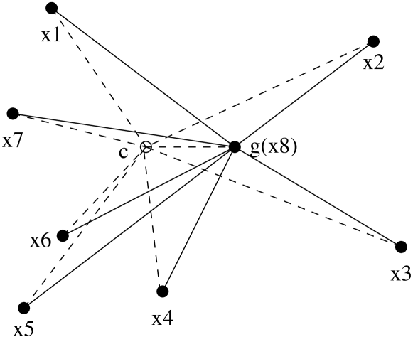
Figure 3: Edit Distances in Parse Space

A diagrammatic view of what we intend to accomplish is presented in Figure 3. The filled points are the parses given as input. The point marked $c$ is the true parse, hidden from us unless we are willing to explore the entire space. The dotted lines represent the minimum possible edit distance. Those lengths are the cost of editing the true parse into the observed parses. Point $x_{8}$ is also marked $g$ because it is the centroid chosen by minimizing the sum of pairwise distances (using the algorithm given). The cost we incur by using it is represented by the solid lines. We are claiming that the edit distance using $g$ is less than twice the edit distance using $c$.

$$n\sum_{i}d(\pi_{i},g) \leq \sum_{i}\sum_{j}d(\pi_{i},\pi_{j})$$

$$K \doteq \sum_{i}\sum_{j}d(\pi_{i},\pi_{j})$$

$$\sum_{i}d(\pi_{i},g) \leq \frac{K}{n}$$ (8)

The next observation of interest is that even the optimal choice for a centroid must obey the triangle inequality. The true parse, the best parse in parse space, is denoted here by $c$.

$$\sum_{i}\sum_{j}d(\pi_{i},\pi_{j}) \leq \sum_{i}\sum_{j}\left(d(\pi_{i},c)+d(c,\pi_{j})\right)$$

$$= 2(n-1)\sum_{i}d(\pi_{i},c)$$

$$\sum_{i}d(\pi_{i},c) \geq \frac{K}{2(n-1)}$$ (9)

Now we have bounded our hypothesis, $g$, from above with respect to $K$, and the optimal parse, $c$, from below with respect to $K$. This gives us a way to bound the extra cost we incur by using this suboptimal choice using simple substitution from Equations 8 and 9.

$$\frac{\sum_{i}d(\pi_{i},g)}{\sum_{i}d(\pi_{i},c)}\leq\frac{2(n-1)}{n}<2$$ (10)

In Equation 10 we see that the number of edits required to change our hypothesis, $g$, into each of the other parses is less than twice the number of edits required to change the optimal centroid hypothesis, $c$, (from the space of all parses) into the observed parses. We take this to be a reassuring bound on this approximation, as it was unlikely we could explore the space of parses to find $c$ in the first place.

The bound that we have just derived is interesting theoretically, but we cannot measure its behavior empirically because we are not able to find the optimal centroid hypothesis for comparison with the candidate that is picked. We did, however perform an experiment to address the effect of this heuristic. Consider picking the worst candidate for the centroid approximation instead of the best. The result for using that method is given under the entry bad distance in Table 7. Picking a centroid at random is the same as picking a parser at random, so that result would be approximately the same as the average individual parser accuracy. In short, we see that picking according to the heuristic with the provable bound gives significantly better results than these other (admittedly weak) techniques.

Technique	P	R	(P+R)/2	F	Exact
Best Individual	88.73	88.54	88.63	88.63	34.9
similarity	89.50	89.88	89.69	89.69	35.3
distance	90.24	89.58	89.91	89.91	38.0
bad distance	82.70	82.81	82.75	82.75	20.9
average performance	87.14	86.91	87.02	87.02	30.8

Table 7: Non-parametric Parser Switching

Combining with these algorithms produces the results in Table 7. The similarity switching parser is a better parser than any of the individual parsers and it gets higher recall than combining the parsers with constituent voting. However, the loss of precision makes the overall performance suffer. The distance switching parser is significantly better at precision and exact sentence accuracy than the similarity switching parser. The loss it incurs in recall is significant, but it is more than offset by the gain in precision, as we can see by the significantly different F-measure. We can see that the penalty the distance measure places on sentences with more constituents is appropriate in this case, as it correctly penalizes the parses that over-generate.

One of the main advantages of the parser switching framework is that the final predictions are as useful as the input because they maintain all the constraints that the input parses maintain. There are no crossing brackets, and as long as the switching algorithm is reasonably unbiased the trees are as dense as the input trees. If there are limits on the productions available for the parsers and the input parsers obey this limit, then we can guarantee our output will have the same guarantee. This can be important, for example, if we are dealing with a translation grammar that is specified as operations on productions in the grammar, or if we have partial database queries or other semantic information associated with the nodes in the parse tree. Maintaining an entire tree intact allows us to guarantee that we do not invalidate the translation or the database query in the process of producing a better hypothesis.

The secondary advantage we will see later is that it performs better at getting sentences exactly correct than the hybridization methods of constituent voting and naïve Bayes constituent combination.

10.3 Parse Tree Alignment

We have observed that parsing using a simple edit distance between parses proportional to the number of mismatched constituents gives us good results. There is no reason to believe that this particular choice of edit distance is the best one, though. In this section we explore other edit distances, and provide a general technique for editing complete parses using arbitrary (but constrained) costs of editing constituents.

The edit distance based on mismatched constituents is very coarse-grained. It allows no partially-matched constituents, which we might desire. Consider the sentence:

He mowed the grass down.

There are at least two acceptable parses for this sentence based on different interpretations of the word down. In Parse 10.3, the man is mowing down the grass, probably with a lawn mower, but perhaps with an automatic rifle. In Parse 10.3, the man is mowing something that is a cross between grass and soft fine feathers. If we keep only the matching constituents from those two parses, we get the structure in Parse 10.3. It gives no hint that the verb is transitive and there is very likely a noun phrase included inside the verb phrase. We have lost some information from these hypotheses that we would like to preserve.

S NP He VP mowed NP   the grass   down (3.1)

S NP He VP mowed NP   the grass down (3.2)

S NP He VP   mowed the grass down (3.3)

If a third parser produced Parse 10.3, we would feel very confident that $grass$ is part of a noun phrase inside the verb phrase, even if we had no other knowledge of English. Keeping only the matching constituents from any pair, or all of the parses (10.3, 10.3, and 10.3), we still arrive at Parse 10.3. This is precisely because the matched constituent edit distance does not differentiate in any way among the differences between these parses. The distance between any pair under this metric is exactly two edits: one constituent must be removed, and one inserted.

S NP He VP mowed      the NP   grass down (3.4)

The only way we should prefer Parse 10.3 (which we do), is if it is cheaper to edit it into both Parses 10.3 and 10.3 than it is to edit them into each other.

We have found a set of constituents that should have been edited in a way that yields an intuitive cost structure that does not match the reality of the distance measure we are using. It seems that it should be easy to work out a distance that is compatible with our intuition on a constituent-by-constituent basis. To this end we will describe a novel method for utilizing a given constituent-by-constituent editing cost function for computing an edit distance (and alignment) between complete parses.

Consider the relationship between alignment and editing. By alignment we mean a relation between the sets of constituents in two parses. In practical terms, an alignment describes a mapping between constituents in one parse and constituents in another parse, where any particular constituent needs not be mapped.

Each alignment corresponds to editing one set of constituents into another. Constituents that are not mapped (in the relation) are said to be insertions or deletions depending on which way the editing operation is being viewed. All of the rest of the nodes are substitutions, one (or many) for the other. In this way we can view the elements of the relation together with the constituents missing from the relation as editing operations. Several facts quickly become clear:

• For each alignment there is a unique editing cost. That is the sum of the cost of substituting the constituents in the relation together with the cost of inserting the constituents not involved in the relation.

• Depending on the editing cost function, there may be many alignments that produce the same editing cost between sets of constituents. We need only give an example to prove this. Consider the distance function we gave earlier, mismatched constituents. If we have two constituents on the left hand side that match a single constituent on the right hand side, it will be cheapest to align a pair of them, and the remainder remains unaligned. The choice we make in picking which constituent from the pair yields our proof.

• The minimal edit distance between sets of constituents can be proven by showing an alignment for the set whose cost is the edit distance. The alignment is a certificate for the edit distance.

• Verifying an alignment associated with an edit distance is a polynomial undertaking because verifying the alignment itself is polynomial (given that the edit cost function is polynomial). Unless there is some algebraic shortcut, verifying a minimal edit distance will require us to find an alignment. For this reason it is typically considered more prudent (and possible) to set out to find the minimal alignment first, instead of looking for shortcuts to computing a minimal edit distance.

Below we will give a polynomial algorithm for finding minimum-cost alignments with a few constraints on the edit cost function via a reduction to finding a minimum weight edge cover of a bipartite graph.

Both Oflazer [76] and Calder [20] have previously presented techniques for aligning linguistic trees. Oflazer’s technique first converts the tree representation into a list of paths from the root to the leaves of the tree. It then compares those path lists using standard dynamic programming approaches to computing edit distance. The motivation for his approach is computing approximate match between trees to facilitate database search. It is not clear that the induced alignment between the path lists represents simple edit operations on trees.

Calder’s technique for aligning trees is a bottom-up exact match strategy. A correspondence between the yields of two trees is made, and once grounded on that map between yields, the constituents can be compared by comparing their yields. This technique allows no partial constituent matches, and is well suited to producing alignments with the goal of comparing parses to a reference corpus.

Our work is significantly different from Calder’s in that we are not requiring aligned constituents to be strictly nested one inside the other. We are implicitly ignoring the global structure in picking aligning constituents, and we explore many distance measures between constituents. Furthermore, our algorithm is arrived at from a different set of constraints than Calder’s. The work is different from Oflazer’s tree-matching algorithm in that this work is not performing an approximate match. We are directly minimizing the metrics we show. Our representation is different from Oflazer’s, as well. We use a bag of constituents, and he uses a vertex list sequence.

10.3.1 Constraints and Formalities

We assume we are given a well-defined distance (edit cost) between constituents. By well-defined we mean:

• The edit distance be strictly positive, $d(X,Y)\geq 0$. Negative costs for edits are meaningless.

• The distance must be conservative, $d(X,X)=0$. There is no editing cost required to leave a constituent unedited.

• The distance must be symmetric, $d(X,Y)=d(Y,X)$. Editing is naturally a symmetric operation, as an insertion into on parse is equivalent to a deletion from the other. Also, substitutions should cost the same amount regardless of their directionality.

• The distance must handle insertions and deletions by recognizing the $NULL$ constituent, $d(X,NULL)$. The cost of deleting a constituent $X$ is $d(X,NULL)$. To preserve symmetry we must likewise constrain the cost of inserting a new constituent to $d(X,NULL)$.

• We do not want to constrain the distance to prevent constituents from moving large distances, or even outside of parenting constituents.

We will give the parse editing (alternatively alignment) process some liberty, especially in light of the constraints imposed by the edit distance criteria. Our requirements for the parse alignment are:

• Each left side constituent must map to zero, one, or more right side constituents. The mapping to zero constituents will be indicated by an alignment with $NULL$.

• We want to recover the cheapest alignment, corresponding to the cheapest sequence of constituent edits producing the right side parse from the left side parse.

• The edit distance associated with the alignment must be symmetric and obey the triangle inequality. This is so we can use it in conjunction with the distance-based parser switching algorithm and still enjoy the good performance bounds from Lemma 10.2.

10.3.2 Edge Covering Weighted Bipartite Graphs

Algorithm 3.4: Aligning Parses by Aligning Constituents

1. From the two parses, $\pi_{i}$ and $\pi_{j}$, for a sentence create the constituent sets $S_{i}$ and $S_{j}$ in the usual fashion.

2. Add the distinguished element, $NULL$, to each of the constituent sets.

3. Create a bipartite graph, $G=(V,E)$, with bipartition $(S_{i},S_{j})$ such that $E\subseteq(S_{i}\times S_{j})$.

4. Let each edge be weighted by the cost of editing between its endpoints into each other: $w(v_{1},v_{2})=d(v_{1},v_{2})$.

5. Convert to linear program. We want to find $a_{ij}$ to minimize

   $$\sum_{(v_{i},v_{j})\in E}a_{ij}w(v_{i},v_{j})$$ (11)

   subject to the constraints that the vertices must be covered by at least one incoming or outgoing edge:

   $$(\forall v_{i})\sum_{v_{j}\in S_{j}}a_{ij}\geq 1$$ (12)

   $$(\forall v_{j})\sum_{v_{i}\in S_{i}}a_{ij}\geq 1$$ (13)

6. Those edges for which the corresponding $a_{ij}=1$ are the ones included in the final alignment.

It is well known that solving these types of linear programs results in integer (binary in this case) weights on the edges [48]. In these cases we are solving what looks like an NP-complete integer programming problem using available polynomial algorithms for linear programming.

Recall that linear programming is a technique for maximizing or minimizing a linear function subject to a convex set of constraints. The simplex algorithm is a worst-case exponential time algorithm for solving linear programming instances, but the bad cases are rare. The simplicity of the implementation of the simplex algorithm makes it the algorithm of choice for most linear programming applications, even though there exist theoretically better (polynomial) algorithms for finding solutions. Furthermore, the bad cases for the simplex algorithm are rare. In our experiments, use of the simplex algorithm was not a bottleneck. It is much faster than the individual parsers we combined.

The alignment produced by the algorithm yields an edit distance between the two parses equal to the value of the resulting cover, $\sum\limits_{a_{ij}=1}a_{ij}d(v_{i},v_{j})$.

Figures 4 through 10 depict the steps of the algorithm as it would be run on an artificial but realistic example. The edge weights are omitted for aesthetic purposes.

Figure 4: Alignment – Two Parses As Bipartite Graph

Figure 5: Alignment – Adding Null Nodes

Figure 6: Alignment – Exact Matches Aligned

Figure 7: Alignment – Unaligned Nodes Are Fully Connected

Figure 8: Alignment – Remaining Forward Edges

Figure 9: Alignment – Remaining Reverse Edges

Figure 10: Alignment – Result of Linear Program

10.3.3 Constituent Edit Distances

To explore the utility of the alignment algorithm, we require a test bed of constituent alignment distances. We experimented with many different distances, and creating or choosing one remains an art. We may have implicitly over-fit our model to the development test data through our experimentation. This is one of the main shortcomings of non-parametric methods, and it is very hard to avoid if one wants to do any exploration of non-parametric methods in an empirical research setting. The results on the separate test set are presented in section 12, and that evaluation provides a sanity check on the methods.

Here we will list a sampling of the distances we used, together with a brief description of each one. There are some notational issues to discuss first, though. If $X$ is a constituent, then we denote its label by $X_{l}$. Its left index is $X_{i}$ and its right index is $X_{j}$. If the constituent $X$ matches constituent $Y$ in all three of these features, we say $X=Y$. Individual predicates are conjunctively joined with “,” and disjunctively joined with “or”.

Finally, we must comment on our use of $\infty$ in the distance measures. Linear programs and linear programming packages typically require finite, real-valued weights. In order to accommodate this in a practical manner, we replaced the $\infty$ value in these distances with a number larger than the weight of any possible alignment excluding an $\infty$. We could bound the value by simply summing the weights on all the finite-weighted edges and doubling it. That value substituted for $\infty$ was large enough that we would notice them as spurious output when the program was run. As expected, no “infinite”-valued edge was ever chosen as an edge for an alignment.

$$d_{Kronecker}(X,Y)=\left\{\begin{array}[]{rl}0&X=Y\\ 1&X\neq Y\mbox{, }X=NULL\mbox{ or }Y=NULL\\ \infty&X\neq Y\mbox{, }X\neq NULL\mbox{, }Y\neq NULL\end{array}\right.$$ (14)

The first distance, named Kronecker after the Kronecker delta function, is given in Equation 14. The value for this alignment is the number of mismatched constituents, as they will each be aligned to $NULL$ with a cost of 1.

$$d_{piecewise}(X,Y)=\left\{\begin{array}[]{rl}0&X=Y\\ 2&X\neq Y\mbox{, }X=NULL\mbox{ or }Y=NULL\\ 3&\mbox{only one of}\left\{\begin{array}[]{l}X_{i}\neq Y_{i}\\ X_{j}\neq Y_{j}\\ X_{l}\neq Y_{l}\end{array}\right.\\ \infty&\mbox{otherwise}\end{array}\right.$$ (15)

In Equation 15 we have a distance that is similar to the Kronecker distance, except that it allows a pair of constituents to be aligned to each other if they differ in exactly one feature: label, left index, or right index. The cost of such a matching is 3, versus a cost of 4 to align each of the constituents to the corresponding $NULL$ (a cost of 2 for each of the mismatched pair).

$$d_{looselabel}(X,Y)=\left\{\begin{array}[]{rl}0&X=Y\\ 2&X\neq Y\mbox{, }X=NULL\mbox{ or }Y=NULL\\ 3&X_{i}=Y_{i}\mbox{, }X_{j}=Y_{j}\mbox{, }X_{l}\neq Y_{l}\\ \infty&X_{i}\neq Y_{i}\mbox{ or }X_{j}\neq Y_{j}\end{array}\right.$$ (16)

The looselabel distance given in Equation 16 is similar to the piecewise distance, except only the label on the constituent is allowed to mismatch.

$$d_{linear}(X,Y)=\left\{\begin{array}[]{rl}0&X=Y\\ X_{j}-X_{i}&Y=NULL\\ Y_{j}-Y_{i}&X=NULL\\ \infty&X_{l}\neq Y_{l}\\ \infty&X_{i}\neq Y_{i},X_{j}\neq Y_{j}\\ |X_{j}-Y_{j}|+|X_{i}-Y_{i}|&\mbox{otherwise}\end{array}\right.$$ (17)

The linear edit distance given in Equation 17 is an attempt to penalize editing constituents that have wildly different spans into each other. It does so by assigning a cost to editing constituents proportional to the difference in spans between the constituents. It also requires that the labels on the constituents match, as well as at least one edge. This is not the first distance we tried that introduced linear penalties for editing constituents, but it was one of the better ones.

$$d_{stringent}(X,Y)=\left\{\begin{array}[]{rl}0&X=Y\\ 2&Y=NULL\mbox{ or }X=NULL\\ \infty&X_{i}\neq Y_{i}\mbox{, }X_{j}\neq Y_{j}\\ \infty&X_{l}\neq Y_{l}\mbox{, }(X_{i}\neq Y_{i}\mbox{ or }X_{j}\neq Y_{j})\\ 3&X_{l}\neq Y_{l},X_{i}=Y_{i},X_{j}=Y_{j}\\ 3(|X_{j}-Y_{j}|+|X_{i}-Y_{i}|)&\mbox{otherwise}\end{array}\right.$$ (18)

The stringent distance allows constituent labels to mismatch if the spans are the same, and it allows one edge of the span to mismatch if the label and the other edge of the span is the same. Still, it does not allow the span to mismatch by more than one token.

Distance	P	R	(P+R)/2	F	Exact
linear	90.04	89.39	89.71	89.71	38.0
piecewise	90.17	89.55	89.86	89.86	38.0
Kronecker	90.22	89.55	89.88	89.88	37.9
loose label	90.26	89.63	89.95	89.95	38.3
stringent	90.27	89.63	89.95	89.95	38.3
Best Individual	88.73	88.54	88.63	88.63	34.9

Table 8: Parser Switching Using Centroid Approximation

In Table 8 we see the result of performing distance-based parser switching using the alignment cost produced us the various constituent edit distances. The leftmost column indicates the constituent edit distance that was used in conjunction with the alignment and distance algorithms. The other columns are the same as in the other performance tables. The difference between the piecewise and Kronecker models is not significant, and neither is the difference between the loose label and stringent systems.

It appears that the loose label distance is the best one to use for aligning Treebank parses. This could be because there are constituent labels in the Treebank that behave similarly enough that interchanging them does not make a big difference on resolving syntactic ambiguity. Another reason could be that the weaker parsers might be good at finding the spans for constituents but not as good at labelling them.

The performance difference between the Kronecker system and the previously discussed distance-based parser switching algorithm using mismatched constituents is a result of the two programs breaking ties in a different (arbitrary) way. The two algorithms are equivalent in analysis otherwise. We can see from this how little the arbitrary tie-breaking affects performance. Ties were broken in the same manner for all of the systems in Table 8.

10.3.4 The Consensus Parse

This method for approximating centroids in the parse space can also be used as a first step for building a new kind of consensus parse, similar to constituent voting.

Given these alignments between pairs of parses and a threshold $t$, we can build an ad hoc hybrid parse in the following way:

Algorithm 3.5: Consensus Parse from Pairwise Alignments

Input: Bipartite alignment graphs and cost threshold $t$ for deciding when to stop hypothesizing constituents.

1. Initialize $C$ to the empty set and $G$ as the obvious union of the bipartite alignment graphs.

2. Merge all $NULL$ nodes in $G$.

3. For each constituent $c$ in each parse, compute the cost $f(c)$ to edit that constituent into each of its neighbors $N(c)$ given by the alignments.

   $$f(c)=\sum_{c^{\prime}\in N(c)}d(c,c^{\prime})$$ (19)

4. Let $c^{*}=\mathop{\rm argmin}\limits_{c\in V(G),c\neq NULL}f(c)$

5. If $(f(c^{*})>t)$ then output the current hybrid, $C$ and quit.

6. $C\leftarrow C\cup\{c^{*}\}$.

7. Remove $c^{*}$ and all $c^{\prime}\in N(c)$ from $G$.

8. If the graphs are empty (aside from $NULL$), output $C$ and quit.

This is an ad hoc greedy algorithm, attempting to maximize the confidence on the constituents that are being put into the hybrid. Typically $t$ is chosen to match the constituent editing function and in the same manner, not by estimating it on data.

Distance	P	R	(P+R)/2	F
linear	87.89	89.27	88.58	88.58
piecewise	92.24	88.83	90.54	90.50
stringent	92.11	89.13	90.62	90.60
loose label	92.10	89.15	90.63	90.60
Kronecker	92.09	89.18	90.64	90.61
Best Individual	88.73	88.54	88.63	88.63

Table 9: Parser Switching Using Consensus Approximation

10.3.5 Limitations

We build the consensus in this ad hoc, greedy fashion because we must work with pairwise alignments. Multiple alignments of this sort are intractable as we add parsers, and it is not clear what goodness measure we would want to maximize in producing a multiple alignment in the first place. In short, edge covering $k$-partite graphs is exponential in $k$. This algorithm is a greedy approximation to it.

11 Adding Parameters

Non-parametric methods help us develop initial results and get a sense for the feasibility of our method. In this section we develop parametric versions of combining by constituent voting and parser switching. We use few parameters in this process because we have very little training data. Estimating too many parameters will undoubtedly yield a model with estimates based on insufficient statistics.

11.1 Independent Constituents

As in the non-parametric case, each member hands the combiner a set of tuples of the form $(s,e,l)$ for each sentence, where $s$ is the start index for the constituent, $e$ is the ending index, and $l$ is the label.

We then formulate the combination of voters as a binary classification problem. First we make the constituency independence assumption: assume each constituent is independently selectable. This is inconsistent with the notion of a parse tree, but it can still produce a useful structure.

For each constituent $c$ we are interested in $P(\pi(c)|M_{1}\ldots M_{k})$ where $M_{i}$ is the random variable which takes a value from $\{true,false\}$ depending on whether parser $i$ contains that constituent in its final parse.

We can use a naïve Bayes model [35] to produce an estimate of this probability. Naïve Bayes makes the assumption that all of the random variables we condition on are independent. This assumption exactly matches the assumption we are making in endeavoring to combine these parsers in the first place. In this way the naïve Bayes modeling technique is well matched to our problem.

In more detail we first uses Bayes’s law to make the transformation:

$$P(\pi(c)|M_{1}\ldots M_{k}) = \frac{P(M_{1}\ldots M_{k}|\pi(c))P(\pi(c))}{P(M_{1}\ldots M_{k})}$$ (20)

Then we assume the $M_{i}$ variables are pairwise independent.

$$P(\pi(c))\frac{P(M_{1}\ldots M_{k}|\pi(c))}{P(M_{1}\ldots M_{k})} = P(\pi(c))\prod_{i=1}^{k}{\frac{P(M_{i}|\pi(c))}{P(M_{i})}}$$ (21)

We can throw away the denominator because we are actually only interested in the value of $\pi(c)$ that is larger. We can then transform the expression into terms we can collect from a corpus.

$$P(\pi(c))\prod_{i=1}^{k}{\frac{P(M_{i}|\pi(c))}{P(M_{i})}} = P(\pi(c))\prod_{i=1}^{k}{P(M_{i}|\pi(c))}$$ (22)

$$P(\pi(c)=true)\prod_{i=1}^{k}{P(M_{i}|\pi(c)=true)}=$$ (23)

$$\frac{C(\pi(c)=true)}{\sum_{X}{C(\pi(c)=X)}}\prod_{i=1}^{k}{\frac{C(M_{i},\pi(c)=true)}{C(\pi(c)=true)}}$$

The $C(\bullet)$ family of functions return the count instances of co-occurrences of their arguments in a training set.

We use Laplacian (sometimes Lidstone’s) smoothing while estimating to avoid assigning zero probability to novel events [61, 65]. Laplacian smoothing, sometimes known as “add-one” smoothing, is equivalent to adding one to the number of times each possible event was seen in the corpus before estimating probabilities. Lidstone’s smoothing is similar, except an unspecified parameter, $\lambda$ is added to the number of times each possible event was seen. Both smoothing schemes are linear combinations of the observed frequencies with the uniform distribution.

This is the simplest form of a naïve Bayes classifier for this problem. It uses one parameter per parser. On our training set it performs identically to the second row of Table 6. This is not surprising since we are using only three parsers and they differ very little in accuracy. The robustness of this model when adding a poor parser is described in Section 12.

11.1.1 Context

There are a number of candidate contexts that may indicate how we should distribute our trust across the ensemble members:

• Constituent Label ($l$)

• Constituent length ($e-s$)

• Parent label (ancestor label)

• Sentence length

Polling pattern (i.e. for candidate constituent $x$, $\pi_{1}(x)=1\wedge\pi_{2}(x)=0\wedge\pi_{3}(x)=1$) is not a reasonable candidate for a context. There are too many polling patterns to choose from (the set grows exponentially in the ensemble size). The parameter space is simply too large to yield any reliable probability estimates on our small datasets.

In the following formulation, $\pi(c)$ is the binary random variable we are estimating. Its value indicates whether we feel this constituent should be in the parse. $T$ is the random variable indicating the label (e.g. NP, VP) on the constituent. $M_{i}$ is the binary prediction parser $i$ provides for the particular labelled constituent in question. Alternatively, for some $i$, $M_{i}$ can describe the value of contextual features around the constituent in question. In fact, one can view the votes of the member parsers as merely more features to throw into the classifier. We call this model the Coprediction Model. It requires many parameters, specifically $O(kn)$ where $k$ is the number of values the copredicting feature can take on and $n$ is the number of parameters in a model without context.

$$P(\pi(c),T=t|M_{1}\ldots M_{k}) = \frac{P(M_{1}\ldots M_{k}|\pi(c),T)P(\pi(c),T)}{P(M_{1}\ldots M_{k})}$$ (24)

$$= P(\pi(c),T)P(M_{1}\ldots M_{k}|\pi(c),T)$$ (25)

$$= P(\pi(c),T)\prod_{i=1}^{k}{P(M_{i}|\pi(c),T)}$$ (26)

$$P(\pi(c)|T,M_{1}\ldots M_{k}) = \sum_{t}P(\pi(c),t)P(M_{1}\ldots M_{k}|\pi(c),t)$$ (27)

This derivation is exactly the same as in Equation 21 except that we are predicting both membership in the parse and the context of the parse. Since we are sure of the context of the parse, the result we use is $P(\pi(c),T=t)$ where $t$ is the particular observed context. The probabilities are estimated similarly to those in Equation 23.

Another way to add context is shown below. We call this the Independent Context Model. Here the context serves only to change the threshold at which we use our estimate of $P(\pi(c)|M_{1}\ldots M_{k})$. We adjust the threshold by $P(T|\pi(c))$ to account for the particular context we observe. This process can easily be repeated by inserting an adjustment factor for each of the contexts desired. This formulation uses as few parameters as possible among formulations including contexts. It needs only $O(k+n)$ where $k$ and $n$ are as we mentioned before. Since so few parameters are needed, it is much easier to gather sufficient statistics for each of them. It is crucial that the contexts be independent in this case, as well as independent of the predictors, as that is the assumption we use to move from Equation 29 to Equation 30.

$$P(\pi(c)|T,M_{1}\ldots M_{k}) = \frac{P(M_{1}\ldots M_{k}|\pi(c),T)P(\pi(c))}{P(T,M_{1}\ldots M_{k})}$$ (28)

$$= P(\pi(c))P(T,M_{1}\ldots M_{k}|\pi(c))$$ (29)

$$= P(\pi(c))P(T|\pi(c))\prod_{i=1}^{k}{P(M_{i}|\pi(c),T)}$$ (30)

In the Coprediction Model, we are predicting the label on the constituent and its membership in the hypothesis parse simultaneously given the predictions of the parsers. In the Independent Context Model we first predict the label given the predictions of the parsers, and then membership in the hypothesis parse based on the label and the predictions of the parsers.

These models are each somewhat arbitrary ways to introduce context without requiring a tabular estimation of the entire joint distribution $P(\pi(c),M_{1}\ldots M_{k})$. The reason we avoid it is that we expect the size of the ensemble to eventually grow to include many parsers. As $k$ gets large, filling the table to estimate that distribution directly from relative frequencies requires a large corpus that could potentially be better used to train the member parsers.

We tested each of these models of context on our parser outputs using the contexts described above. The results can be seen in Table 10. The model types are indep or copredict to describe whether the particular model was using the coprediction or independent context techniques. Among the contexts, tag represents the tag on the constituent (e.g. NP, VP), parenttag represents similarly the tag on the parent constituent, clength is a continuous feature representing the span of the constituent, and slength is the length of the sentence. The singular appearance of tag&parenttag represents a feature whose values are pairs consisting of the tag of the constituent and the tag of the parent of the constituent.

Fewer and smaller contexts are used with the coprediction model because of the way it blows up the parameter space. These results are from the training set, the same set used for estimating the probabilities. None of the context added to the model gave large improvements to the F-measure.

Model	Context	P	R	(P+R)/2	F
indep	tag,clength,parenttag	91.81	89.10	90.46	90.43
copredict	tag	91.26	89.71	90.49	90.48
indep	clength	91.63	89.43	90.53	90.52
indep	tag&parenttag	91.96	89.17	90.56	90.54
indep	tag	92.05	89.22	90.63	90.61
indep	slength	92.06	89.20	90.63	90.61
copredict	clength	92.14	89.15	90.64	90.62
copredict	slength	91.95	89.44	90.69	90.68
Best Individual		88.73	88.54	88.63	88.63
Naïve Bayes		92.09	89.18	90.64	90.61

Table 10: Results of Bayes with Context (Training Set)

11.1.2 Negative Results

The results in Table 10 are discouraging. None of the contexts added much to the predictive power of our models. Furthermore, the gain seen in the last row of that table versus combining by non-parametric democratic voting or by context-less naïve Bayes is not enough to show that the training set precision and recall of the hypotheses are significantly different in their predictions on the training set at a 90% confidence level. In short, nothing helped. The estimation error induced by using these models and adding parameters overshadowed any reduction we achieved by utilizing more descriptive models.

We cannot prove that there is not some set of contexts that will give us a gain in accuracy. However, we can analyze our data using these particular contexts to get a feel for why context does not provide a gain. In particular, we are interested in instances where it is desirable to trust one parser more than the consensus of the other two parsers. If there is no context in which a single parser performs better than the other two, then there is no way we can use context information to perform better than majority vote or simple naïve Bayes.

A statistic we are interested in is the precision of a parser on those samples for which it disagrees with the majority opinion. In our scenario this can only happen when the other two parsers agree and the parser in question disagrees with their hypothesis. The formula for the precision is given in Equation 31 where $\mathop{\rm majority}$ is the operator that produces a set consisting of elements appearing in a majority of the given sets, and $S_{P_{i}}$ is the set of constituents produced by Parser $i$. We call the measure isolated precision because it is the precision the parser can achieve on constituents that only it believes should be in the parse. When the isolated precision is less than 50%, adding the constituents in question to the set will result in adding more errors than correct predictions. When it is greater than 50%, adding those predictions will result in a gain over the majority predictor. We can get some idea of whether partitioning the prediction space using a particular context will be helpful by looking for places in that partitioning where the isolated precision is greater than 50%.

$$P_{isolated}(P_{i}) = \frac{|(S_{P_{i}}-\mathop{\rm majority}\limits_{j\not=i}S_{P_{i}})\cap S_{true}|}{|S_{P_{i}}-\mathop{\rm majority}\limits_{j\not=i}S_{P_{i}}|}$$ (31)

Constituent	Parser1		Parser2		Parser3
Label	count	P	count	P	count	P
ADJP	132	28.78	215	21.86	173	34.10
ADVP	150	25.33	129	21.70	102	31.37
CONJP	2	50.00	8	37.50	3	0.00
FRAG	51	3.92	29	27.58	11	9.09
INTJ	3	66.66	1	100.00	2	50.00
LST	0	NA	0	NA	0	NA
NAC	0	NA	13	53.84	7	14.28
NP	1489	21.08	1550	18.38	1178	27.33
NX	7	85.71	9	22.22	3	0.00
PP	732	23.63	643	20.06	503	27.83
PRN	20	55.00	33	54.54	38	15.78
PRT	12	16.66	20	40.00	16	37.50
QP	21	38.09	34	44.11	76	14.47
RRC	1	0.00	1	0.00	2	0.00
S	757	13.73	482	23.65	434	38.94
SBAR	331	11.78	196	23.97	178	34.83
SBARQ	0	NA	6	16.66	3	0.00
SINV	3	66.66	11	81.81	13	30.76
SQ	2	0	11	18.18	3	33.33
UCP	6	16.66	12	8.33	8	12.50
VP	868	13.36	630	24.12	477	35.42
WHADJP	0	NA	0	NA	1	0.00
WHADVP	2	100.00	5	40.00	1	100.00
WHNP	33	33.33	8	25.00	17	58.82
WHPP	0	NA	0	NA	2	100.00
X	0	NA	2	100.00	1	0.00

Table 11: Isolated Constituent Precision By Context

Parent	Parser1		Parser2		Parser3
Label	count	P	count	P	count	P
ADJP	46	30.43	87	20.68	58	24.13
ADVP	21	19.04	31	22.58	26	34.61
FRAG	37	21.62	10	0.00	9	33.33
NAC	0	NA	3	66.66	2	100.00
NP	1081	22.57	1320	19.01	1034	25.82
NULL	194	0	0	NA	0	NA
NX	4	100.00	0	NA	0	NA
PP	445	26.06	447	21.47	360	27.77
PRN	27	59.25	22	40.90	28	25.00
RRC	1	0.00	1	0.00	1	0.00
S	1111	10.53	672	22.47	543	33.70
SBAR	240	19.58	184	24.45	177	35.02
SBARQ	0	NA	8	50.00	4	25.00
SINV	15	60.00	33	27.27	16	31.25
SQ	6	33.33	11	27.27	9	33.33
TOP	8	100.00	59	30.50	24	37.50
UCP	4	25.00	9	44.44	2	100.00
VP	1378	20.10	1146	22.94	952	34.24
WHADJP	1	100.00	0	NA	0	NA
WHADVP	0	NA	3	66.66	0	NA
WHNP	1	0.00	2	50.00	7	71.42
WHPP	0	NA	0	NA	0	NA
X	2	100.00	0	NA	0	NA

Table 12: Isolated Constituent Precision by Parent Label

Tables 11 and 12 give values for $P_{isolated}(P_{i})$ under restriction to constituent label and parent’s constituent label contexts respectively. Notice that in most of the situations in which the precisions are greater than 50% the number of times those contexts appear is insignificant. In the training set from which these numbers were calculated a 0.1 percent improvement in precision requires approximately 40 more correct predictions (or about 40 fewer incorrect predictions).

Figure 11: Isolated Constituent Parser Precision and Sentence Length

Figure 12: Isolated Constituent Parser Precision and Span Length

The graphs in Figures 11 and 12 show how the same value varies by sentence length and constituent length respectively. We see the same effect in these graphs. When the graph of isolated precision is over 50%, the number of occurrences of the particular context is so small that the possible gain is small and often insignificant.

In Tables 13 and 14 we break down the (standard) precision that each parser is able to attain by the constituent label and the label on the parent of the constituent. This gives us an idea of how the parsers perform in isolation and how little they differ in assorting their accuracy across the constituent types.

From Table 13 we can calculate the precision and recall we can achieve by assembling a parser that decides to trust the most precise parser for each constituent. For example, we would trust Parser3 for constituents with label NP because it has the highest precision for that label. If we built this parser we would get a precision of 88.97% and a recall of 88.07%. This yields an F-measure of 88.52%, substantially worse than the best individual parser. The F-measure is worse because precision goes up but recall would decrease in this case when compared to the best individual parser.

Our goal is to maximize F-measure but we picked the parser with the highest precision for each of the partitions induced by the constituent label context. This is not because choosing in this manner maximizes F-measure. F-measure is a global measure, and as such is very hard to maximize [45]. This is because an imbalance favoring precision for one partition and an imbalance favoring recall for another partition can combine to yield a higher F-measure than when the partitions are individually set to optimize F-measure.

Constituent	Parser1		Parser2		Parser3
Label	count	P	count	P	count	P
ADJP	688	75.58	832	68.75	810	73.95
ADVP	1227	82.23	1182	82.74	1195	85.02
CONJP	19	73.68	25	64.00	15	60.00
FRAG	65	13.84	43	32.55	14	14.28
INTJ	8	87.50	6	83.33	9	77.77
LST	4	100.00	3	100.00	2	100.00
NAC	5	100.00	24	75.00	19	68.42
NP	18747	88.92	18884	88.39	18718	90.25
NX	10	90.00	12	41.66	3	0.00
PP	5620	82.36	5544	81.78	5530	84.61
PRN	102	85.29	114	81.57	116	68.96
PRT	142	77.46	177	76.27	170	77.05
QP	472	88.77	503	85.88	539	78.47
RRC	1	0.00	2	0.00	3	0.00
S	5753	83.45	5584	88.07	5671	89.70
SBAR	1776	78.15	1703	85.49	1742	87.25
SBARQ	4	75.00	10	40.00	7	57.14
SINV	28	78.57	141	92.19	149	88.59
SQ	10	80.00	22	59.09	15	86.66
UCP	11	45.45	22	40.90	17	52.94
VP	8811	85.81	8733	89.12	8758	90.64
WHADJP	3	66.66	1	0.00	4	50.00
WHADVP	122	96.72	130	93.07	124	95.96
WHNP	438	93.60	293	96.92	423	96.69
WHPP	21	100.00	17	100.00	25	100.00
X	1	100.00	4	100.00	3	66.66

Table 13: Constituent Precision By Context

Parent	Parser1		Parser2		Parser3
Label	count	P	count	P	count	P
ADJP	362	80.38	410	72.43	390	77.17
ADVP	216	83.33	221	81.90	230	83.47
FRAG	72	55.55	49	71.42	48	85.41
NAC	2	100.00	6	83.33	6	100.00
NP	10670	85.41	10831	83.63	10661	85.90
NULL	194	0.00	0	NA	0	NA
NX	8	100.00	4	100.00	3	100.00
PP	5621	88.82	5667	87.87	5636	89.51
PRN	149	81.87	151	74.17	154	70.12
RRC	1	0.00	1	0.00	1	0.00
S	11232	87.38	10975	91.37	11019	92.59
SBAR	2315	86.86	2198	88.85	2369	90.20
SBARQ	10	100.00	21	80.95	17	82.35
SINV	339	94.98	442	92.30	445	95.05
SQ	30	80.00	36	69.44	34	76.47
TOP	2294	97.25	2431	96.25	2409	97.50
UCP	29	89.65	36	86.11	27	100.00
VP	10501	81.92	10489	83.14	10583	85.39
WHADJP	1	100.00	0	NA	0	NA
WHADVP	0	NA	3	66.66	0	NA
WHNP	14	78.57	12	91.66	20	80.00
WHPP	24	100.00	25	100.00	25	100.00
X	4	100.00	3	100.00	4	100.00

Table 14: Constituent Precision by Parent Label

We should not be surprised that the contexts we investigate make little difference in our decision-making capability for combining these parsers. The parsers were all trained with these contexts (and more) in mind. Their creators have done a good job of taking advantage of the tendencies of certain structures to be found only in certain contexts.

11.1.3 Experiment: Adding a base noun phrase chunker

In order to again further test the efficacy of our context-dependent combination techniques, we added the Ramshaw and Marcus base noun phrase chunker [82] to the ensemble. The chunker attempts to predict which phrases appear as non-recursive noun phrases in a parse, the noun phrases that are lowest in the tree. It is designed for applications that do not require full parsing, and generally runs much faster than a full-blown parser. Ramshaw and Marcus used transformation-based learning to induce a set of transformation rules that can be quickly run over a large corpus to produce base NP brackets.

The expectation for adding the chunker to the ensemble was that the Bayes technique would learn to trust the chunker, or at least utilize the chunker’s decisions when dealing with NP tags.

Model	Context	P	R	(P+R)/2	F
indep	tag	91.62	89.44	90.53	90.52
copredict	tag	91.44	89.14	90.29	90.28
Best Individual		88.73	88.54	88.63	88.63
Naïve Bayes (3)		92.09	89.18	90.64	90.61
Naïve Bayes (4)		91.60	89.57	90.59	90.57

Table 15: Results of Including a Noun Phrase Chunker

In Table 15 we can see the result of using the independent constituents and coprediction models for combining the four systems. Both of these results are worse than the naïve Bayes model for the three parsers, as well as the naïve Bayes result when the chunker is added to the group. Also, both of these models predict with significantly lower precision than the naïve Bayes(3) model.

Model	P	R	(P+R)/2	F
Parser1	88.92	89.93	89.43	89.42
Parser2	88.39	90.05	89.22	89.21
Parser3	90.25	91.14	90.69	90.69
Majority(1-3)	93.30	92.17	92.73	92.73
NP chunker	93.59	68.87	81.23	79.34

Table 16: Parser Performance on Noun Phrases

Further study enables us to decide why we gained nothing from introducing such an intuitively appealing source of noun phrase annotations. In Table 16 we show the performance of the parsers and chunker on only those constituents that are labelled with NP. While the precision for the chunker is significantly higher than the majority vote of the three parsers, note that the recall for the chunker is much lower than the other systems. This happens because the chunker is predicting only non-recursive noun phrases. All noun phrases that contain a nested noun phrase are by definition not targets for the chunker to predict. That is why the combined system takes a performance hit when the chunker is added: when the chunker says a constituent should be a noun phrase it is a little more accurate than the majority vote, but when it says the constituent is not a noun phrase it is wrong on all of the non-base noun phrases.

To summarize the claims, we estimated the portion of the noun phrase constituent inclusion decisions that were correctly predicted by the chunker, and on which the majority of the three parsers disagreed. This value was only 48%, indicating that the chunker was performing worse than chance on predictions it was asked to make about constituents that it had a chance to help predict. This is probably not a coincidence. The chunker was only designed to predict the non-recursive noun phrases. Incorporating it into the combined model would require a specialized model that included a notion of “base-ness” of a noun phrase. While it could prove useful to pursue combination techniques in which such a feature can easily be specified, none of our models can take it directly into account.

11.2 Pruning into Trees

The parametric models we have developed so far have not enforced a tree constraint. There is nothing stopping these independently-predicted constituents from inducing crossing structures in the parse tree. In this case, pruning of the crossing constituents could be explored. Our negative results from this section did not suggest there would be any value in pursuing this line of research at the present time, though.

However, when we are using the simplest naïve Bayes configuration with no context, requiring estimated constituent probabilities strictly larger than 0.5 to include them in the parse, the result from Lemma 3.1 enables us to say that no crossing brackets will appear in the final hypothesis.

11.3 Parser Switching

Just as in Section 10.2, we can try to beat the Parser Switch Oracle using our models. As shown above, context gives us very little if any gain, so we will not incorporate it into our switching model. It could be the case that small gains in the naïve Bayes probability model can make larger gains in the switching algorithm, but that is not the purpose of this investigation. We first reformulate the problem as shown below. We are interested choosing the parse among the input parses that maximizes the probability of correctness for each of its constituents (and predictions on missing constituents). We treat those predictions as independent.

$$\mathop{\rm argmax}\limits_{\pi_{i}}P(\pi_{i}|M_{1}\ldots M_{k}) = \mathop{\rm argmax}\limits_{\pi_{i}}\prod_{c}{P(\pi_{i}(c)|M_{1}\ldots M_{k})}$$

$$= \mathop{\rm argmax}\limits_{\pi_{i}}\prod_{c}\frac{P(M_{1}\ldots M_{k}|\pi_{i}(c))P(\pi_{i}(c))}{P(M_{1}\ldots M_{k})}$$

$$= \mathop{\rm argmax}\limits_{\pi_{i}}\prod_{c}{P(\pi_{i}(c))\prod_{j=1}^{k}{\frac{P(M_{j}|\pi_{i}(c))}{P(M_{j})}}}$$

$$= \mathop{\rm argmax}\limits_{\pi_{i}}\prod_{c}{P(\pi_{i}(c))\prod_{j=1}^{k}{P(M_{j}|\pi_{i}(c))}}$$

P	R	(P+R)/2	F	Exact
90.13	89.65	89.89	89.89	38.4

Table 17: Naïve Bayes Parser Switching

The results (as shown in Table 17) are better than those achieved in the unsupervised, non-parametric parser switching experiment (from Table 7). Intuitively, this is because we have more faith in the predictions of the better parsers. The candidate parse that agrees more with the better parsers is preferred to those that agree more with the parsers that perform worse.

12 Final Evaluation

After developing all of our models we evaluated them on the 1700 sentences in the test corpus. This section gives a full account of those results.

12.1 Test Set

We have made some performance claims on our training data. The claims are summarized below and in Table 18.

1. A significant precision and recall boost can be attained using simple non-parametric democratic voting on constituents.

2. A significant precision and recall boost can be attained using non-parametric parser switching. This is useful when we want to preserve constraints on the productions in the parses.

3. A significant precision and recall boost can be attained using parametric parser switching, and the gain is larger than the non-parametric version.

4. Parser switching by approximating the centroid using parse edit distance suggests we can more precisely pick parses than by using Bayes parser switching. This is odd because this is an unsupervised method that surpasses the comparable supervised method. The difference in F-measure is merely suggestive, though.

Reference / System	P	R	(P+R)/2	F	Exact
Average Individual Parser	87.14	86.91	87.02	87.02	30.8
Best Individual Parser	88.73	88.54	88.63	88.63	35.0
Parser Switch Oracle	93.12	92.84	92.98	92.98	46.8
Maximum Precision Oracle	100.00	95.41	97.70	97.65	64.5
Similarity Switching	89.50	89.88	89.69	89.69	35.3
Distance Switching	90.24	89.58	89.91	89.91	38.0
Alignment Switching	90.26	89.63	89.95	89.95	38.3
Bayes Switching	90.13	89.65	89.89	89.89	38.4
Constituent Voting	92.09	89.18	90.64	90.61	37.0
Alignment and Consensus	92.10	89.15	90.63	90.60	37.0
Naïve Bayes	92.09	89.18	90.64	90.61	37.0

Table 18: Summary of Training Set Performance

In this section we evaluate the models that produced those claims on the 1700 sentences in the test set.

Reference / System	P	R	(P+R)/2	F	Exact
Average Individual Parser	87.61	87.83	87.72	87.72	31.6
Best Individual Parser	89.61	89.73	89.67	89.67	35.4
Parser Switch Oracle	93.78	93.87	93.82	93.82	48.3
Maximum Precision Oracle	100.00	95.91	97.95	97.91	65.6
Similarity Switching	90.04	90.81	90.43	90.43	36.6
Distance Switching	90.72	90.47	90.60	90.60	38.4
Alignment Switching	90.70	90.47	90.59	90.59	38.4
Bayes Switching	90.78	90.70	90.74	90.74	38.8
Constituent Voting	92.42	90.10	91.26	91.25	37.9
Alignment and Consensus	92.43	90.08	91.26	91.24	37.9
Naïve Bayes	92.42	90.10	91.26	91.25	37.9

Table 19: Summary of Test Set Performance

Table 19 shows the results. All of the parsers performed as well on this set as they did on their original test set. The best parser performed significantly better on this than on the original test set. One possible explanation for this is that this set contains many sentences that are systematically easier to parse. This is likely because these parses are not randomly partitioned. They were partitioned based on the order in which they were published. If, for example, the complexity of the news varies (and consequently contains simpler sentences) with respect to time, then we would expect to observe this behavior. Verifying this hypothesis is beyond the scope of this thesis, however.

We can push aside the question of baseline performance differences between the different testing corpus sections (22 and 23) because we are more interested in the improvement we can make via combination than the raw accuracy numbers. In some sense, if this dataset (section 22) is easier to parse, it should be harder to get a gain from combining parsers.

The combining techniques all perform substantially better on this set, probably because the developers (and reviewers of their published works) never investigated it. That is, the combining techniques reduce the error rate more on this set than on the previous set. There was no bias or incentive for performing well on this set, and implicitly training on the test set (either individually or through peer review) was not investigated. Implicit training on the test set tends to make the systems similar, because there exists a strong competitive drive to tune the systems to do at least as well as the other system on whatever metrics are used, rather than to simply perform well at modeling the phenomena in the corpora.

The big surprise from this set is that the Alignment Switching method (that rivaled Bayes Switching on the training set) performed very poorly on this set. This is probably due to excessive experimentation. We investigated many edit distance functions in building the algorithm and may have implicitly over-fit the training set by making our choice. This is a well-known shortcoming of the winner-takes-all approach to choosing between multiple algorithms during training [75]. The best algorithm for the training data is not the best algorithm for the test data, and the challenge is to find an algorithm that is accurate on the training data without capturing unique or rare phenomena present in it. Repeated experimentation to find a good algorithm for the training data tends to find algorithms that model the noise in the training data as well as the underlying phenomena of interest.

Note that on this test set, that had a higher initial accuracy than the training set we have still managed to reduce the error rates by approximately the same amount using our best methods (Distance Switching, Bayes Switching, Constituent Voting and Naïve Bayes Hybridization).

Reference / System	P	R	(P+R)/2	F	Exact
Best Individual Parser	89.61	89.73	89.67	89.67	35.4
B.I.P. plus Section 23	89.60	89.76	89.68	89.68	35.7

Table 20: Best Individual Test Set Differences

As we have mentioned a number of times, the parametric parsers are using more data than the non-parametric ones. They use the data from section 23 of the Treebank to estimate their parameters. In order to be fair, we would like to let the individual parsers train on this section when they are being combined in a non-parametric manner. Unfortunately, we were only provided with training code for one of the parsers, namely the Best Individual Parser. In Table 20 we show how well the best individual parser performs on section 22 when it is given the original corpus versus how it performs when it is additionally given the section 23 data for training. Notice that the performance changes very little. We take this result to suggest that we are not missing very much by not being able to perform the experiment we just described. The non-parametric parser is not losing out for lack of training data for the individual parsers.

Parser	Sentences	%
Parser 1	279	16
Parser 2	216	13
Parser 3	1204	71

Table 21: Bayes Switching Parser Usage

Table 21 shows how much the Bayes switching algorithm uses each of the parsers on the test set. Parser 3, the most accurate parser, was chosen 71% of the time, and Parser 1, the least accurate parser was chosen 16% of the time. Furthermore, the reliance on Parser 3 is not a result of arbitrary tie-breaking. There is very little chance of a tie ever occurring because algorithm uses a very fine grained model. Many probabilities are involved in setting the switch for each sentence.

12.2 Robustness

In the course of investigating the combination of these three parsers, we were not able to quantify the impact of their relative accuracies. These three parsers are all trained to high accuracies, and the precision/recall tradeoff is in balance for each of them. There exist parsers that perform with very high precision at the expense of recall. Also, there may be parsers that perform very well on the constituents that these three parsers get incorrect, but which are not very good elsewhere.

We have access to a PCFG-based parser, which performs rather poorly. In this section we will explore the sensitivity of our combining methods to this parser by re-evaluating the methods using an ensemble of four instead of just three.

Reference / System	P	R	(P+R)/2	F	Exact
Average Individual Parser	84.55	80.91	82.73	82.69	24.6
Best Individual Parser	89.61	89.73	89.67	89.67	35.4
Parser Switch Oracle	93.92	93.88	93.90	93.90	48.4
Maximum Precision Oracle	100.00	96.66	98.33	98.30	69.4
Similarity Switching	89.90	90.89	90.40	90.39	36.7
Distance Switching	90.92	90.16	90.54	90.54	37.8
Alignment Switching	90.94	90.21	90.57	90.57	38.0
Bayes Switching	90.94	90.70	90.82	90.82	39.1
Constituent Voting	89.78	91.80	90.79	90.78	33.5
Naïve Bayes	92.42	90.10	91.26	91.25	37.9
Alignment and Consensus	95.70	82.82	89.26	88.80	25.7

Table 22: Summary of Robust Test Set Performance

Table 22 contains the results of running these algorithms after adding the poor parser to the set. Observe that the Average Individual Parser baseline has been lowered significantly by the addition of this parser. The oracles have been affected a little, and the Parser Switch Oracle shows that in at least two cases the hypothesis produced by the poor parser best matched the reference sentence.

The precision for all of the switching algorithms except similarity switching has gone up significantly, but generally those gains are offset by a loss in recall. The exception is Bayes switching which gains in precision and holds steady in recall, managing an overall gain which is not significant, but which is indicative that the Bayes model is more robust. This is not surprising, considering that the Bayes model is the only one that uses parameters indicating how much to believe each of the parsers. Overall, though, none of the differences in F measure for the switching algorithms between this result and the result for three parsers are significant.

While the voting results for the committee of 3 parsers were a wash, the robustness results are where the different models show their colors. We see that the Alignment and Consensus technique is extremely fragile to its belief that the parsers all perform the same, and the Constituent Voting technique loses a considerable amount of precision. An even more dramatic loss is seen if we look at the Exact match measure. It shows that these models are statistically significantly different (with confidence level $>.99$), and the two non-parametric are no longer performing even as well as the Best Individual Parser baseline.

The results of the Bayes methods, as well as constituent voting and similarity parser switching were published by the author in another source [55].

13 Conclusions

Parser diversity can be exploited to produce more accurate parsers in many different ways. Our oracle experiments suggested there was much gain to be had on this task, and it is likely that there is still more.

We gave non-parametric algorithms that perform well at this task, and proved that under certain combining scenarios the issue of crossing brackets does not need to be addressed. We also proved that the centroid-approximating switching algorithms that are based on edit distance gave a bounded approximation of the edit distance of the true centroid, the cheapest possible centroid parse in the space of all parses.

The non-parametric switching algorithms were almost as resistant to noise as the parametric algorithms. Non-parametric algorithms are useful in this case because parameters need to be learned from held out data. We would rather not hold out any data during the training of our individual parsers.

The parametric algorithm we gave for parse hybridization dominates the other methods in robustness, but since it is a very coarse-grained model it performs exactly the same as the non-parametric algorithms when it is utilized for combining parsers that all have the same base accuracy. It gave us the largest overall reduction in precision and recall errors over the best individual parser, a precision error rate reduction of 30% and 6% for recall. The Bayes parser switching algorithm was likewise the best for the algorithm for maximizing the exact sentence accuracy metric, yielding an absolute gain of 3.7% with the combination of four parsers. These gains are each as significant as the gains that were made by each of these parsers over their previous competition.

The parsers we have created are not practical in all situations. Running three parsers will take three times as much computer power as one. However, in cases where accuracy is much more important than speed, or where computing resources are underutilized by current parsing technology these methods can be employed. CPU speeds are getting faster, as well, and machine memory is getting larger. Many tasks that seemed computationally ridiculous a decade ago are now common practice on desktop PCs.

Throughout this chapter we were utilizing the fact that these parsers were created independently and would therefore tend to have independently distributed errors (to the extent that the corpus is noise-free). One should notice that there exists an even better way to combine parsers: use parsers with orthogonal, or complementary error distributions. There is reason to believe that if one trains a $(k+1)$-th to add to an ensemble of $k$ parsers with some knowledge of the errors those $k$ parsers tend to make, one will get the best performance gain from the ensemble not by training the $(k+1)$-th parser to minimize raw error on the training set. This will be explored further in Chapter 4.

Chapter 4 Varying Parsers

In Chapter 3 we showed that parsers that were results of independent human research efforts could be combined for a boost in accuracy and a new bound on the achievable accuracy for parsing the Penn Wall Street Journal corpus. It would be much better for us to find an ensemble of parsers which complement each other. The parsers would have to be the result of a unified research effort, though, in which the errors made by one parser were made a priority target for the developer of another parser.

We would willingly accept five parsers that each achieved only 40% exact sentence accuracy as long as they made those errors in such a way that at least two of the five were correct on any given sentence (and the others abstained or were wrong in different ways). We could achieve 100% sentence accuracy simply by selecting the parse that was suggested by two of the parsers.

In this chapter we will separate the issue of creating complementary parsers from the task of creating a parser, with the goal of finding a good method for automating the task of building complementary parsers. Our goal is to find a method to achieve a parser performance gain by creating an ensemble of parsers all of which are produced by the same parser induction algorithm.

14 Task Description

We will start out with some definitions in order to specify our algorithms as completely as possible. First, let $s=(w_{1},w_{2},\ldots,w_{n})$ be a sentence containing $n$ words. We will represent a parse tree referring to that sentence as $t=\{(i,j,l):i,j\in\{0\ldots n\},j\geq i,l\in\sigma_{NT}$. Here we mean that $(i,j)$ denotes the span of the constituent by giving the indices of the start and end points in the sentence. Index 0 is the position prior to the first word and index $n$ represents the position after the final word. The label for the constituent is $l$, and it comes from the set of possible nonterminal labels for the constituents, $\sigma_{NT}$. The constituents must be properly nested, as well. By that we mean

$$(\forall(i_{a},j_{a},l_{a}),(i_{b},j_{b},l_{b})\in t)(i_{a}\leq i_{b}\wedge j_{a}\geq j_{b})\vee(i_{a}\geq i_{b}\wedge j_{a}\leq j_{b})$$

There is traditionally a formal dominance specified when $i_{a}=i_{b}$ and $j_{a}=j_{b}$, but we are not including that in our model. Typically it just follows simple global rules on the constituent labels, such as constituents marked as sentences dominating constituents marked as verb phrases in these cases.

Let $f:S\rightarrow T$ (a function specified by an algorithm) be a parser that produces a tree $t\in T$ given the observed sentence $s\in S$. A bracketed corpus $corp_{\phi}\in Corp_{\phi}$, a bag of examples, can be seen as a function from the set of possible examples $\phi$ into the whole numbers, $corp_{\phi}:\phi\rightarrow N,corp_{\phi}$, where the number associated with a particular example denotes the number of times the example appears in the bag. We will typically use the notation for a collection instead, though, as it is more straightforward in a number of cases: $corp=\langle(s_{1},t_{1}),(s_{2},t_{2}),\ldots,(s_{m},t_{m})\rangle$. Here there are $m$ samples in the corpus, and some of the $(s,t)$ entries may be repeated. When not specified, we will be talking about $corp_{S\times T}$, a bracketed parse tree corpus, where $S$ and $T$ will be understood.

An unbracketed corpus can be seen as a projection of a bracketed corpus in such a way that the trees are removed:

$$uncorp_{S}:S\rightarrow N$$

$$uncorp(corp)=\sum_{t\in T}corp(s,t)$$

Alternatively, it is the collection of $s_{i}$ from the $(s_{i},t_{i})$ pairs of a bracketed corpus. The corpus resulting from applying a parser to an unbracketed corpus $uncorp_{S}$ is the function that can be tabularly specified as

$$corp_{S\times T}=\{((s,f(s)),uncorp_{S}(s))\}$$

We will alternatively call this construction $f\bullet uncorp_{S}$. It has a straightforward equivalent in the collection notation. Note that at this point we are allowing only deterministic parsers to be considered. A nondeterministic parser might not produce the same tree each time it encounters a particular sentence.

A parser induction algorithm creates a parser $f\in F$ from a corpus of sentences and their associated trees, $corp_{S\times T}$.

$$g:Corp_{S\times T}\rightarrow F$$

The formal statement of our goal is that we want to find a general method for using only a single parser induction algorithm $g$ and a single given corpus $c$ to produce a parser that performs better (makes fewer errors under some metrics) than the parser that is the result of $g(c)$ when possible.

Given $Err:Corp_{\phi}\times Corp_{\phi}\rightarrow\mathbb{R}$, the ultimate goal of corpus-based parsing is to find $g^{**}$:

$$g^{**}=\mathop{\rm argmin}\limits_{g}E_{D}[Err(corp_{test},g(corp_{train})\bullet uncorp(corp_{test}))]$$

where $corp_{test}$ and $corp_{train}$ are both drawn from the same unknown underlying distribution, $D$. For practical reasons, however, parser induction algorithms typically attempt to minimize $Err(corp_{train},g(corp_{train})\bullet uncorp(corp_{train})$ because it is fully observable. However, the designers keep in mind that they want to be well-defined and useful over the distribution of possible sentences, and straightforward memorization of the training corpus is not enough.

Our goal is to try to build an ensemble of parsers $F_{ensemble}\subset F$, each one created using induction algorithm $g$ together with a function for combining their outputs such that the composite parser, $f^{\prime}$, has the following property:

$$Err(corp,f^{\prime}\bullet uncorp(corp))\leq Err(corp,g(corp)\bullet uncorp(corp))$$

Moreover, we would like

$$\lim\limits_{|F_{ensemble}|\rightarrow\infty}Err(corp,f^{\prime}\bullet uncorp(corp))=\min_{f^{\prime\prime}\in F}Err(corp,f^{\prime\prime}\bullet uncorp(corp))$$

That is, in the limit our techniques should do as good as any possible parser at parsing the training corpus. This is reasonable precisely because of our uncertainty about $D$.

We will describe two methods for this which give different results and different restrictions on the $g$ for which they are successful. We will also discuss the computational issues involved and some useful side effects.

15 Creating A Diverse Ensemble

We have already seen in Chapter 3 that a set of independently-created parsers tend to make independent decisions that can be combined to reduce errors. It can be argued that the parsers we used were not really independently created, however, for a number of reasons:

• The parsers were all trained on the same training data.

• The authors consulted much of the same linguistic theories in the course of their research.

• The parsers were selected because they were published and publicly available. Any bias in reviewers that makes them tend to accept some papers and not others are included here. For example, the authors are all excellent writers. It could be the case, however unlikely, that the best people at designing parser induction systems are barely literate or just academically shy.

• The parsers were all designed by humans. We really have no way to determine what bias humans bring to the world of designing parser induction systems. Presumably it is a positive bias, but we cannot determine this experimentally without a comparison.

There is a recently-developed statistical technique for removing biases and reducing variance known to the machine learning community: bagging. We will show that bagging does perform a diverse ensemble using only a single parser induction algorithm and a single dataset. Furthermore the ensemble can be combined for a parsing performance gain.

15.1 Background: Bagging

Efron and Tibshirani developed methods for estimating statistics describing a dataset using a machine-intensive technique called bootstrap estimation. In short, they found that they could reduce the systematic biases introduced by many estimation techniques by aggregating estimates that they made on randomly drawn representative resamplings of those datasets. That seminal work [36] led to Breiman’s refinement and application of their techniques for machine learning [11]. His technique is called bagging, short for “bootstrap aggregating”.

Bagging attempts to find a set of classifiers which are consistent with the training data, different from each other, and smoothly distributed such that the most likely classifier to be added to the ensemble is the classifier created based on the training data.

Algorithm 4.1: Bagging Predictors (Breiman, 1996)

Given: training set $\mathcal{L}=\{(y_{i},x_{i}),i\in\{1\ldots m\}\}$ where $y_{i}$ is the label for example $x_{i}$, classification induction algorithm $\Psi:Y\times X\rightarrow\Phi$ with classification algorithm $\phi\in\Phi$ and $\phi:X\rightarrow Y$.

1. Create $k$ bootstrap replicates of $\mathcal{L}$ by sampling $m$ items from $\mathcal{L}$ with replacement. Call them $\mathcal{L}_{1}\ldots\mathcal{L}_{k}$.

2. For each $j\in\{1\ldots k\}$, Let $\phi_{j}=\Psi(\mathcal{L}_{j})$ be the classifier induced using $\mathcal{L}_{j}$ as the training set.

3. If $Y$ is a discrete set, then for each $x_{i}$ observed in the test set, $y_{i}=\mathrm{mode}\langle\phi_{j}(x_{i})\ldots\phi_{j}(x_{i})\rangle$. We are taking $y_{i}$ to be the value predicted by the most predictors, the majority vote.

There are two interesting qualitative properties of bagging. First, bagging relies on the chosen classifier induction algorithm’s lack of stability. By this we mean the chosen algorithm should be easily perturbed. A small change in the training set should produce a significant change in the resulting classifier. Neural networks and decision trees are examples of unstable classifier systems, whereas k-nearest neighbor is a stable classifier. Secondly, bagging is theoretically resistant to noise in the data and bias in the learning algorithm. Unfortunately it is resistant to bias in the learning algorithm even when that bias is favorable. In some cases classifier induction algorithms that perform well in isolation can perform poorly in ensemble for this reason. Empirical results have verified both of these claims [81, 67, 5].

15.2 Bagging A Parser By Sentences

In Algorithm 15.2, we give an algorithm that applies the technique of bagging to parsing. Here we are leveraging our previous work on combining independent parsers to produce the combined parser. The rest of the algorithm is a straightforward transformation of bagging for classifiers. Some exploratory work in this vein was described in [52]. Our work validates their result, and explores alternative formulations.

Algorithm 4.2: Bagging A Parser

Given corpus $corp$ with size $m=|corp|=\sum_{s,t}corp(s,t)$ and parser induction algorithm $g$.

1. Draw $k$ bootstrap replicates $corp^{1}\ldots corp^{k}$ of $corp$ each containing $m$ samples of $(s,t)$ pairs randomly picked from the domain of $corp$ according to the distribution $D(s,t)=corp(s,t)/|corp|$. Each bootstrap replicate is a bag of samples, where each sample in a bag is drawn randomly with replacement from the bag corresponding to $corp$.

2. Create parser $f^{i}=g(corp^{i})$ for each $i$. $F_{ensemble}=\bigcup_{i}\{f^{i}\}$.

3. Given a novel sentence $s_{test}\in corp_{test}$, combine the collection of hypotheses $t_{i}=f^{i}(s_{test})$ using the unweighted constituent voting scheme of Section 10.1.

15.2.1 Uniform Distribution over Sentences

The first set of experiments we carried out investigated Algorithm 15.2 as it is specified. Later we will present results of experiments using modified versions.

Figure 13: Bagging a Small Training Set

Set	Instance	P	R	F	Gain	Exact	Gain
Training	Original Parser	97.07	97.30	97.18	NA	73.3	NA
	Initial	92.06	92.20	92.13	0.00	55.9	0.0
	BestF(80)	96.77	96.43	96.60	4.47	69.6	13.7
	Final(81)	96.76	96.42	96.59	4.46	69.7	13.7
Test	Original Parser	86.03	85.43	85.73	NA	28.6	NA
	Initial	83.64	83.50	83.57	0.00	25.1	0.0
	TrainBestF(80)	86.94	84.84	85.88	2.31	27.4	2.3
	TestBestF(64)	86.98	84.86	85.91	2.34	27.1	2.0
	Final(81)	86.95	84.82	85.87	2.30	27.4	2.3

Table 23: Bagging a Small Training Set

In Figure 13 we see the result of running a bagging experiment using 5000 sentences in the training set. These were the first 5000 sentences of the Penn Treebank sections 01-21. The parser induction algorithm we used in all of these experiments of this chapter was Collins’s model 2 parser [28]. It produced the best parser we had access to for the experiments in Chapter 3, and we were given access to the code for training the parser. The ensemble that was produced for this experiment contained 81 parsers upon completion. The graphs on the left are from the training set, and the ones on the right are from the test set. The curves in the upper graphs are precision, recall, and F-measure. In the lower graph the curves represent exact sentence accuracy. The independent variable for all of these graphs is the number of bags that are being combined.

Table 23 gives some details from the curves. It gives the values of the various metrics for the first bag, combining the first $n$ generated bags that give the best F-measure, and combining all of the bags, all computed on the training set. The lower entry gives the same values, along with the choice an omniscient observer would make for $n$ if it could look at the test set.

In the figure we see that on the training set all of our measures increase, and that precision increases only slightly more than recall. On the test set, however, we notice that recall does not get nearly as large a gain as precision. Also, the exact sentence accuracy gain, while significantly better than the initial state at every point, does not increase monotonically. These curves also suggest an asymptotic effect: there is not much more gain to be had by increasing the ensemble size.

15.2.2 Uniform Distribution over Constituents

In the previous experiment each sentence is treated equally important in the training set by giving it equal weight during resampling. Each sentence from the training corpus is not equally informative to the parser induction algorithm, however. Longer sentences contain more constituents and lexical items, presenting more potential information for learning algorithms.

Figure 14: Bagging with a Uniform Distribution over Constituents

Set	Instance	P	R	F	Gain	Exact	Gain
Training	Original Parser	97.07	97.30	97.18	NA	73.3	NA
	Initial	93.07	93.16	93.12	0.00	55.1	0.0
	BestF(15)	96.13	95.72	95.93	2.81	62.9	7.8
	Final(15)	96.13	95.72	95.93	2.81	62.9	7.8
Test	Original Parser	86.03	85.43	85.73	NA	28.6	NA
	Initial	83.70	83.36	83.53	0.00	24.8	0.0
	TrainBestF(15)	85.98	84.50	85.23	1.70	26.7	1.9
	TestBestF(13)	86.01	84.48	85.24	1.71	26.5	1.7
	Final(15)	85.98	84.50	85.23	1.70	26.7	1.9

Table 24: Bagging with a Uniform Distribution over Constituents

A bagging experiment was performed in which the distribution over sentences was calculated in proportion to their length ($s_{len}$):

$$D(s,t)=\frac{s_{len}corp(s,t)}{\sum\limits_{s^{\prime},t^{\prime}}s^{\prime}_{len}corp(s^{\prime},t^{\prime})}$$

In this way we were approximating a distribution that was weighted based on the number of constituents in a sentence. The number of constituents in a parse tree is loosely proportional to the number of tokens in the sentence to the extent that the valency of a constituent (number of children) is constant.

The results from the experiment is given in Figure 14 and Table 24. When comparing just the first 15 parsers from the previous experiment we see that this modification performs almost exactly the same. The only significant difference is that the parsers from the previous experiment have a higher exact sentence accuracy on the training set. Since we picked shorter sentences less often for inclusion in the training sets of the bootstrap replicates, they were memorized by parsers less often. This explanation looks plausible because the observation does not hold on the test set to the same extent.

One interesting (an unexpected) difference is that the individual parsers generated in this way have a higher average training set precision and recall than those of the previous experiment.

15.2.3 Uniform Distribution over Constituent Possibilities

A tree for an entire sentence is not the smallest-scale measurable decision that a parser must make. Each parser can be viewed as acting as a constrained binary classifier acting on potential labelled constituents in the parse. The constraints come from the fact that the set of constituents for a particular sentence must form a nested bracketing, a tree. For the purposes of this chapter, however, we will be ignoring the tree constraints. We will be using the result from Lemma 3.1 and its consequences to allow us to do this.

The number of possible constituents for a sentence, disregarding structure, is $\frac{|\sigma_{NT}|s_{len}(s_{len}+1)}{2}$ where $\sigma_{NT}$ is the set of nonterminals available for annotating constituents. The other factor is the number of possible places for a constituent to begin and end: $\frac{s_{len}(s_{len}+1)}{2}={s_{len}+1\choose 2}$. Therefore, to set sentence weights based on the number of possible constituents:

$$D(s,t)=\frac{s_{len}(s_{len}+1)corp(s,t)}{\sum\limits_{s^{\prime},t^{\prime}}s^{\prime}_{len}(s^{\prime}_{len}+1)corp(s^{\prime},t^{\prime})}$$

Figure 15: Bagging with a Uniform Distribution over Constituent Possibilities

Set	Instance	P	R	F	Gain	Exact	Gain
Training	Original Parser	97.07	97.30	97.18	NA	73.3	NA
	Initial	92.51	92.70	92.60	0.00	50.9	0.0
	BestF(20)	95.49	94.80	95.15	2.55	55.4	4.5
	Final(20)	95.49	94.80	95.15	2.55	55.4	4.5
Test	Original Parser	86.03	85.43	85.73	NA	28.6	NA
	Initial	83.39	83.24	83.31	0.00	24.4	0.0
	TrainBestF(20)	85.98	84.21	85.08	1.77	25.5	1.1
	TestBestF(19)	85.96	84.23	85.09	1.78	25.5	1.1
	Final(20)	85.98	84.21	85.08	1.77	25.5	1.1

Table 25: Bagging with a Uniform Distribution over Constituent Possibilities

Figure 15 and Table 25 show the results of this experiment. We first notice that this set of parsers has lower average performance than those of the previous two sections. This can be seen in the initial classifier results. While this set of parsers gets a gain that is close to the other two, the final precision and recall on the training set is significantly lower, and the final recall on the test set is low as well. Overall this experiment failed to produce a better method for combining bagged parsers.

15.2.4 Experiment: Preferring Shorter Sentences

It has been observed that children learn language by being exposed to simple sentences first [22]. Also, we have seen that both attempts we have made to weigh sentences more heavily based on length has failed to produce better composite parsers. These two facts led us to another experiment, motivated by completely empirical evidence, in which we weight the sentences such that shorter sentences are preferred:

$$D(s,t)=\frac{corp(s,t)/s_{len}}{\sum\limits_{s^{\prime},t^{\prime}}corp(s^{\prime},t^{\prime})/s^{\prime}_{len}}$$

Figure 16: Bagging with a Preference for Shorter Sentences

Set	Instance	P	R	F	Gain	Exact	Gain
Training	Original Parser	97.07	97.30	97.18	NA	73.3	NA
	Initial	88.99	89.20	89.10	0.00	50.3	0.0
	BestF(20)	93.96	91.92	92.93	3.83	54.8	4.5
	Final(20)	93.96	91.92	92.93	3.83	54.8	4.5
Test	Original Parser	86.03	85.43	85.73	NA	28.6	NA
	Initial	82.79	82.74	82.76	0.00	24.9	0.0
	TrainBestF(20)	86.67	83.77	85.19	2.43	26.0	1.1
	TestBestF(18)	86.76	83.86	85.29	2.53	26.0	1.1
	Final(20)	86.67	83.77	85.19	2.43	26.0	1.1

Table 26: Bagging with a Preference for Shorter Sentences

The results of this experiment are shown in Figure 16 and Table 26. While bagging these parsers gets a larger gain in both precision and recall than the prior three experiments, the base accuracy of these parsers is significantly lower than before. Put another way: bagging is more successful at raising the accuracy of this poorly biased parser than it was at raising the accuracy of the prior parsers that we showed. In general this is observed in all of the experiments: bagging can make an ensemble of poorly performing parsers perform well, as long as they can be perturbed by small changes in the training corpus.

This is the conclusion of our bagging experiments. We present the results of our best method in Section 17, where the training set is the entire Treebank.

16 Adding a Complementary Parser

Bagging parsers has proved itself to be a successful technique for automatically creating a diverse ensemble, but the design of an ensemble in which the parsers are designed to make complementary (not just independent) errors remains to been explored. As before, the only freedom that remains in creating the ensemble is the distribution of the training data. For experimental purposes the parser induction system $g$ will once again be fixed to a single strategy.

There are two basic ways we can consider building this ensemble of parsers. First, we could divide up the data in some fixed strategy, building classifiers out of possibly-overlapping subsets. If we did this without any randomization this would look very much like the cross-validation method of Wolpert [101]. If we performed this in a purely randomized way it would look a lot like bagging, discussed above. There is really no other option without exploring some other intrinsic knowledge of the data. In this section we assume we have no such knowledge.

The alternative is to sequentially build classifiers, one at a time, adjusting the sub-corpus we use to produce the next classifier based on the errors that are made by the ensemble that has been already created. This is the approach that we take. We add a $k+1$-th classifier to an ensemble of $k$ classifiers by noticing where those $k$ classifiers make mistakes. This is the general class of algorithms of which AdaBoost is an example.

In this section we will investigate the application of the principles of boosting and AdaBoost in particular to the job of creating parsers with complementary errors.

16.1 Background: Boosting

The AdaBoost algorithm was presented by Freund and Schapire in 1996 [42, 43]. Both authors had performed prior theoretical work on boosting that lacked practical appeal because it required knowledge that was not generally available for popular learning algorithms [89, 41]. The algorithms relied on knowledge of the inductive bias of the underlying learning algorithm, or required a known achievable accuracy be specified.

The AdaBoost algorithm, on the other hand, requires only one thing of its underlying learner. It is allowed to abstain from making predictions about some labels, but it must consistently be able to get more than 50% accuracy on the samples that it commits to a decision on. That accuracy is measured over the distribution describing the importance of samples that it is given. So, if each sample is weighted by its importance, the weak learner must be able to get more correct samples than incorrect samples by mass of importance on those that it labels. This particular statement of the restriction comes from Schapire and Singer’s study [91].

Algorithm 4.3: AdaBoost (Freund and Schapire, 1997)

Given: Training set $\mathcal{L}=\{(y_{i},x_{i}),i\in\{1\ldots m\}\}$ where $y_{i}\in\{-1,1\}$ is the label for example $x_{i}$, classification induction algorithm $\Psi:Y\times X\rightarrow\Phi$ with classification algorithm (weak learner) $\phi\in\Phi$ and $\phi:X\rightarrow Y$. Initial uniform distribution $D_{1}(i)=1/m$. Number of iterations, $T$. Counter $t=1$.

1. Create $L_{t}$ by randomly choosing with replacement $m$ samples from $L$ using distribution $D_{t}$.

2. $\phi_{t}\leftarrow\Psi(L_{t})$

3. Choose $\alpha_{t}\in\mathbb{R}$.

4. Adjust and normalize the distribution. $Z_{t}$ is a normalization coefficient.

   $$D_{t+1}(i)=\frac{D_{t}(i)\exp(-\alpha_{t}y_{i}\phi_{t}(x_{i}))}{Z_{t}}$$

5. Increment $t$. Quit if $t>T$.

6. Repeat from step 1.

7. The final hypothesis is

   $$\phi_{boost}(x)=\mathrm{sign}\sum\limits_{t}\alpha_{t}\phi_{t}(x)$$

Schapire and Singer extended AdaBoost to describe how to choose the hypothesis mixing coefficients in certain circumstances, how to incorporate a general notion of confidence scores, and also provided a better formulation of theoretical performance [91]. In Algorithm 16.1 we show the version of AdaBoost used in their work, as it is the most recent and mature description. We show a variant based on resampling, as that is what we use in our work.

The value of $\alpha_{t}$ should generally be chosen to minimize

$$\sum_{i}D_{t}(i)\exp(-\alpha_{t}y_{i}\phi_{t}(x_{i}))$$

in order to minimize the expected per-sample training error of the ensemble, which Schapire and Singer show can be concisely expressed by $\prod\limits_{t}Z_{t}$. Schapire and Singer give several examples for how to pick an appropriate $\alpha$, and the moral is that it depends on the possible outputs of the underlying weak learner.

A few studies have been done comparing bagging and boosting [67, 5, 81]. Their conclusions have generally been similar:

• Bagging works in every environment. It rarely produces ensembles worse than isolated classifiers.

• When boosting works it typically has a much greater effect than bagging.

• Boosting is extremely sensitive to noise. Any noise or inconsistencies in the corpus get magnified and the later classifiers “obsess” over them, focusing the distribution’s mass on them.

• The serial nature of boosting makes it a much slower process during training than bagging because bagging can exploit the parallelism of modern ubiquitous computing.

Margineantu and Dietterich used AdaBoost to reduce the size of a nearest neighbor classifier, and also provided a method for weeding weak (or redundant) ensemble members from the ensemble [72]. Two separate experimenters investigated the use of AdaBoost using decision tree induction as weak learners [34, 81].

Breiman’s Arcing (adaptive resampling for classification), technique is a competitor of AdaBoost [12]. He uses the same general algorithm, but an altered re-weighting formula. Controlled empirical work comparing the two techniques finds incomplete dominance, with a slight advantage to AdaBoost if there is any, and AdaBoost’s theoretical properties and reputation give a reason for us to use modifications of it rather than Arcing in our experiments.

There are a few results suggesting that AdaBoost has weaknesses, or at least that it is not as well understood as theories suggest. Maclin’s study of the resampling version of AdaBoost points out that it suffers from using only one weight per classifier [66]. The later classifiers that are generated are given very little weight even though they perform exceptionally well on the samples they focus on.

Grove and Schuurmans show that the concept of maximizing the minimum margin does not explain the efficacy of boosting [49]. The creators of AdaBoost had previously provided this theory to explain its efficacy [90]. They find new coefficients for combining the classifiers created by AdaBoost in an optimal way, using linear programming, such that the minimum margin is maximized on the training data. The result of their experiment is a system whose training accuracy is superior to AdaBoost’s, but which surprisingly has worse generalization ability on test data. In this way they refute the argument that AdaBoost performs well because it maximizes the minimum margin on the training set. They also dispel the rumor of AdaBoost’s resistance to over-fitting training data in this work. In short, they empirically refute two standing theoretical arguments for the efficacy of AdaBoost.

Boosting has been used in a few NLP systems, with positive results. First, Haruno et al. [53] used boosting to produce more accurate classifiers which were embedded as a control mechanism in a parser for Japanese. They develop a dependency parser in which a probabilistic classifier is used to give a probability of one bunsetsu modifying another (a dependency link). Then, as all Japanese dependency links point to the left, they use an $O(n^{2})$ dynamic programming algorithm to produce a parse using dynamic programming. Initially they used a decision tree (similar to Magerman [68]) as the probabilistic classifier embedded in this parser, but found they could get better results by boosting that classifier using AdaBoost in its original form.

The creators of AdaBoost used it to perform text classification [92]. Abney et al. [2] performed part-of-speech tagging and prepositional phrase attachment using AdaBoost as a core component. They found they could achieve accuracies on both tasks that were competitive with the state of the art. There were two interesting side effects of this study: they found that embedding the predictions of boosted classifiers in a Viterbi-like [98] dynamic-programming search algorithm severely degraded performance. Also, they found that inspecting the samples that were consistently given the most weight during boosting revealed some faulty annotations in the corpus. In all of these systems, AdaBoost has been used as a traditional classification system.

16.2 Empirical Boosting for Precision

The first parse boosting algorithm we present is empirically motivated. Precision is a difficult measure to maximize for parsing as pointed out by Goodman [46], so we present this ad hoc algorithm.

Algorithm 4.4: Boosting A Parser

Given corpus $corp$ with size $m=|corp|=\sum_{s,\tau}corp(s,t)$ and parser induction algorithm $g$. Initial uniform distribution $D_{1}(i)=1/m$. Number of iterations, $T$. Counter $t=1$.

1. Create $corp_{t}$ by randomly choosing with replacement $m$ samples from $corp$ using distribution $D_{t}$.

2. Create parser $f_{t}\leftarrow g(corp_{t})$.

3. Choose $\alpha_{t}\in\mathbb{R}$.

4. Adjust and normalize the distribution. $Z_{t}$ is a normalization coefficient. For all $i$, let parse tree $\tau^{\prime}_{i}\leftarrow f_{t}(s_{i})$. Let $\delta(\tau,c)$ be a function indicating that $c$ is in parse tree $\tau$, and $|\tau|$ is the number of constituents in tree $\tau$. $T(s)$ is the set of constituents that are found in the reference or hypothesized annotation for $s$.

   $$D_{t+1}(i)=\frac{D_{t}(i)\sum_{c\in T(s_{i})}{\left(\alpha+(1-\alpha)|\delta(\tau^{\prime}_{i},c)-\delta(\tau_{i},c)|\right)}}{Z_{t}}$$

5. Increment $t$. Quit if $t>T$.

6. Repeat from step 1.

7. The final hypothesis is arrived at by combining the individual constituents. Each parser $\phi_{t}$ in the ensemble gets vote $\alpha_{t}$ for the constituents they predict. Any constituents that get strictly more than $\frac{1}{2}\sum_{t}\alpha_{t}$ weight is put into the final hypothesis.

In step 4 of Algorithm 16.2, we are performing a simple AdaBoost on the constituents in $\tau^{\prime}_{i}$ and giving the distribution value for the sentence the sum of the distribution values that would be realized for the constituents if they were independently predictable.

In step 3 of the algorithm, we do not specify how to choose $\alpha_{t}$. This is what will vary for our experiments. The rest of the structure can remain the same for boosting, but the weight we give to various errors in choosing $\alpha$ will specialize the algorithm.

In order to boost precision, we should reduce the weight on those constituents that are predicted correctly, and leave the weight the same on those constituents that are predicted by the parser but which are not in the reference. This is given in Equation 32, and it follows the form set by Schapire and Singer [91] when working with weak learners that can abstain. In this case, when the parser does not predict a constituent should be in the parse, we say it is abstaining. The numerator is the mass of those constituents that were hypothesized but not in the reference parse and the denominator is the mass of those constituents that were predicted correctly. We give a step-by-step sample derivation of a tailored $\alpha$ for parsing in Section 16.4.

$$\alpha_{p}=\frac{\sum_{i}\frac{D(i)}{|T(s_{i})|}\sum_{c\in T(s_{i})}(1-\delta(\tau_{i},c))\delta(\tau^{\prime}_{i},c)}{\sum_{i}\frac{D(i)}{|T(s_{i})|}\sum_{c\in T(s_{i})}\delta(\tau_{i},c)\delta(\tau^{\prime}_{i},c)}$$ (32)

Figure 17: Boosting Precision

Set	Instance	P	R	F	Gain	Exact	Gain
Training	Original Parser	97.07	97.30	97.18	NA	73.3	NA
	Initial	91.67	91.86	91.76	0.00	55.0	0.0
	BestF(5)	95.21	94.10	94.65	2.89	51.1	-3.9
	Final(21)	95.19	93.73	94.45	2.69	46.0	-9.1
Test	Original Parser	86.03	85.43	85.73	NA	28.6	NA
	Initial	83.85	83.71	83.78	0.00	26.0	0.0
	TrainBestF(5)	86.38	83.95	85.15	1.37	26.1	0.1
	TestBestF(20)	86.77	83.88	85.30	1.52	25.2	-0.8
	Final(21)	86.77	83.88	85.30	1.52	25.2	-0.8

Table 27: Boosting Precision

In Figure 17 and Table 27 we see the results of using this algorithm to boost a parser based on a training set of 5000 sentences. In the figure we see that on the test set the algorithm achieves significant increases in precision. However, both recall and exact sentence accuracy is reduced as a tradeoff.

16.3 Boosting for Recall

Boosting the recall of a parser is more theoretically plausible. It seems just like a classification problem. There is a fixed set of constituents in the reference and the goal is to get as many of them correct as possible.

$$\alpha_{r}=\frac{\sum_{i}\frac{D(i)}{|T(s_{i})|}\sum_{c\in T(s_{i})}\delta(\tau_{i},c)(1-\delta(\tau^{\prime}_{i},c))}{\sum_{i}\frac{D(i)}{|T(s_{i})|}\sum_{c\in T(s_{i})}\delta(\tau_{i},c)\delta(\tau^{\prime}_{i},c)}$$ (33)

In Equation 33 we show how to calculate $\alpha_{r}$, the weighing parameter to be used in boosting recall. The numerator here is the mass on constituents that are found in the reference transcription but not the hypothesis, and the denominator is the same as we used for $\alpha_{p}$.

Figure 18: Boosting Recall

Set	Instance	P	R	F	Gain	Exact	Gain
Training	Original Parser	97.07	97.30	97.18	NA	73.3	NA
	Initial	92.11	92.34	92.22	0.00	55.7	0.0
	BestF(7)	95.31	94.12	94.71	2.49	50.9	-4.7
	Final(21)	95.14	93.47	94.30	2.08	45.2	-10.4
Test	Original Parser	86.03	85.43	85.73	NA	28.6	NA
	Initial	83.73	83.62	83.68	0.00	25.1	0.0
	TrainBestF(7)	86.28	84.00	85.13	1.45	25.3	0.2
	TestBestF(8)	86.47	83.90	85.17	1.49	25.4	0.3
	Final(21)	86.62	83.76	85.17	1.49	25.2	0.1

Table 28: Boosting Recall

In Figure 18 and Table 28 we see the result. It didn’t work. We get almost identical results to those we got during precision boosting. There are two possible explanations for this. The constraints on the independence of classifications dictated by parsing tend to make a parser predict few possible constituents because they must be properly nested with no crossing bracketings. Since the parser is not allowed to over-generate constituents and create a structure with crossing brackets, it cannot create parsers that err on the side of excessive recall. The second possibility is similar. Perhaps the parser induction algorithm will not allow parsers to be made that produce excessive predicted constituents in the training set. The real answer is probably a mixture of these two possibilities.

16.4 Empirical Boosting for F-measure

In Chapter 3 we motivated the use of F-measure for evaluating parsers. It is a measure of accuracy as well as balance because it lies near the lower value of precision or recall. As a good overall measure of accuracy it presents a valuable target measure for minimization during boosting. Let us develop the equations once so the technique is illustrated (and can be validated on the other $\alpha$ computations).

First, let $a$ be the number of constituents that are hypothesized by the parser and are in the reference. Likewise $b$ is the number of constituents hypothesized by the parser but not found in the reference and $c$ is the number of constituents in the reference that were not hypothesized by the parser. By definition and a little algebra, we see that $F=2a/(2a+b+c)$. The little-known E-measure is $(1-F)$, and hence $E=(b+c)/(2a+b+c)$. E-measure is what we want to minimize.

Freund and Schapire suggest that $\alpha=\epsilon/(1-\epsilon)$ is a useful way to compute $\alpha$, where $\epsilon$ is the error rate of the classifier. Substituting E-measure for $\epsilon$, we get the ad hoc F-measure boosting algorithm. Hence we want $\alpha=(b+c)/2a$.

There are more details. First, we want the mass on constituents instead of their count for $a$, $b$, and $c$. Also, we only have distribution values available on a sentence-by-sentence basis, so the mass of the distribution will have to be proportioned to the constituents within a sentence. Observe that we really want

$$a=\sum_{i}\frac{D(i)}{|T(s_{i})|}\sum_{c\in T(s_{i})}\delta(\tau_{i},c)\delta(\tau^{\prime}_{i},c)$$

instead of a simple count for $a$. The multiplied $\delta$s ensure that the constituent is in both the hypothesis and the reference. The distribution value is divided among the $|T(s_{i})|$ potential constituents in the sentence. The rest follows, below.

$$\alpha_{F} = \frac{\sum_{i}\frac{D(i)}{|T(s_{i})|}\sum_{c\in T(s_{i})}\delta(\tau_{i},c)(1-\delta(\tau^{\prime}_{i},c))+(1-\delta(\tau_{i},c))\delta(\tau^{\prime}_{i},c)}{\sum_{i}\frac{D(i)}{|T(s_{i})|}\sum_{c\in T(s_{i})}\delta(\tau_{i},c)\delta(\tau^{\prime}_{i},c)}$$ (34)

$$= \frac{\sum_{i}\frac{D(i)}{|T(s_{i})|}\sum_{c\in T(s_{i})}\delta(\tau_{i},c)+\delta(\tau^{\prime}_{i},c)-2\delta(\tau_{i},c)\delta(\tau^{\prime}_{i},c)}{2\sum_{i}\frac{D(i)}{|T(s_{i})|}\sum_{c\in T(s_{i})}\delta(\tau_{i},c)\delta(\tau^{\prime}_{i},c)}$$

This is an ad hoc algorithm because there is nothing that formally justifies that the boosting proofs work when one substitutes $E$ for $\epsilon$, but the techniques and principles of AdaBoost are present.

Figure 19: Boosting F-measure

Set	Instance	P	R	F	Gain	Exact	Gain
Training	Original Parser	97.07	97.30	97.18	NA	73.3	NA
	Initial	91.85	91.91	91.88	0.00	55.0	0.0
	BestF(6)	95.27	94.15	94.71	2.83	50.6	-4.4
	Final(21)	95.09	93.42	94.25	2.37	44.5	-10.5
Test	Original Parser	86.03	85.43	85.73	NA	28.6	NA
	Initial	83.75	83.57	83.66	0.00	25.0	0.0
	TrainBestF(6)	86.32	83.89	85.08	1.42	25.6	0.6
	TestBestF(12)	86.76	83.83	85.27	1.61	25.5	0.5
	Final(21)	86.77	83.77	85.24	1.58	25.3	0.3

Table 29: Boosting F-measure

In Figure 19 and Table 29 we see the result of boosting using this value. In the first iterations, boosting F-measure is successful. Why recall on the training set deteriorates is unclear, though. Also, exact sentence accuracy deteriorates quickly, without a compensating gain in the constituent accuracy metrics. On both the training and test set we see a large gain in precision, and the asymptotic effect shown in the test set curves is comforting that boosting F-measure is not doing anything systematically incorrect.

16.5 Boosting for Constituent Accuracy

Throughout the boosting discussion we have assumed an underlying model of constituent accuracy. A potential constituent can be considered correct if it is predicted in the hypothesis and it exists in the reference, or it is not predicted and it is not in the reference. Earlier we made the assertion that potential constituents that do not appear in the hypothesis or the reference should not make a big contribution to the accuracy computation. There are many such potential constituents, and if we were maximizing a function that treated getting them incorrect the same as getting a constituent that appears in the reference correct, we would most likely decide not to predict any constituents.

Our model of constituent accuracy, then, is simple. Each prediction correctly made over $T(s)$ will be given equal weight. That is, correctly hypothesizing a constituent in the reference will give us one point, but a precision or recall error will cause us to miss one point. Constituent accuracy is then $a/(a+b+c)$, where $a$ is the number of constituents correctly hypothesized, $b$ is the number of precision errors and $c$ is the number of recall errors.

Equation 35 shows how to compute $\alpha_{ca}$ for the measure we have described. It is interesting to note that (comparing to Equation 34) $\alpha_{F}=2\alpha_{ca}$, even though the motivation used to arrive at the different formulae was completely different. The constant factor of 2 makes a difference in the performance of the algorithms, as the experiment shows.

$$\alpha_{ca} = \frac{\sum_{i}\frac{D(i)}{|T(s_{i})|}\sum_{c\in T(s_{i})}\delta(\tau_{i},c)+\delta(\tau^{\prime}_{i},c)-2\delta(\tau_{i},c)\delta(\tau^{\prime}_{i},c)}{\sum_{i}\frac{D(i)}{|T(s_{i})|}\sum_{c\in T(s_{i})}\delta(\tau_{i},c)\delta(\tau^{\prime}_{i},c)}$$ (35)

Figure 20: Boosting Constituent Accuracy

Set	Instance	P	R	F	Gain	Exact	Gain
Training	Original Parser	97.07	97.30	97.18	NA	73.3	NA
	Initial	91.76	91.89	91.83	0.00	55.4	0.0
	BestF(10)	95.86	95.16	95.51	3.68	56.1	0.8
	Final(21)	95.84	95.16	95.50	3.67	55.8	0.4
Test	Original Parser	86.03	85.43	85.73	NA	28.6	NA
	Initial	83.55	83.54	83.54	0.00	25.3	0.0
	TrainBestF(10)	86.50	84.15	85.31	1.77	26.1	0.7
	TestBestF(9)	86.54	84.17	85.34	1.80	26.1	0.8
	Final(21)	86.55	84.16	85.34	1.80	26.0	0.7

Table 30: Boosting Constituent Accuracy

We see from Figure 20 and Table 30 that boosting constituent accuracy is the most successful of our boosting attempts. This is likely the result of a reasonable decomposition of the problem into a binary classification. We are not over-weighing correct constituents, nor over-weighing our errors. In the exact sentence accuracy graphs we once again see that boosting trades off exact sentence accuracy for small gains in precision and recall. Furthermore, there is very little movement in the model after the twelfth iteration. That is because like the other boosted versions, the confidence or voting weights given to the parsers produced in the later iterations are naturally small. This problem is discussed below.

As this is our best boosting version, when unspecified data is analyzed in the following sections, it comes from the result of this system.

16.6 Violating The Weak Learning Criterion

As mentioned earlier in this chapter, AdaBoost has one requirement of the induction algorithm. It must focus on the mass. In the case of boosting for constituent accuracy, we can detect when the parser induction algorithm fails to be a weak learner in the same way that Freund and Schapire detect it for binary classification [43]. When the training error under the distribution exceeds 0.5 we can say with certainty that the classifier induction algorithm did not have the weak learning property. Similarly, when boosting for constituent accuracy gets fewer constituent inclusion decisions correct than 0.5 of the mass we can say it has failed.

We detected that the learner exhibited this property after only 10-12 iterations. Breiman proposed a solution or work-around for this, however [12]. He suggests to dispose of the faulty classifier and restart with the original distribution when the learner gets stuck in this situation.

16.6.1 Backing Off to Bagging

Since we are performing resampling on our corpus restarting with the original distribution is the same as creating a new bootstrap replicate during boosting. We say that bagging is our back-off strategy in this case. In counting iterations, we will include the iteration that fails to exhibit the weak learning technique, but we will not include that parser in the ensemble. We are disposing of the parser, but including it when we count iterations because we have paid the computational price of developing a parser in that iteration.

Figure 21: Backing Off to Bagging (21)

Set	Instance	P	R	F	Gain	Exact	Gain
Training	Original Parser	97.07	97.30	97.18	NA	73.3	NA
	Initial	91.79	92.08	91.94	0.00	55.4	0.0
	BestF(19)	96.32	95.71	96.01	4.07	59.0	3.6
	Final(21)	96.32	95.69	96.00	4.06	58.6	3.2
Test	Original Parser	86.03	85.43	85.73	NA	28.6	NA
	Initial	83.49	83.45	83.47	0.00	24.7	0.0
	TrainBestF(19)	86.90	84.26	85.56	2.09	25.8	1.1
	TestBestF(21)	86.93	84.31	85.60	2.13	25.8	1.2
	Final(21)	86.93	84.31	85.60	2.13	25.8	1.2

Table 31: Backing Off to Bagging (21)

In Figure 21 and Table 31 we show the effect of backing off to bagging on the first 21 iterations of boosting. In these iterations, the algorithm backed off to bagging only once, immediately after iteration 13. We can see from the top two graphs that this produces the desired precision and recall results on both the training and test sets. The exact sentence accuracy curves, however, display the fight between the basic tendencies of bagging and boosting. Bagging tends to make exact sentence accuracy get better, and boosting tends to make it worse.

Figure 22: Backing Off to Bagging

Set	Instance	P	R	F	Gain	Exact	Gain
Training	Original Parser	97.07	97.30	97.18	NA	73.3	NA
	Initial	91.79	92.08	91.94	0.00	55.4	0.0
	BestF(73)	96.72	96.09	96.40	4.46	60.6	5.2
	Final(81)	96.70	96.05	96.37	4.43	59.6	4.2
Test	Original Parser	86.03	85.43	85.73	NA	28.6	NA
	Initial	83.49	83.45	83.47	0.00	24.7	0.0
	TrainBestF(73)	87.04	84.32	85.66	2.19	26.4	1.7
	TestBestF(59)	87.09	84.43	85.74	2.27	26.4	1.8
	Final(81)	87.11	84.37	85.72	2.25	26.4	1.7

Table 32: Backing Off to Bagging

In Figure 22 and Table 32 we show the effect of backing off to bagging on 81 replicates. Here we can better see the staircase effect of bagging combined with the tapering gains of boosting.

16.7 Effects of Noisy or Inconsistent Training Data

16.7.1 Detecting Violations of the Weak Learner Criterion

The parser we worked with was not a weak learner. This was discovered after most of the boosting experiments were performed. It was noted that the distribution became very skewed as boosting continued. Inspection of the sentences that were getting much mass placed upon them revealed that their weight was being boosted in every iteration. The hypothesis was that the parser was simply unable to learn them.

In order to test this hypothesis, we built 39,832 parsers, one for each sentence in our training set. Each of these parsers was trained on only a single sentence and evaluated on the same sentence. In doing this we found that a full 4764 (11.2%) of these sentences could not be parsed correctly. The parser did not have the weak learner property for this dataset.

16.7.2 Data Trimming

In order to evaluate how well boosting worked with a weak learner, we removed those sentences in the corpus that could not be memorized in isolation by the parser. We reran the best boosting experiment (boosting for constituent accuracy) on the entire Treebank minus the troublesome sentences. The results are in Table 33 and Figure 23. When comparing to the results using the entire Treebank, we notice that this dataset gets a much larger gain. The initial accuracy, however, is much lower. We conclude that the boosting algorithm did perform better here, but the parser was learning useful information in those sentences that it couldn’t memorize that was applied to the test set.

Figure 23: Boosting the Stable Corpus

Set	Instance	P	R	F	Gain	Exact	Gain
Training	Original Parser	96.25	96.31	96.28	NA	64.7	NA
	Initial	94.60	94.68	94.64	0.00	62.2	0.0
	BestF(8)	97.38	97.00	97.19	2.55	63.1	0.9
	Final(15)	97.00	96.17	96.58	1.94	55.0	-7.2
Test	Original Parser	88.73	88.54	88.63	NA	34.9	NA
	Initial	87.43	87.21	87.32	0.00	32.6	0.0
	TrainBestF(8)	89.12	87.62	88.36	1.04	32.8	0.2
	TestBestF(6)	89.07	87.77	88.42	1.10	32.9	0.4
	Final(15)	89.18	87.19	88.18	0.86	31.7	-0.8

Table 33: Boosting the Stable Corpus

In this manner we managed to clean our dataset to the point that the parser could learn each sentence in isolation. We cannot blame the corpus-makers for the sentences that could not be memorized, however. The parser’s model just would not accommodate them, for better or for worse.

The question of the existence of inconsistent annotation arises. There may be sentences in the corpus that can be learned by the parser induction algorithm in isolation but not in concert. For example, they could contain conflicting information. Finding these sentences would lead us to a better understanding of the quality of our corpus, and give an idea for where improvements in annotation quality can be made.

16.7.3 Informative Simulation (Gedanken Experiment)

We will first investigate a noisy dataset by simulation to get a feel for how susceptible boosting is to inconsistency. Imagine a strange dataset which consists of only three samples. Two of the samples have identical features, but inconsistent labels. The third sample is completely different. We are completely simplifying the concept of a noisy dataset in this way but we will empirically witness the effectiveness of boosting a classifier trained on this dataset. The first assumption is that the weak learner can always learn the consistently labelled sample. Also, it can learn to predict the label of one of the two inconsistently labelled samples. It cannot predict both as that is completely useless, and ties must be broken in some deterministic way.

	Sample Weight			Weighted
Iteration	(a,-1)	(a,1)	(b,1)	Error	$\exp(\alpha)$
1	1/3	1/3*	1/3	1/3	1/2
2	1/4*	1/2	1/4	1/4	1/3
3	1/2	1/3*	1/6	1/3	1/2
4	3/8*	1/2	1/8	3/8	3/5
5	1/2	2/5*	1/10	2/5	2/3
6	5/12*	1/2	1/12	5/12	5/7

Table 34: Simulation: Boosting an Inconsistent Dataset

In Table 34 we see the result of our simulation. We are considering how the weights change on three sample data points from a corpus, {(a,-1),(a,1),(b,1)}. In each iteration, we mark the sample that is by necessity predicted incorrectly by the classifier with an asterisk. The Weighted Error Column shows the overall error of the corpus, as weighted by the distribution. The rightmost column gives the vale of the distribution updating parameter. When the value is larger, correctly predicted samples are reduced in weight more during boosting.

The first thing to note in the table is that the weights on our inconsistent examples increases and the weight on the easily learned example decreases. The effect is so strong that in the limit, all of the weight would be focused on the inconsistent examples. Secondly, the examples didn’t present any problem for the weak learner. In every case it was able to produce a classifier with an error less than 1/2. In the limit, though, the error rate will go to 1/2, as all of the weight is focused on the inconsistent samples.

16.7.4 Empirical Evidence of Noise

Thought experiments can give some theoretical insights into phenomena of interest, but only data analysis can provide real evidence to ground the insights in the real world.

To acquire experimental evidence of noisy data, we inspected the distributions that were used during boosting. We expected to see the distribution become very skewed if there is noise in the data, or remain uniform with slight fluctuations if it is doing a good job of fitting the data.

Figure 24: Weight Change During Boosting

In Figure 24 we see how the boosting weight distribution changes. This was the weight during a training run using a corpus of 5000 sentences. We rank the sentences by the weight they are given by the distribution, and sort them in decreasing order by weight along the x-axis. The samples were then placed into bins each containing an equal number of samples, and the average mass of samples in the bin is reported on the y-axis. The labels of the curves on this graph correspond to iterations of a boosting run. We used 1000 bins for this graph, and a log scale on the x-axis. Since there were 5000 samples, all samples initially had a y-value of 0.0002.

There are a couple interesting things shown in this graph. The left endpoints of the lines move from bottom to top in order of boosting iteration. The distribution becomes monotonically more skewed as boosting progresses. Secondly we see by the last iteration that most of the weight is focused on less than 100 samples. Also the highest weight appears to be converging at this point, suggesting that there is some asymptotic effect taking place. In all, this graph suggests there is noise in the corpus.

In Section 18 we describe the inconsistencies of the data in more detail.

17 Evaluation

For practical reasons, many of the experiments we performed earlier in this chapter were working with a training set of only 5000 sentences instead of the full Treebank training set which is nearly 8 times that size. Boosting in particular is a very computationally expensive procedure because it requires the parsers to be created in a serial manner, and a complete re-parsing of the training set in each iteration. Bagging on the other hand does not use a feedback loop. The training set is resampled, and the learning algorithm is simply run once for each parse. No re-parsing of the training set is required.

In this section we will show the results of the best parser diversification algorithms when they are run using the entire training portion of the Treebank. When we refer to bagging, we are using simple bagging, with a uniform distribution over sentences. When we refer to boosting, we are using boosting for constituent accuracy with backing-off to boosting when the parser displays non-weak learner behavior.

Figure 25: Bagging the Treebank

Set	Instance	P	R	F	Gain	Exact	Gain
Training	Original Parser	96.25	96.31	96.28	NA	64.7	NA
	Initial	93.61	93.63	93.62	0.00	55.5	0.0
	BestF(15)	96.16	95.86	96.01	2.39	62.1	6.6
	Final(15)	96.16	95.86	96.01	2.39	62.1	6.6
Test	Original Parser	88.73	88.54	88.63	NA	34.9	NA
	Initial	88.43	88.34	88.38	0.00	33.3	0.0
	TrainBestF(15)	89.54	88.80	89.17	0.79	34.6	1.3
	TestBestF(13)	89.55	88.84	89.19	0.81	34.7	1.4
	Final(15)	89.54	88.80	89.17	0.79	34.6	1.3

Table 35: Bagging the Treebank

In Figure 25 and Table 35 we see the results for bagging. On the training set all of the accuracy measures are improved, and on the test set there is clear improvement in precision and recall. The improvement on exact sentence accuracy for the test set is significant, but only marginally so. The dip on the test set curves after iteration number two is due to a tie-breaking issue. The second of the training set parsers was the chosen leader for this iteration. It is suggestive of an unlucky resampling of the data for that iteration.

The overall gain achieved on the test set by bagging was 0.8 units of F-measure, but because the entire corpus is not used in each bag the initial performance is approximately 0.2 units below the best previously reported result. The net gain by this technique is 0.6 units of F-measure, which we show in the next section is close to the amount that is achieved by doubling the training set size from 20000 to approximately 40000 sentences. The gain we are reporting is cumulative above the gain that is achieved with the larger corpus.

Our bagging performance increases have not levelled off by the final iteration, as well. Because of constraints on computational resources and time we did not extend the experiment longer, but we would expect to see more gains from the process it were.

Figure 26: Boosting the Treebank

Set	Instance	P	R	F	Gain	Exact	Gain
Training	Original Parser	96.25	96.31	96.28	NA	64.7	NA
	Initial	93.54	93.61	93.58	0.00	54.8	0.0
	BestF(15)	96.21	95.79	96.00	2.42	57.3	2.5
	Final(15)	96.21	95.79	96.00	2.42	57.3	2.5
Test	Original Parser	88.73	88.54	88.63	NA	34.9	NA
	Initial	88.05	88.09	88.07	0.00	33.3	0.0
	TrainBestF(15)	89.37	88.32	88.84	0.77	33.0	-0.3
	TestBestF(14)	89.39	88.41	88.90	0.83	33.4	0.1
	Final(15)	89.37	88.32	88.84	0.77	33.0	-0.3

Table 36: Boosting the Treebank

In Figure 26 and Table 36 we see the results for boosting. The first thing to notice is that the notch in all the graphs at iteration 13 comes from the boosting algorithm backing off to bagging on that iteration. Secondly, we see a large plateau in performance from iterations 5 through 12. Because of their low accuracy and high degree of specialization, the parsers produced in these iterations had little weight during voting and had little effect on the cumulative decision making.

As in the bagging experiment, it appears that there would be more precision and recall gain to be had by creating a larger ensemble. Again, and more than in the bagging experiment, time and resource constraints dictated our ensemble size.

In the table we see that the boosting algorithm equaled bagging’s test set gains in precision and recall. The initial performance for boosting was lower, though. We cannot explain this, and expect it is due to unfortunate resampling of the data during the first iteration of boosting. Exact sentence accuracy, though, was not significantly improved on the test set.

Overall, we prefer bagging to boosting for this problem when raw performance is the goal. There are some side effects of boosting that are useful in other respects, though, which we explore in Section 18.

17.1 Effects of Varied Dataset Size

To put the gains from bagging and boosting in perspective, as well as to give a better understanding of the problem, we examined the effect that varying training corpus size has on the performance of the induced parser. Since labelling a corpus is the largest source of human labor (and consequently cost) required for building a supervised stochastic parser, this is an important issue when porting parsing techniques to new languages and new annotation schemes.

17.1.1 Single Parser Training Curves

We suspect our parser diversification techniques are better than just adding more data to the training set. While we cannot test this fairly without hiring more annotators we can extrapolate from how well the parser performs using various-sized training sets to decide how well it will perform on new data. If the effect of training size was unpredictable or created training curves that are not smooth, then this technique can say nothing either way about the question. That is not the case, however. We see that performance increases toward an asymptote that is far less than the performance increase we see from bagging and boosting.

The training curves we present in Figure 27 and Table 37 suggest that roughly doubling the corpus size in the quantity we are working with (10000-40000 sentences) gives a test set F-measure gain of approximately 0.70. Bagging achieved significant gains of approximately 0.60 over the best reported previous F-measure without adding any new data. In this respect, these techniques show promise for making accuracy gains on large corpora without adding more data or new parsers. Boosting gave a significant gain as well, but as we discussed it was subject to the problems caused by a noisy corpus.

Figure 27: Effects of Varying Training Corpus Size

Figure 28: Effects of Varying Training Corpus Size (1000 Sentences and Less)

Set	Sentences	P	R	F	Exact
	50	67.57	32.15	43.57	5.4
	100	69.03	56.23	61.98	8.5
	500	78.12	75.46	76.77	18.2
	1000	81.36	80.70	81.03	22.9
	5000	87.28	87.09	87.19	34.1
	10000	89.74	89.56	89.65	41.0
	20000	92.42	92.40	92.41	50.3
Training	39832	96.25	96.31	96.28	64.7
	50	68.13	32.24	43.76	4.7
	100	69.90	54.19	61.05	7.8
	500	78.72	75.33	76.99	19.1
	1000	81.61	80.68	81.14	22.2
	5000	86.03	85.43	85.73	28.6
	10000	87.29	86.81	87.05	30.8
	20000	87.99	87.87	87.93	32.7
Testing	39832	88.73	88.54	88.63	34.9

Table 37: Effects of Varying Training Corpus Size

A second observation can be made about how well parsers can perform based on small amounts of data. They perform surprisingly well. Looking at training set sizes of 1000 sentences and less gives us the curves in 28. These offer a suggestion as to why the extremely complex parsing model of Hermjakob and Mooney [56] can perform so well with such a small quantity of data. It was not previously known that Collins’s parser (which uses an extremely knowledge-impoverished model by comparison) performs this well on such small amounts of training data.

17.1.2 Data Loss from Selective Resampling

We validated that the observations of Maclin [66] held in our boosting system. The corpora resampled during boosting contained many fewer types of sentences. By this we mean unique sentences. Since the resampled version has no way to suggest weights to the parser induction algorithm other than by repeated insertion into the training set, the more skewed a distribution becomes the fewer types of sentences are seen in it.

The importance of this is in the evaluation of novel events such as novel words. Head-passing parsers naturally rely on rare words seen in the training corpus to predict how the words interact in novel situations. With few types of sentences in our training set, the parsers will not have adequately informed models for novel words.

Figure 29: Unique Sentence Types During Boosting

In Figure 29 we see the number of unique sentences in the resampled corpora during boosting. The upper curve is the number of types in the corpora during boosting with back-off to bagging. We see that when boosting backs off at iteration 12 the number of types returns to the original high value. Prior to that the value had been cut in half. As we’ve seen earlier this suggests a hit of approximately 0.70 units of F-measure based on corpus size reduction alone. The lower curve represents boosting operating on the stable corpus, the one in which each sentence could be memorized. The weak learner criterion holds much better here and the boosting algorithm does not back off to restarting with a new bag. Unfortunately though, in this case the types of sentences in the training samples continues to dwindle as the parsers become exceedingly specific.

As a comparison, the bagging corpora will consistently have the same number of sentence types, and that number will match the leftmost point on the curves shown.

There is no known general solution to this problem.

18 Corpus Quality Control

In Appendix 6 we show some selected trees from among the top 100 most heavily weighted trees at the end of 15 iterations of boosting the stable corpus. In isolation, Collins’s parser is able to learn any one of these structures, but the presence of conflicting information prevents it from getting 100% accuracy on the set.

Boosting’s sensitivity to noise is exemplified by these sentences, but the side effect is that we can use the algorithm to perform quality control. We can weed out these sentences as we tried in one of our experiments or suggest to the annotators that they be corrected.

There is one way in which these annotations might not be errors. Parsers typically act by treating each sentence independently. In some cases differing interpretations can be assigned to one sentence based on surrounding sentences alone. Consider:

A	She left her binoculars at home.
	She saw the boy with binoculars.
B	She saw the boy with binoculars.
	He asked to borrow her binoculars, as he had none.

In situation A, we prefer to think that the boy must have the binoculars, whereas in situation B we prefer to think that she used the binoculars for seeing him.

Within the top 100 sentences, there were also some trees that did not appear to have obvious problems. There may be several causes for these:

• The boosting algorithm was prematurely stopped. It had not yet found a distribution that would suggest the parser does not possess the weak learner criterion. These sentences could have fallen down in weight during the remaining boosting iterations.

• The sentences may expose further inadequacies of the parser.

• There could be an overabundance (majority) of incorrectly annotated trees further down in the ranking by weight that would prevent the parser from annotating the sentences correctly.

19 Conclusions

We have shown two method for automatically create ensembles of parsers that produce better parses than any individual in the ensemble, bagging and boosting. We have studied several alternative specializations of these algorithms as well. None of the algorithms exploit any specialized knowledge of the underlying parser induction algorithm (weak learner), and we have restricted the data used in creating the ensembles to a single training set to avoid issues of training data quantity affecting the outcome.

Our best bagging system achieved consistently good performance on all metrics, including exact sentence accuracy. It resulted in a statistically significant F-measure gain of 0.6 units in comparison to the best previously known individual parsing result.

To put the gain in perspective, we studied the effect of training set size on our underlying weak learner. Reducing the corpus to one half of it current size caused a loss of approximately 0.7 units of F-measure, and reducing it to one quarter of its original size resulted in a loss of 1.6 units of F-measure. This allowed us to claim that given the amount of training data we have, the bagging algorithm is as effective at increasing F-measure as doubling the corpus size. Clearly this is an incentive for utilizing this method, because even though it is computationally expensive to create many parsers, the cost is far outweighed by the opportunity cost of hiring humans to annotate 40000 sentences. With the ever increasing performance of modern hardware, we expect the economic basis for using ensemble will continue to improve.

The study of the effect of training set size on parser accuracy is in itself a contribution of this chapter. It is surprising (and previously unknown) that 90% of the accuracy of the parser we used can be achieved by using a training set of only 1000 sentences.

Our boosting system fared well. It also performed significantly better than the best previously known individual parsing result. However, it did not match the performance of bagging. We suspect several reasons for this, which we have explored and described.

We have shown how to exploit the distribution used in the boosting algorithm to uncover inconsistencies in the corpus we are using. We have presented a semi-automated technique for doing this, as well as many examples from the Treebank that are suspiciously inconsistent. This can be used in many settings for cleaning corpora that are suspected of having inconsistent annotations, especially when the underlying phenomena in the corpus are not directly observable. In our case, the individual decisions made in parsing were not directly observable in the corpus because matching their patterns is a combinatorially expensive task.

Chapter 5 Conclusions

In this thesis we have studied combination techniques for the task of natural language parsing.

The incentives for pursuing this work were threefold. We wanted to determine new bounds on the achievable performance for parsers trained on the Penn Treebank corpus. We wanted to compare how well automated methods for varying parsers could fare compared to independent research efforts. Finally, we wanted to explore the issues involved in developing combination techniques for structured data instead of simple classification.

Facilitation of this thesis came from the existence of multiple systems which were all created to address the same task. Technological development naturally produces many systems in this way. This was not a unique situation.

We have shown that independent human research provides us with systems that can be readily combined for large reductions in error. We have given supervised and unsupervised algorithms for the task, and characterized the situations in which each are useful.

20 Humans v. Machine

In Chapter 3 we presented results on how well the products of human research can be combined, and in Chapter 3 we determined how well automated techniques can produce diverse systems for combination. A summary of our findings are in Table 38. All of the techniques we show performed significantly better than the best individual parser. The non-parametric systems for combining the results of the human researchers gave far better results than the automated methods for diversifying a single parser. This is good news for researchers, and generally not surprising. Independent research efforts produce more diverse systems than current automated diversification algorithms can produce.

Remember that the boosting and bagging results were trying to produce complementary systems, whereas the humans were simply producing independent ones, only driving toward the goal of higher accuracy. This shows that humans are still better at producing systems to be combined by coincidence than automated diversification tasks can do by design. Clearly there is plenty of room for progress on producing better automated diversification algorithms.

Reference / System	P	R	F	Exact
Average Individual Parser	87.14	86.91	87.02	30.8
Best Individual Parser	88.73	88.54	88.63	35.0
Distance Switching	90.24	89.58	89.91	38.0
Constituent Voting	92.09	89.18	90.61	37.0
Boosting Initial	88.05	88.09	88.07	33.3
Boosting	89.37	88.32	88.84	33.0
Bagging Initial	88.43	88.34	88.38	33.3
Bagging	89.54	88.80	89.17	34.6

Table 38: Comparison of Human and Automated Systems

21 Future Work

There are a few directions for future work based on this thesis. The three aspects: bound on achievable result for parsing, combining techniques for independently produced systems, and automated diversification of a single system are each tasks that can be extended in useful ways.

It would be good service to the community to keep the bounds that were derived in this work current. As new parsers appear the bound should be reevaluated to determine how much progress is being made on parsing as a task. Also, parsers are starting to produce more complicated linguistic structure such as traces. They should be incorporated into the combining task as the become prevalent. Maintenance of this sort is a service that can be provided at little cost if the parsers can be trained from data and the individual experimenters are careful not to train on different parts of the corpus.

There are other natural language processing tasks that could potentially benefit from more attempts at combining systems addressing them. Anaphora resolution and coreference are two tasks that are maturing to the point where there are multiple independent systems addressing them. Tasks introduced in the Message Understanding Conferences (MUC) evaluations all have multiple systems available, and they could be combined for better bounds for those tasks. Data sparseness is an issue there, though. The systems used in those tasks have not had controlled training and test datasets, though. Some of the systems have been trained on an order of magnitude more data than others. This is an issue that will need to be addressed.

The structural difference of those systems will present unique challenges as well. Parsing and machine translation [40] have both required some effort to deal with the interdependence of predictions, and determining what substructures can be combined with voting. Work in natural language processing is moving toward more structural data such as these.

The result given in this chapter is that algorithms are not currently available for building diverse systems that are as independent as the systems created by humans. This points at what is probably the most open problem: creating machine learning algorithms that can produce systems as diverse as human creativity. This may look like an AI-complete problem, but working on a specific task and leveraging on previous work in the field could make it possible.

Automating the process of creating diverse induction systems is a goal along the path in pursuit of the larger task we described, automating the process of scientific inference, experimentation, and discovery. Continuing to produce (and understand) systems that are capable of utilizing other systems will produce results that will be directly applicable to the larger task.

A continuing problem in experimentation in automating diversification of state of the art systems is that computational resources (time and space) are in more demand than in developing or utilizing a single system. In particular, the iterative process of boosting was expensive and required the creation of a parallel distributed implementation of the underlying parser in order to make it feasible. There are systems issues here that could be addressed, and practical concerns will limit how complex the automated diversification algorithms can become.

We hope this thesis has shown that there are interesting issues involved in combining systems that induce structural linguistic annotation. Furthermore, we have shown that the task is useful in providing bounds on achievable performance as well as achieving better performance. We have shown also that side effects of diversification can be used to find questionable corpus annotation. We hope we have started a line of research that will continue to be pursued and continue to prove itself fruitful.

Chapter 6 Treebank Inconsistencies

TOP NP NNS Fees CD 1   CD 7/8 TOP NP NP NNS Fees NP QP CD 1 CD 7/8 TOP NP NP NNS Fees NP CD 1 CD 7/8 TOP NP NNS Fees CD 1   CD 3/8 TOP NP NNS Fees QP CD 1 CD 3/8 TOP NP NP NNS Fees NP CD 1 CD 3/8 TOP NP NNS Fees QP CD 1 CD 7/8 (6.1)

TOP PP IN In NP JJ other    NN commodity NNS markets   NN yesterday (6.2)

TOP UCP PP IN In NP JJ other    NN commodity NNS markets NP NN yesterday (6.3)

TOP FRAG PP IN In NP JJ other    NN commodity NNS markets NP NN yesterday (6.4)

TOP NP NP NN Source NP NNP Fulton       NNP Prebon PRN ( ( NAC NNP U.S.A ) )    NNP Inc (6.5)

TOP NP NP NN Source NP NNP Fulton       NNP Prebon PRN ( ( NP NN U.S.A ) )    NNP Inc (6.6)

TOP NP NP NN Source NP NNP Fulton       NNP Prebon PRN ( ( NP NNP U.S.A ) )    NNP Inc (6.7)

TOP NP NP NP NP JJ Annualized JJ average       NN rate PP IN of NP NN return PP IN after NP NNS expenses          PP IN for NP DT the   JJ past   CD 30 NNS days NP NP RB not     DT a NN forecast PP IN of NP JJ future NNS returns

(6.8)

TOP NP NP NP JJ Annualized JJ average       NN rate PP IN of NP NN return         PP IN after NP NNS expenses   PP IN for NP DT the   JJ past   CD 30 NNS days NP NP RB not     DT a NN forecast PP IN of NP JJ future NNS returns

(6.9)

TOP NP NP NP VBN Annualized JJ average       NN rate PP IN of NP NN return         PP IN after NP NNS expenses   PP IN for NP DT the   JJ past   CD 30 NNS days NP NP RB not     DT a NN forecast PP IN of NP JJ future NNS returns

(6.10)

TOP FRAG NP NP JJ Annualized JJ average       NN rate               PP IN of NP NP NN return PP IN after NP NNS expenses PP IN for NP DT the   JJ past   CD 30 NNS days RB not                                                       NP NP DT a NN forecast PP IN of NP JJ future NNS returns

(6.11)

TOP NP NP NP JJ Annualized JJ average       NN rate PP IN of NP NN return    PP IN after NP NP NNS expenses PP IN for NP DT the   JJ past   CD 30 NNS days NP NP RB not     DT a NN forecast PP IN of NP JJ future NNS returns

(6.12)

TOP NP NP NP VBN Annualized JJ average       NN rate PP IN of NP NN return    PP IN after NP NP NNS expenses PP IN for NP DT the   JJ past   CD 30 NNS days NP NP RB not     DT a NN forecast PP IN of NP JJ future NNS returns

(6.13)

TOP NP NP JJ FEDERAL NNS FUNDS NP NP ADJP CD 9 NN (%) JJ high                 NP ADJP QP CD 8 CD 13/16 NN (%) JJ low     NP ADJP QP CD 8 CD 7/8 NN (%) ADJP IN near NN closing       NN bid NP NP QP CD 8 CD 15/16 NN (%) VP VBN offered

(6.14)

TOP NP NP JJ FEDERAL NNS FUNDS NP NP NP QP CD 8 CD 3/4 NN (%) ADJP JJ high                  NP NP QP CD 8 CD 5/8 NN (%) ADJP JJ low NP NP QP CD 8 CD 11/16 NN (%) PP IN near NP NN closing        VP NN bid   NP NP QP CD 8 CD 11/16 NN (%) VP VBN offered

(6.15)

TOP NP NP JJ FEDERAL NNS FUNDS NP NP NP CD 8   CD 3/4 NN (%) ADJP JJ high                  NP NP CD 8   CD 5/8 NN (%) ADJP JJ low            NP NP CD 8   CD 11/16 NN (%) PP IN near NP NN closing NN bid NP NP CD 8   CD 3/4 NN (%) VP VBN offered

(6.16)

TOP S NP NNP Freddie       NNP Mac     ADJP CD 9 NN (%) NNS securities VP VBD were            PP IN at NP CD 97 CD 21/32 ADVP IN up NP CD 5/32

(6.17)

TOP S NP NNP Freddie       NNP Mac     ADJP CD 9 NN (%) NNS securities VP VBD were             PP IN at NP QP CD 97 CD 4/32 ADVP RB down NP CD 1/32

(6.18)

John Henderson was born and raised near Mechanicsburg, Pennsylvania, a small town in the U.S.A. He received a B.S. in Mathematics/Computer Science from Carnegie Mellon University in 1994, and an M.S.E. in Computer Science from the Johns Hopkins University in 1997. After finishing his Ph.D. dissertation in 1999, he joined the Intelligent Information Access group at the MITRE Corporation in Bedford, Massachusetts to continue research in data-driven natural language processing.

References

- [1] S. Abney, D. McAllester, and F. Pereira. Relating probabilistic grammars and automata. In Proceedings of the Annual Meeting of the Association for Computational Linguistics, pages 542–549, College Park, Maryland, 1999.
- [2] S. Abney, R. E. Schapire, and Y. Singer. Boosting applied to tagging and PP attachment. In Proceedings of the Joint SIGDAT Conference on Empirical Methods in Natural Language Processing and Very Large Corpora, pages 38–45, College Park, Maryland, 1999.
- [3] J. K. Baker. Trainable grammars for speech recognition. In J. J. Wolf and D. H. Klatt, editors, Speech communication papers presented at the 97th Meeting of the Acoustical Society of America, Cambridge, MA, June 1979.
- [4] R. Barzilay, K. R. McKeown, and M. Elhadad. Information fusion in the context of multi-document summarization. In Proceedings of the Annual Meeting of the Association for Computational Linguistics, pages 550–557, College Park, Maryland, 1999.
- [5] E. Bauer and R. Kohavi. An empirical comparison of voting classification algorithms: Bagging, boosting, and variants. Machine Learning, 36:105–142, 1999.
- [6] L. E. Baum. An inequality and associated maximization technique in statistical estimation for probabilistic functions of Markov processes, pages 1–8. Academic Press, New York, 1972.
- [7] E. Black, S. Abney, D. Flickenger, C. Gdaniec, R. Grishman, P. Harrison, D. Hindle, R. Ingria, F. Jelinek, J. Klavans, M. Liberman, M. Marcus, S. Roukos, B. Santorini, and T. Strzalkowski. A procedure for quantitatively comparing the syntactic coverage of English grammars. In Proceedings of the Fourth DARPA Speech and Natural Language Workshop, pages 306–311, 1991.
- [8] A. Blum and T. Mitchell. Combining labeled and unlabeled data with co-training. In Proceedings of the 11th Annual Conference on Computational Learning Theory, pages 92–100, 1998.
- [9] A. Borthwick, J. Sterling, E. Agichtein, and R. Grishman. Exploiting diverse knowledge sources via maximum entropy in named entity recognition. In E. Charniak, editor, Proceedings of the Sixth Workshop on Very Large Corpora, pages 152–160, Montreal, 1998.
- [10] T. Brants, W. Skut, and H. Uszkoreit. Syntactic annotation of a german newspaper corpus. In ATALA Treebank Workshop, pages 69–76, Paris, France, June 1999.
- [11] L. Breiman. Bagging predictors. In Machine Learning, volume 24, pages 123–140, 1996.
- [12] L. Breiman. Bias, variance and arcing classifiers. Technical Report 460, Statistics Department, University of California at Berkeley, 1996.
- [13] L. Breiman, J. Friedman, R. Olshen, and C. Stone. Classification and Regression Trees. Wadsworth and Brooks, 1984.
- [14] E. Brill. Transformation-based error-driven learning and natural language processing: A case study in part of speech tagging. Computational Linguistics, December 1995.
- [15] E. Brill. Recent Advances in Parsing Technology, volume 1 of Text, Speech, and Language Technology, chapter Transformation-Based Error-Driven Parsing. Kluwer Academic Press, 1996.
- [16] E. Brill. Natural Language Processing Using Very Large Corpora, chapter Unsupervised Learning of Disambiguation Rules for Part of Speech Tagging. Kluwer Academic Publishers, in press.
- [17] E. Brill and P. Resnik. A rule-based approach to prepositional phrase attachment disambiguation. In Proceedings of the Fifteenth International Conference on Computational Linguistics (COLING-1994), 1994.
- [18] E. Brill and J. Wu. Classifier combination for improved lexical combination. In Proceedings of the 36th Annual Meeting of the Association for Computational Linguistics and 17th International Conference on Computational Linguistics, 1998.
- [19] V. Bush. As we may think. The Atlantic Monthly, 176(1):101–108, July 1945.
- [20] J. Calder. On aligning trees. In Proceedings of the Second Conference on Empirical Methods in Natural Language Processing, pages 75–80, Providence, Rhode Island, 1997.
- [21] S. A. Caraballo and E. Charniak. New figures of merit for best-first probabilistic chart parsing. Computational Linguistics, 24(2):275–298, June 1998.
- [22] G. Carroll and E. Charniak. Two experiments on learning probabilistic dependency grammars from corpora. Technical Report CS-92-16, Brown University, Providence, Rhode Island, 1992.
- [23] E. Charniak. Statistical parsing with a context-free grammar and word statistics. In Proceedings of the Fourteenth National Conference on Artificial Intelligence, Menlo Park, 1997. AAAI Press/MIT Press.
- [24] E. Charniak. Statistical techniques for natural language processing. AI Magazine, 18(4):33–43, 1997.
- [25] C. Chelba and F. Jelinek. Exploiting syntactic structure for language modeling. In Proceedings of the Annual Meeting of the Association for Computational Linguistics, volume 1, pages 225–231, Montreal, Canada, 1998.
- [26] D. Cohn, L. Atlas, and R. Ladner. Improving generalization with active learning. Machine Learning, 15:201–221, 1994.
- [27] M. Collins. A new statistical parser based on bigram lexical dependencies. In Proceedings of the Annual Meeting of the Association for Computational Linguistics, volume 34, Santa Cruz, 1996.
- [28] M. Collins. Three generative, lexicalised models for statistical parsing. In Proceedings of the Annual Meeting of the Association for Computational Linguistics, volume 35, Madrid, 1997.
- [29] M. Collins and J. Brooks. Prepositional phrase attachment through a backed-off model. In Proceedings of the Third Workshop on Very Large Corpora, 1995.
- [30] M. Collins, J. Hajic̆, L. Ramshaw, and C. Tillmann. A statistical parser for czech. In Proceedings of the Annual Meeting of the Association for Computational Linguistics, pages 505–512, College Park, Maryland, USA, June 1999. Morgan Kaufmann.
- [31] M. Collins and Y. Singer. Unsupervised models for named entity classification. In Proceedings of the Joint SIGDAT Conference on Empirical Methods in Natural Language Processing and Very Large Corpora, pages 100–110, College Park, Maryland, 1999.
- [32] D. Day, J. Aberdeen, L. Hirschman, R. Kozierok, P. Robinson, and M. Vilain. Mixed-initiative development of language processing systems. In Fifth Conference on Applied Natural Language Processing, Washington D.C., U.S.A., 1997.
- [33] Defense Advanced Research Projects Agency. Sixth Message Understanding Conference (MUC-6), Columbia, Maryland, November 1995. Morgan Kaufmann.
- [34] H. Drucker and C. Cortes. Boosting decision trees. In Advances in Neural Information Processing Systems 8, pages 479–485, 1996.
- [35] R. O. Duda and P. E. Hart. Pattern classification and scene analysis. New York: John Wiley & Sons, 1973.
- [36] B. Efron and R. Tibshirani. An Introduction to the Bootstrap. Chapman and Hall, 1993.
- [37] S. P. Engelson and I. Dagan. Minimizing manual annotation cost in supervised training from corpora. In Proceedings of the 34th Annual Meeting of the Association for Computational Linguistics, pages 319–326, Santa Cruz, California, June 1996. Morgan Kaufmann.
- [38] J. G. Fiscus. A post-processing system to yield reduced word error rates: Recognizer output voting error reduction (ROVER). In Proceedings of the European Conference on Speech Technology, volume 4, pages 1895–1898, 1997.
- [39] W. N. Francis and H. Kuc̆era. Frequency Analysis of English Usage: Lexicon and Grammar. Houghton Mifflin, Boston, 1982.
- [40] R. Frederking and S. Nirenburg. Three heads are better than one. In Proceedings of the 4th Conference on Applied Natural Language Processing, pages 95–100, Stuttgart, Germany, 1994.
- [41] Y. Freund. Boosting a weak learning algorithm by majority. Information and Computation, 121(2), 1995.
- [42] Y. Freund and R. Schapire. Experiments with a new boosting algorithm. In Proceedings of the International Conference on Machine Learning, 1996.
- [43] Y. Freund and R. Schapire. A decision-theoretic generalization of on-line learning and an application to boosting. Journal of Computer and Systems Sciences, 55(1):119–139, Aug 1997.
- [44] A. Golding and D. Roth. A winnow-based approach to spelling correction. Machine Learning, 34:107–130, 1999.
- [45] J. Goodman. Parsing algorithms and metrics. In Proceedings of the Annual Meeting of the Association for Computational Linguistics, volume 34, pages 177–183, Santa Cruz, June 1996.
- [46] J. Goodman. Parsing Inside-Out. PhD thesis, Harvard University, Cambridge, Massachusetts, 1998.
- [47] L. Grate. Automatic RNA secondary structure determination with stochastic context-free grammars. In The Third International Conference on Intelligent Systems for Molecular Biology, July 1995.
- [48] M. Grötschel, L. Lovász, and A. Schrijver. Geometric Algorithms and Combinatorial Optimization. Number 2 in Algorithms and Combinatorics. Springer-Verlag, Heidelberg, 1985.
- [49] A. J. Grove and D. Schuurmans. Boosting in the limit: Maximizing the margin of learned ensembles. In Proceedings of the American Association for Artificial Intelligence, pages 692–699, Madison, Wisconsin, 1998. AAAI Press/MIT Press.
- [50] D. Gusfield. Efficient methods for multiple sequence alignment with guaranteed error bounds. Bulletin of Mathematical Biology, 54, 1992.
- [51] J. Hajic̆. Building a Syntactically Annotated Corpus: The Prague Dependency Treebank, chapter Issues of Valency and Meaning, pages 106–132. Praha, 1998.
- [52] J. Hajic̆, E. Brill, M. Collins, B. Hladka, D. Jones, C. Kuo, L. Ramshaw, O. Schwartz, C. Tillmann, and D. Zeman. Core natural language processing technology applicable to multiple languages. Prague Bulletin of Mathematical Linguistics, 70, 1999.
- [53] M. Haruno, S. Shirai, and Y. Ooyama. Using decision trees to construct a practical parser. In Proceedings of the 36th Annual Meeting of the Association for Computational Linguistics and 17th International Conference on Computational Linguistics, volume 1, pages 505–511, Montreal, Canada, 1998.
- [54] D. Heath, S. Kasif, and S. Salzberg. Committees of decision trees. In B. Gorayska and J. Mey, editors, Cognitive Technology: In Search of a Humane Interface, pages 305–317. Elsevier Science B.V., Amsterdam, 1996.
- [55] J. C. Henderson and E. Brill. Exploiting diversity in natural language processing: Combining parsers. In Proceedings of the Fourth Conference on Empirical Methods in Natural Language Processing, College Park, Maryland, 1999.
- [56] U. Hermjakob and R. J. Mooney. Learning parse and translation decisions from examples with rich context. In Proceedings of the Annual Meeting of the Association for Computational Linguistics, pages 482–489, Madrid, Spain, 1997.
- [57] J. Hobbs. Pronoun resolution. Technical Report 76-1, Department of Computer Science, City College, City University of New York, August 1976.
- [58] J. Hobbs. Resolving pronoun references. Lingua, 44, 1978.
- [59] M. Johnson. PCFG models of linguistic tree representations. Computational Linguistics, 24(4):613–632, December 1998.
- [60] A. Kehler and A. Stolcke, editors. Proceedings of the ACL Workshop on Unsupervised Learning in Natural Language Processing. ACL, College Park, MD, June 1999.
- [61] P.-S. Laplace. Philosophical Essay on Probabilities. Springer-Verlag, New York, 1995. Translated by A.I. Dale from the 5th French edition of 1825.
- [62] K. Lari and S. J. Young. Applications of stochastic context-free grammars using the inside-outside algorithm. Computer Speech and Language, 5:237–257, 1991.
- [63] D. B. Lenat. CYC: A large-scale investment in knowledge infrastructure. Communications of the ACM, 38(11):33–38, November 1995.
- [64] D. D. Lewis and J. Catlett. Heterogeneous uncertainty sampling for supervised learning. In Proceedings of the International Conference on Machine Learning, pages 148–156, San Francisco, California, 1994.
- [65] G. J. Lidstone. Note on the general case of bayes-laplace formula for inductive or a posteriori probabilities. Transactions of the Faculty of Actuaries, 8:182–192, 1920.
- [66] R. Maclin. Boosting classifiers regionally. In Proceedings of the American Association for Artificial Intelligence, pages 700–705, Madison, Wisconsin, 1998. AAAI Press/MIT Press.
- [67] R. Maclin and D. Opitz. An empirical evaluation of bagging and boosting. In The Fourteenth National Conference on Artificial Intelligence, Providence, Rhode Island, 1997. AAAI Press.
- [68] D. Magerman. Statistical decision-tree models for parsing. In Proceedings of the Annual Meeting of the Association for Computational Linguistics, volume 33, pages 276–283, 1995.
- [69] I. Mani, B. Gates, and E. Bloedorn. Improving summaries by revising them. In Proceedings of the Annual Meeting of the Association for Computational Linguistics, pages 558–565, College Park, Maryland, 1999.
- [70] M. P. Marcus. Personal communication, 1999.
- [71] M. P. Marcus, B. Santorini, and M. A. Marcinkiewicz. Building a large annotated corpus of english: The Penn Treebank. Computational Linguistics, 19(2):313–330, 1993.
- [72] D. Margineantu and T. Dietterich. Pruning adaptive boosting. In Proceedings of the International Conference on Machine Learning, 1997.
- [73] P. Merlo, M. W. Crocker, and C. Berthouzoz. Attaching multiple prepositional phrases: Generalized backed-off estimation. In Proceedings of the Second Conference on Empirical Methods in Natural Language Processing, pages 149–155, Providence, Rhode Island, 1997.
- [74] E. G. Miller and P. A. Viola. Ambiguity and constraint in mathematical expression recognition. In Proceedings of the American Association for Artificial Intelligence, pages 784–791, Madison, Wisconsin, 1998. AAAI Press/MIT Press.
- [75] A. Y. Ng. Preventing "overfitting" of cross-validation data. In Proceedings of the International Conference on Machine Learning, Nashville, Tennessee, 1997.
- [76] K. Oflazer. Error-tolerant tree matching. In Proceedings of the International Conference on Computational Linguistics (COLING), Copenhagen, Denmark, 1996.
- [77] K. Oflazer, D. Z. Hakkani-Tür, and G. Tür. Design for a turkish treebank. Technical Report BU-CEIS-990, Bilkent University, Computer Engineering and Information Science, March 1999.
- [78] D. W. Opitz and J. W. Shavlik. Generating accurate and diverse members of a neural-network ensemble. In Advances in Neural Information Processing Systems 8, 1996.
- [79] F. C. N. Pereira and Y. Schabes. Inside-outside reestimation from partially bracketed corpora. In Proceedings of the Annual Meeting of the Association for Computational Linguistics, volume 30, pages 128–135, University of Delaware, 1992.
- [80] J. Quinlan. Induction of decision trees. Machine Learning, 1:81–106, 1986.
- [81] J. Quinlan. Bagging, boosting and c4.5. In Proceedings of the Thirteenth National Conference on Artificial Intelligence, pages 725–730, 1996.
- [82] L. Ramshaw and M. Marcus. Text chunking using transformation-based learning. In Natural Language Processing Using Very large Corpora. Kluwer, In Press.
- [83] A. Ratnaparkhi. A maximum entropy model for part of speech tagging. In Proceedings of the First Conference on Empirical Methods in Natural Language Processing, Philadelphia, 1996.
- [84] A. Ratnaparkhi. A linear observed time statistical parser based on maximum entropy models. In Second Conference on Empirical Methods in Natural Language Processing, Providence, Rhode Island, 1997.
- [85] A. Ratnaparkhi, J. Reynar, and S. Roukos. A maximum entropy model for prepositional phrase attachment. In Proceedings of the ARPA Workshop on Human Language Technology, Plainsboro, March 1994.
- [86] Y. Sakakibara, M. Brown, R. Hughey, I. S. Mian, K. Sjolander, R. C. Underwood, and D. Haussler. Stochastic context-free grammars for tRNA modeling. Nucleic Acids Research, 22(23):5112–5120, 1994.
- [87] G. Sampson. English for the Computer: The SUSANNE Corpus and Analytic Scheme. Clarendon Press, Oxford, 1995.
- [88] K. Samuel, S. Carberry, and K. Vijay-Shanker. An investigation of transformation-based learning in discourse. In Proceedings of the International Conference on Machine Learning, pages 497–505, Madison, Wisconsin, 1998.
- [89] R. Schapire. The strength of weak learnability. Machine Learning, 5(2), 1990.
- [90] R. Schapire, Y. Freund, P. Bartlett, and W. Lee. Boosting the margin: a new explanation for the effectiveness of voting methods. In Proceedings of the International Conference on Machine Learning, pages 322–330, 1997.
- [91] R. E. Schapire and Y. Singer. Improved boosting algorithms using confidence-rated predictions. In Proceedings of the Eleventh Annual Conference on Computational Learning Theory, pages 80–91, 1998.
- [92] R. E. Schapire and Y. Singer. Boostexter: A boosting-based system for text categorization. Machine Learning, 1999. To appear. Preprint available from http://www.research.att.com/singer/papers/boostexter.ps.gz.
- [93] S. Seneff. TINA: A natural language system for spoken language applications. Computational Linguistics, 1992.
- [94] C. E. Shannon and W. Weaver. The Mathematical Theory of Communication. University of Illinois Press, Urbana, Illinois, 1949.
- [95] J. R. Tetreault. Analysis of syntax-based pronoun resolution methods. In Proceedings of the Annual Meeting of the Association for Computational Linguistics, pages 602–605, College Park, Maryland, 1999.
- [96] H. van Halteren, J. Zavrel, and W. Daelemans. Improving data driven wordclass tagging by system combination. In Proceedings of the 36th Annual Meeting of the Association for Computational Linguistics and 17th International Conference on Computational Linguistics, Montreal, 1998.
- [97] M. Vilain and D. Day. Finite-state parsing by rule sequences. In International Conference on Computational Linguistics, Copenhagen, Denmark, August 1996. The International Committee on Computational Linguistics.
- [98] A. Viterbi. Error bounds for convolutional codes and an asymptotically optimal decoding algorithm. IEEE Transactions on Information Theory, IT-63, 1967.
- [99] C. J. Weinstein, Y.-S. Lee, S. Seneff, D. R. Tummala, B. Carlson, J. T. Lynch, J.-T. Hwang, and L. C. Kukolich. Automated English-Korean translation for enhanced coalition communications. The Lincoln Laboratory Journal, 10(1):35–60, 1997.
- [100] Y. Wilks and M. Stevenson. Word sense disambiguation using optimised combinations of knowledge sources. In Proceedings of the 36th Annual Meeting of the Association for Computational Linguistics and 17th International Conference on Computational Linguistics, volume II, pages 1398–1402, Montreal, Canada, 1998.
- [101] D. H. Wolpert. Stacked generalization. Neural Networks, 5:241–259, 1992.
- [102] D. Yarowsky. Unsupervised word sense disambiguation rivaling supervised methods. In Proceedings of the 33rd Annual Meeting of the Association for Computational Linguistics, pages 189–196, Cambridge, MA, 1995.