Light Affine Logic
(Proof Nets, Programming Notation,
P-Time Correctness and Completeness)

Abstract.

This paper is a structured introduction to Light Affine Logic, and to its intuitionistic fragment. Light Affine Logic has a polynomially costing cut elimination (P-Time correctness), and encodes all P-Time Turing machines (P-Time completeness). P-Time correctness is proved by introducing the Proof nets for Intuitionistic Light Affine Logic. P-Time completeness is demonstrated in full details thanks to a very compact program notation. On one side, the proof of P-Time correctness describes how the complexity of cut elimination is controlled, thanks to a suitable cut elimination strategy that exploits structural properties of the Proof nets. This allows to have a good catch on the meaning of the $\S$ modality, which is a peculiarity of light logics. On the other side, the proof of P-Time completeness, together with a lot of programming examples, gives a flavor of the non trivial task of programming with resource limitations, using Intuitionistic Light Affine Logic derivations as programs.

1. Introduction

This paper belongs to the area of polytime computational systems [GSS92, LM93, Le94, Gi98]. The purpose of such systems is manifold. On the theoretical side, they provide a better understanding about the logical essence of calculating with time restrictions. On the practical side, via the Curry-Howard correspondence [GLT89], they yield sophisticated typing systems that, statically, provide an accurate upper bound on the complexity of the computation. The types give essential information on the strategy to efficiently reduce the terms they type.

A cornerstone in the area is Girard’s Light Linear Logic [Gi98] (LLL), a deductive system with cut elimination, i.e. a logical system. In [Asp98], Light Affine Logic (LAL), a slight variation of LLL, was introduced. In [Rov99] there are some basic observations about how P-Time completeness of LAL, and, in fact, of LLL as well, can be proved. This paper is a monolithic reworking of both papers with the hope to make the subject more widely accessible. It must be clear, however, that the paper is addressed to people already acquainted with the basic notions of Linear Logic [Gi95].

The main results of this paper are two theorems about Intuitionistic Light Affine Logic (ILAL).

Theorem. Every derivation $\Pi$ of ILAL can be transformed into its cut free form in a number of cut elimination steps bound by a polynomial in the dimension of $\Pi$.

We shall see that the degree of the polynomial is an exponential function of the depth of $\Pi$. The meaning of “depth” will become clearer later, but we can already say that it is a purely proof-theoretic structural notion.

Theorem. Every P-Time Turing machine can be encoded and simulated by a derivation of ILAL.

The two theorems together imply that ILAL is a logical system, equivalent to the set of P-Time Turing machines, with respect to the cost and to the expressivity.

In more details, LAL is introduced by adding full weakening to LLL. This modification, while not altering the good complexity property, greatly simplifies the logical system. Firstly, the number of rules decreases from 21 to just 11 rules, with respect to LLL. Secondly, LAL is endowed with additives, without adding them explicitly: in presence of weakening, their computational behavior is there for free. This point will become clear later, when encoding the predecessor on Church numerals, and some components of P-Time Turing machines.

Rephrasing Girard [Gi98], the slogan behind the design of LAL is: the abuse of contraction may have damaging complexity effects, but the abstinence from weakening leads to inessential syntactical complications.

1.1. Light Affine Logic

As we said, LAL is both a variant, and a simplification of LLL. The main intuitions about the new modalities of LLL are preserved by their counterparts of LAL. We recall them here below. Let ${\mathcal{T}}$ be the set of literals in Figure 1.

$${\mathcal{T}}=\{\alpha,\beta,\gamma,\dots,\alpha^{\perp},\beta^{\perp},\gamma^{\perp},\dots\}$$

Figure 1. Literals of LAL

The set $\mathcal{F}$ of formulas, is defined in two steps. Firstly, consider the language generated by the grammar in Figure 2.

$$\begin{array}[]{rcl}A&::=&{\mathcal{T}}\ \mid\ A\otimes A\ \mid\ A\wp A\\ &&\forall\alpha.A\ \mid\ \exists\alpha.A\\ &&!A\ \mid\ ?A\ \mid\ \S A\end{array}$$

Figure 2. Formulas of LAL

Secondly, partition such a language into equivalence classes by the negation $(\ )^{\perp}$, defined in Figure 3.

$$\begin{array}[]{rcl}(\alpha)^{\perp}&=&\alpha^{\perp}\\ (\alpha^{\perp})^{\perp}&=&\alpha\\ (!A)^{\perp}&=&?(A^{\perp})\\ (\S A)^{\perp}&=&\S(A^{\perp})\\ (?A)^{\perp}&=&!(A^{\perp})\\ (A\otimes B)^{\perp}&=&A^{\perp}\wp B^{\perp}\\ (A\wp B)^{\perp}&=&A^{\perp}\otimes B^{\perp}\\ (\forall\alpha.A)^{\perp}&=&\exists\alpha.A^{\perp}\\ (\exists\alpha.A)^{\perp}&=&\forall\alpha.A^{\perp}\end{array}$$

Figure 3. Negation on the formulas

The sequent calculus of (classical) LAL is in Figure 4.

$(Ax)\ \frac{\displaystyle}{\displaystyle\vdash A,A^{\bot}}$	$(Cut)\ \frac{\displaystyle\vdash\Gamma,A\quad\vdash A^{\bot},\Delta}{\displaystyle\vdash\Gamma,\Delta}$
$(Perm.)\ \frac{\displaystyle\vdash\Gamma,A,B,\Delta}{\displaystyle\vdash\Gamma,B,A,\Delta}$
$(Contr.)\ \frac{\displaystyle\vdash\Gamma,?A,?A}{\displaystyle\vdash\Gamma,?A}$	$(Weak.)\ \frac{\displaystyle\vdash\Gamma}{\displaystyle\vdash\Gamma,A}$
$(\otimes)\ \frac{\displaystyle\vdash\Gamma,A\hskip 28.45274pt\vdash B,\Delta}{\displaystyle\vdash\Gamma,A\otimes B,\Delta}$	$(\wp)\ \frac{\displaystyle\vdash\Gamma,A,B}{\displaystyle\vdash\Gamma,A\wp B}$
$(!)\ \frac{\displaystyle\vdash B,A}{\displaystyle\vdash?B,!A}$	$(\S)\ \frac{\displaystyle\vdash B_{1},\dots,B_{n},A_{1},\dots,A_{m}}{\displaystyle\vdash?B_{1},\dots,?B_{n},\S A_{1},\dots,\S A_{m}}$
$(\forall)\ \frac{\displaystyle\vdash\Gamma,A}{\displaystyle\vdash\Gamma,\forall.\alpha A}\;\;(\alpha\not\in FV(\Gamma))\hskip 28.45274pt$	$(\exists)\ \frac{\displaystyle\vdash\Gamma,A[^{B}/_{\alpha}]}{\displaystyle\vdash\Gamma,\exists.\alpha A}$

Figure 4. Light Affine Logic

Observe that $B$ can be absent in rule $(!)$, and that the sequence $B_{1},\dots,B_{n}$ of rule $(\S)$ can be empty.

Like in Linear Logic, we may only perform contraction (dually, duplication) on variables of type ?A (dually, data of type !A). However, in LAL, and in LLL, the potential explosion of the computation, essentially due to an explosion of the use of the rule $(Contr.)$, also called sharing [AG98], is taken under control. This is achieved by constraining the !-boxes to have at most one input (see $(!)$-rule). So, the number of sharing structures, i.e., of contraction rules, cannot grow while duplicating a !-box. This limitation enormously decreases the overall expressivity. It is recovered by adopting a self-dual modality $\S$, which corresponds to introducing $\S$-boxes in the derivations of LAL. A $\S$-box may contain several shared (dually, contracted) variables (i.e., multiple occurrences of ?-assumptions). However, in this case, the $\S$-box itself cannot be duplicated to prevent the explosion of sharing.

The key point is that, adding unrestricted weakening to LLL, does not violate these complexity intuitions!

The basic logical problem with LAL is the elimination of the cut between $\vdash\Gamma,A$ and $\vdash\Delta,A^{\bot}$ when both $A$, and $A^{\bot}$ are immediately introduced by a weakening, which is also the usual problem with interpretations of cut elimination as computation in classical logic.

We shall simply avoid this problem by restricting our attention to the intuitionistic fragment ILAL of LAL.

Section 2 recalls the sequent calculus of ILAL. Section 3 introduces the graph language of Proof nets for ILAL, with some terminology. Section 4 is about the cut elimination step on Proof nets. Section 5 develops the proof of P-Time correctness. The proof is classical: we supply strictly decreasing measures as the cut elimination proceeds. Section 6 defines the functional language that realizes (a sort of) Curry-Howard isomorphism for ILAL. It is the first step towards the proof of P-Time completeness. Section 7 decorates the sequent calculus derivations of ILAL with the terms of the functional language, so using the sequent calculus as a type assignment. The relation derivation/term is not one-to-one. This is why our instance of Curry-Howard isomorphism is not, in fact, a true isomorphism. This will not constitute any problems, as discussed in Section 9, once introduced the dynamics of the functional language in Section 8. Obviously, the dynamics is, more or less, a restatement of the cut elimination steps in the functional syntax. Section 10 is the first programming example with our functional notation. We develop a numerical system with a predecessor which is syntactically linear, up to weakening, and which obeys a general programming scheme, that we will sometimes exploit to encode the whole class of P-Time Turing machines as well. This is the second step towards P-Time completeness proof. Section 11 contains a second programming example. For the first time, we write all the details to encode the polynomials with positive degree and positive coefficients as derivations of ILAL. Section 12 proves P-Time completeness. The proof is a further programming exercise. It consists of the definition of a translation from P-Time Turing machines to terms of our functional language. For a simpler encoding, we make some simplifying, but not restricting assumptions, on the class of P-Time Turing machine effectively encoded. Section 13 concludes the paper with some observations and hypothesis on future work.

2. Intuitionistic Light Affine Logic

Intuitionistic LAL (ILAL) is the logical system based on the connectives $\multimap$, $\otimes$, !, $\S$, and $\forall$ of LAL, where $A\multimap B$ is a notation for $A^{\perp}\wp B$. The sequent calculus for ILAL is in Figure 5.

$(Ax)\ \frac{\displaystyle}{\displaystyle A\vdash A}$	$(Cut)\ \frac{\displaystyle\Gamma\vdash A\quad A,\Delta\vdash B}{\displaystyle\Gamma,\Delta\vdash B}$
$(Perm.)\ \frac{\displaystyle\Gamma,A,B,\Delta\vdash C}{\displaystyle\Gamma,B,A,\Delta\vdash C}$
$(Weak.)\ \frac{\displaystyle\Gamma\vdash C}{\displaystyle\Gamma,A\vdash C}$	$(Contr.)\ \frac{\displaystyle\Gamma,!A,!A\vdash B}{\displaystyle\Gamma,!A\vdash B}$
$(\multimap_{l})\ \frac{\displaystyle\Gamma\vdash A\quad B,\Delta\vdash C}{\displaystyle\Gamma,A\multimap B,\Delta\vdash C}$	$(\multimap_{r})\ \frac{\displaystyle\Gamma,A\vdash B}{\displaystyle\Gamma\vdash A\multimap B}$
$(\otimes_{l})\ \frac{\displaystyle\Gamma,A,B\vdash C}{\displaystyle\Gamma,A\otimes B\vdash C}$	$(\otimes_{r})\ \frac{\displaystyle\Gamma\vdash A\quad\Delta\vdash B}{\displaystyle\Gamma,\Delta\vdash A\otimes B}$
$(!)\ \frac{\displaystyle B\vdash A}{\displaystyle!B\vdash!A}$	$(\S)\ \frac{\displaystyle\Delta,\Gamma\vdash C}{\displaystyle!\Delta,\S\Gamma\vdash\S C}$
$(\forall_{l})\ \frac{\displaystyle\Gamma,A\{{}^{B}\!\downarrow{}_{\alpha}\}\vdash C}{\displaystyle\Gamma,\forall\alpha.A\vdash C}$	$(\forall_{r})\ \frac{\displaystyle\Gamma\vdash A}{\displaystyle\Gamma\vdash\forall\alpha.A}\quad(\alpha\not\in FV(\Gamma))$

Figure 5. Intuitionistic Light Affine Logic

Like in Classical LAL (Figure 4), the assumption $B$ of rule $(!)$ may be absent, and one, or both, of the sets of assumptions $\Delta$ and $\Gamma$ of rule $(\S)$ may be empty.

Our goal is twofold. On one side, we want to prove that the cut elimination of the system here above is correct with respect to the class P-Time. Namely, we want to prove that, given a derivation $\Pi$, it can be reduced to its normal form, through cut elimination, in a number of steps bound by a polynomial in the dimension $|\Pi|$ of $\Pi$. On the other side, the system must be complete: every P-Time Turing machine can be encoded, and simulated by means of a derivation.

We prove correctness by introducing the proof nets for the sequent calculus in Figure 5. Proof nets are the right syntax for calculating a computational complexity because their computational steps are truly primitive, and close to pointer manipulations, performed by real machines. Every step is a (graphical) re-wiring of links, whose cost can be fairly taken as a unit.

The proof of completeness rests on the definition of a concrete syntax for the derivations. This choice is due to the need of readability. The use of the derivations of the sequent calculus are not very comfortable as a programming language. Proof nets would be OK, but very cumbersome in terms of space, and not everybody is akin to use them to program.

3. Proof Nets

The Proof Nets (PNs) for ILAL are the graphs in Figure 6,

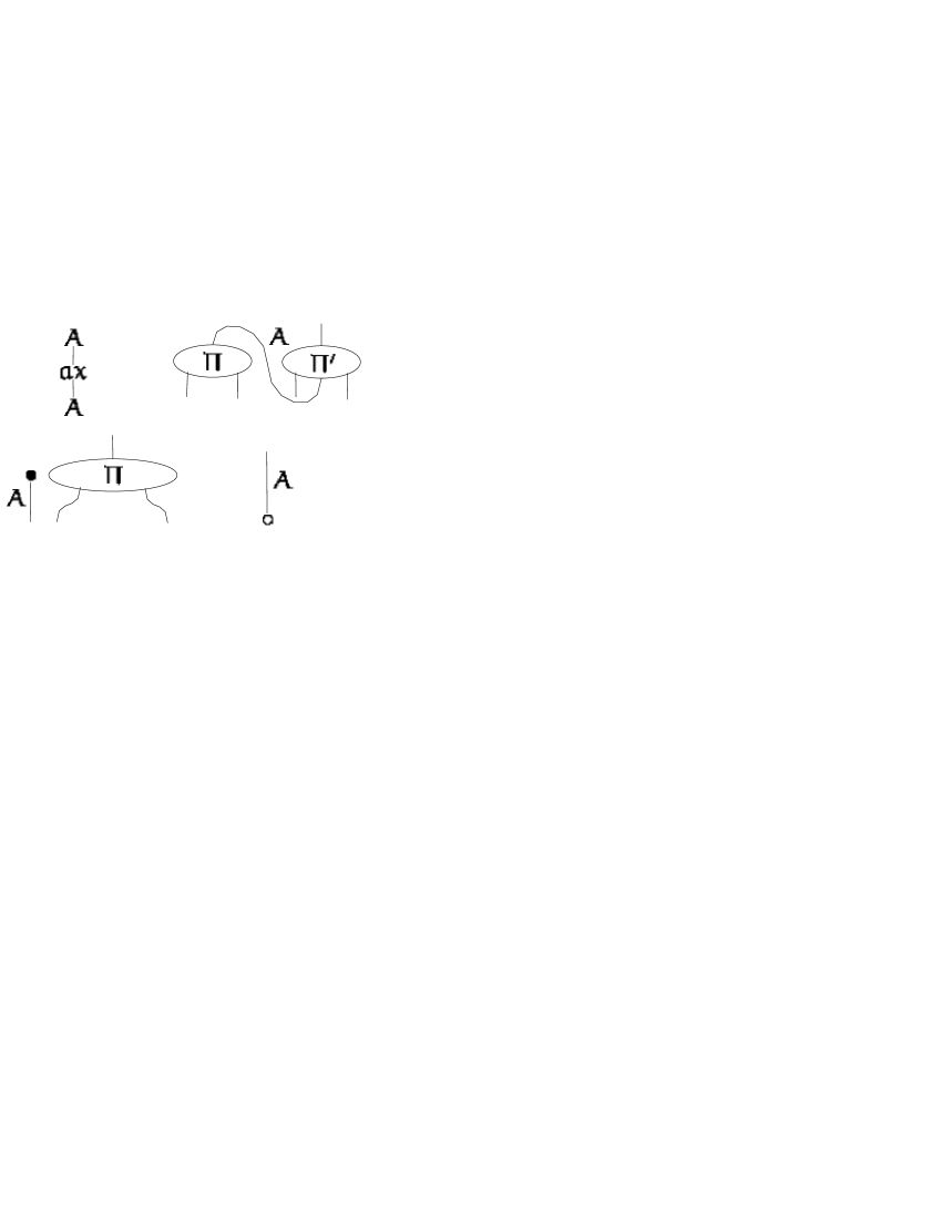
Figure 6. PNs of ILAL: axiom, cut, weakening, and unit

7,

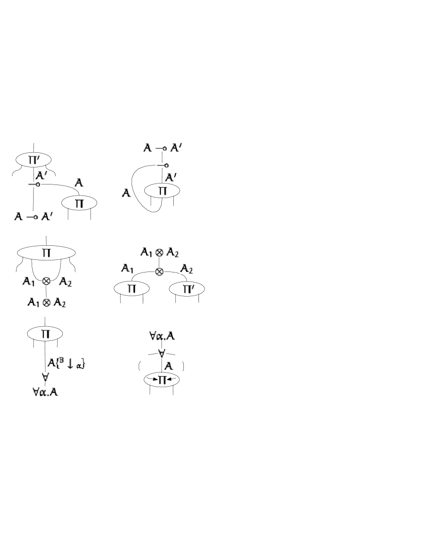
Figure 7. PNs of ILAL: the second order and multiplicative fragment

and 8.

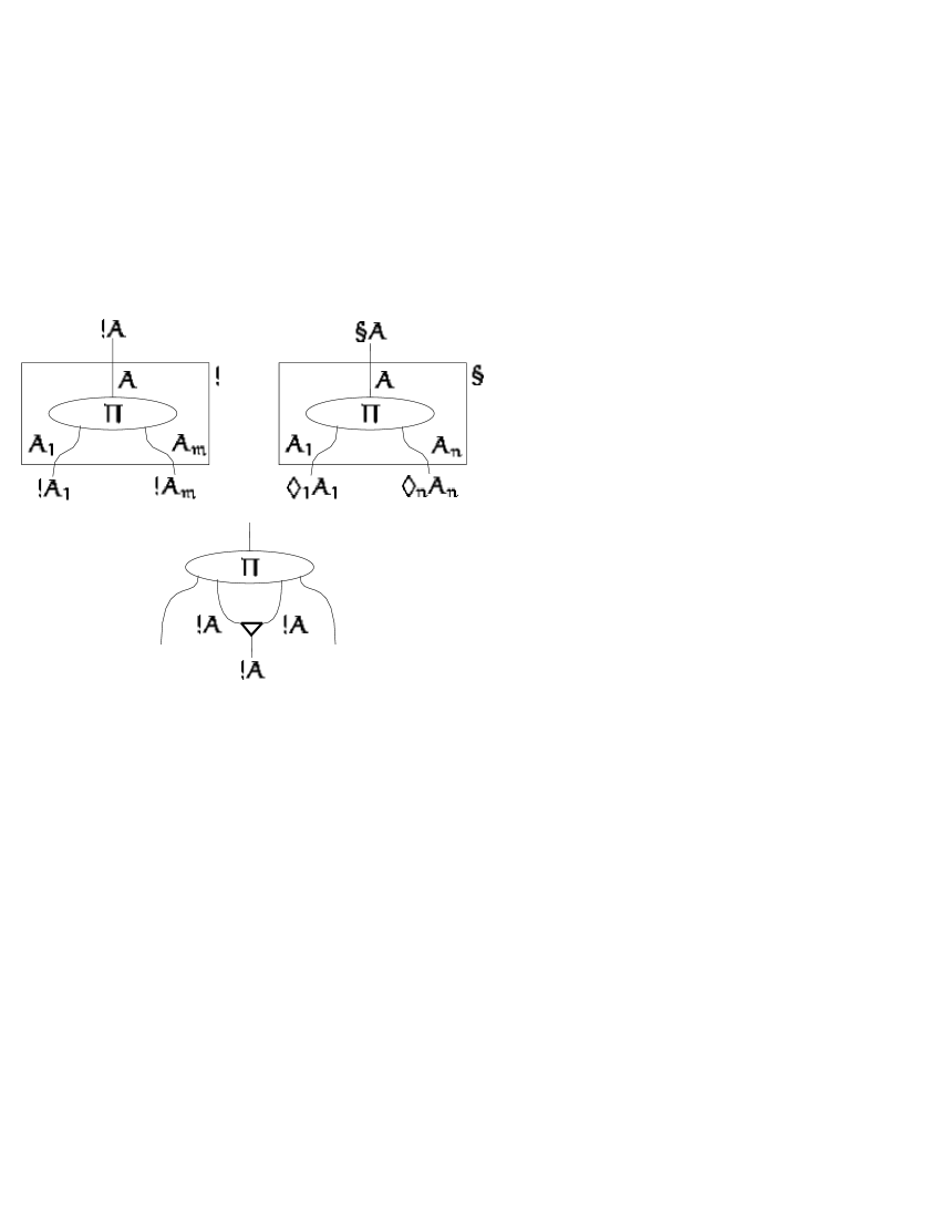
Figure 8. PNs of ILAL: the polynomial fragment

The PNs have a single output, and as many inputs as needed, possibly none. The output, also called root, is the link on top of the graph. The inputs, also called assumptions, are all the other links.

Figure 6 introduces the axiom , the cut, the weakening and the unit. The axiom, labeled $ax$, is a PN with a single input and a single output. If $\Pi$ and $\Pi^{\prime}$ are two PNs, the first with its output labeled by $A$, and the second with an input labeled by $A$, then the graph obtained by plugging the output of $\Pi$ into the input of $\Pi^{\prime}$ is a PN. With more traditional terminology, this is cutting the conclusion of $\Pi$ with the assumption of $\Pi^{\prime}$. Take again a PN $\Pi$. By putting a wire with a single input and no conclusions at all aside $\Pi$ yields a new PN: this is traditional weakening. Observe that the new, fake assumption is labeled by any formula $A$, namely, unlike traditional Linear logic, ILAL has an unconstrained weakening. Finally, the unit. It has a conclusion, but no inputs, like Linear logic’s unit $\mathbf{1}$. However, any formula can label our unit, and not only $\mathbf{1}$. Our unit serves to close the set of PNs with respect to the cut elimination, in presence of the unconstrained weakening.

Figure 7 defines the PNs for the second order and multiplicative fragment of ILAL. Everything is quite standard. Assume $\Pi$ and $\Pi^{\prime}$ be two PNs. Then, a new PN is obtained by wiring the conclusions/assumptions of $\Pi$/$\Pi^{\prime}$ as depicted. The introduction of a new root in the proof nets stands for an introduction to the right in sequent calculus terminology, while a new input is like an introduction to the left of the sequent calculus. Notice the $\forall$-introduction to the right (the lower-rightmost PN) in Figure 7. Its dashed links must point to all the wires of $\Pi$ whose labeling formula has $\alpha$ among its free variables. Moreover, no input wire of $\Pi$ must be pointed by the dashed links. This is like the usual $\forall$-introduction to the right: it requires that the variable being universally quantified is not a free variables of the assumptions. Our $\forall$-introduction to the right is not like in standard PNs of Linear logic. The standard construction, by means of a box, introduces an artificial sequentialization in the construction of the PNs that requires the use of commuting conversions to get the cut elimination. Our construction has not this drawback, simplifying the estimation of the cut elimination complexity.

Figure 8 defines the PNs for the polynomial fragment of ILAL. Assume $\Pi$ be a PN. A new PN is obtained either by enclosing $\Pi$ into a box, or by contracting two of its inputs, labeled by a modal formula $!A$, into a single input, labeled by $!A$ as well. There are two kinds of boxes. Any $!$-box has at most one input, labeled by a $!$-modal formula. So, in Figure 8, $m\leq 1$. On the contrary, there are not restrictions on the inputs of the $\S$-box: every $\lozenge_{i}$ belongs to $\{!,\S\}$, and $n$ is any integer, possibly $0$. The big difference between the two boxes will be appreciated when defining the cut elimination: a $!$-box can be duplicated, but every $\S$-box cannot.

4. Cut Elimination on Proof Nets

The main rules for eliminating the cuts are in Figures 9, 10, and 11. Figure 12, 13, 14, and 15 complete the cut elimination with garbage collection steps. The cut elimination rewrites graphs into other graphs which are not necessarily Proof nets of ILAL, but this will not be armuful.

Figure 9, introduce the linear steps. Figure 10 introduces the shifting step, and Figure 10 the polynomial step. This terminology is related to the cost of eliminating the corresponding cuts. The garbage collection cost will not be accounted because its steps only destroy existing structure: this means that the cost will never be greater than the dimension of the net being reduced.

Figure 9

Figure 9. Cut elimination: the linear steps

defines the linear cut elimination $\triangleright_{l}=\triangleright_{\beta}\cup\triangleright_{\otimes}\cup\triangleright_{\forall}$. The steps $\triangleright_{\beta}$ and $\triangleright_{\otimes}$ describe how a pair of $\multimap$ or $\otimes$-nodes annihilate each other. The step $\triangleright_{\forall}$ annihilates two $\forall$-nodes and produces $\Pi^{\prime}$ from $\Pi$ by substituting $B$ for every free occurrence of $\alpha$ in the formulas that label the edges of $\Pi$, pointed to by the dashed links.

Figure 10

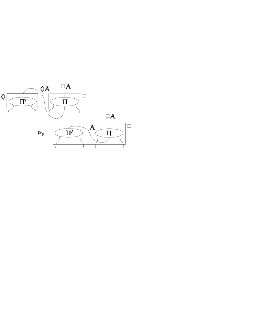
Figure 10. Cut elimination: the shifting step

defines the shifting cut elimination step $\triangleright_{s}$, which shifts a net $\Pi^{\prime}$, contained in a box, into another box. The $\Box$-box can be either a $\S$-box, or a $!$-box.

Figure 11 defines the rewriting relation $\triangleright_{p}$. It only duplicates $!$-boxes.

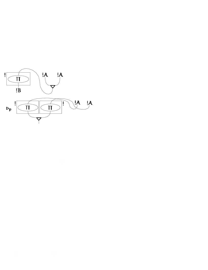
Figure 11. Cut elimination: the polynomial step

Figure 12

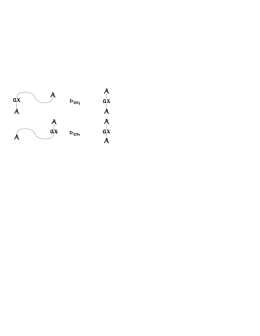
Figure 12. Cut elimination: the garbage collection generated by the axioms

the set of steps that compresses a sequence axiom/cut into a single axiom.

Figure 13

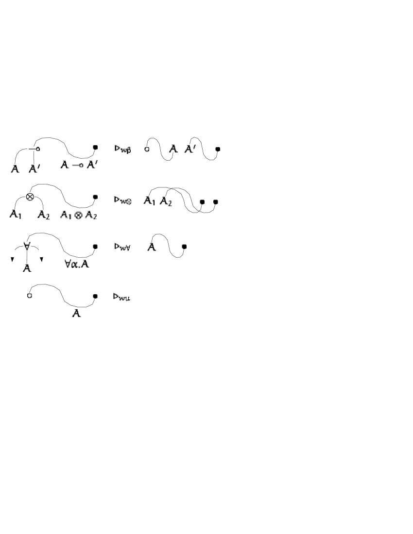
Figure 13. Cut elimination: the garbage collection generated by the unconstrained weakening

defines a second set of garbage collecting cut elimination steps. The use of the unconstrained weakening requires to consider all the possible configurations where the conclusion of some (sub-)net is plugged into the fake input of a weakening node. In such a case, the cut elimination proceeds just by erasing structure. In particular, for preserving the structural invariance that a cut link plugs the conclusion of a (sub-)net into the assumption of another (sub-)net, $\triangleright_{w\beta}$ introduces the unit net to erase the nodes of which the left link of the $\multimap$-node is an input. Figure 14

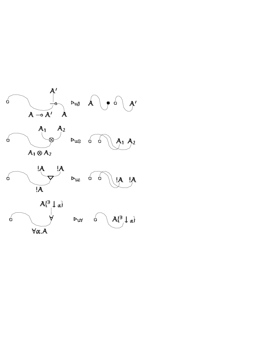
Figure 14. Cut elimination: the garbage collection generated by the unit

defines the garbage collecting cut elimination steps relative to our unit.

Finally, Figure 15

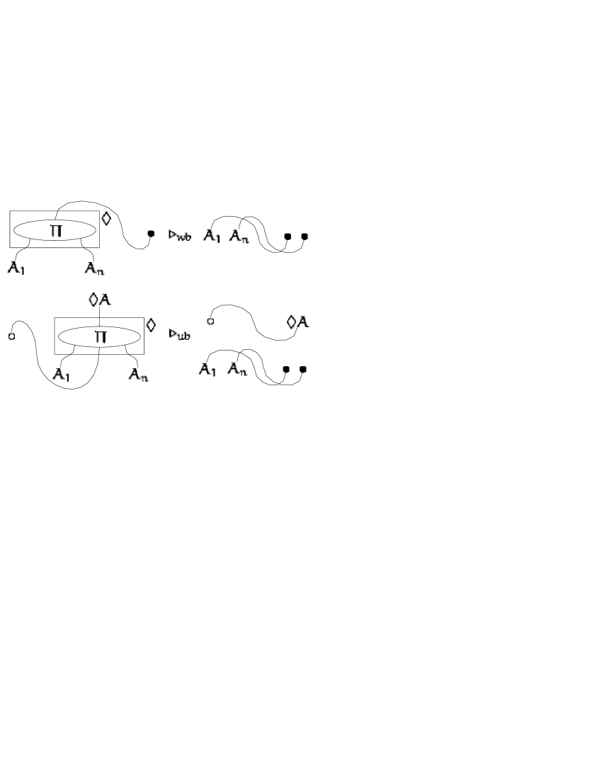
Figure 15. Cut elimination: the garbage collection generated erasing a box

shows what happens when erasing a box, using either a weakening or a unit. In particular, notice that $\triangleright_{wu}$ erases a box from the bottom: so the unit keeps erasing from $\lozenge A$ upward, while the weakening go downward.

We call $\triangleright_{l}$-normal a net $\Pi$ without $\triangleright_{l}$-redexes. We shall also use the analogous terminology for $\triangleright_{s}$ and $\triangleright_{p}$. If a net does not contain redexes of $\triangleright\equiv\triangleright_{l}\cup\triangleright_{s}\cup\triangleright_{p}$ it is simply normal. Of course, a net can also be garbage collected, so it is normal with respect to the rules in Figure 12 through 15. However we shall not pay very much attention to the garbage collection, when concerned to the complexity of the cut elimination. Ideed, the garbage collection can be “runned” at any instant without significant overhead: it strictly decreases the amount of existing structure.

4.1. Properties of the cut elimination

We observed that $\triangleright$ rewrites graphs into graphs and not Proof nets into Proof nets. This is not a problem:

Proposition 1.

The set of Proof nets for ILAL is closed under $\triangleright$.

This can be proved in few steps. The Proof nets of ILAL, without units and weakenings, can be embedded into those of functorial ILL, whose characterizing rules are recalled in Figure 16.

$$(!)\ \frac{\displaystyle A_{1},\ldots,A_{n}\vdash B}{\displaystyle!A_{1},\ldots,!A_{n}\vdash!B}$$

$$(Dereliction)\ \frac{\displaystyle\Gamma,A\vdash B}{\displaystyle\Gamma,!A\vdash B}$$

$$(Digging)\ \frac{\displaystyle\Gamma,!!A\vdash B}{\displaystyle\Gamma,!A\vdash B}$$

Figure 16. Functorial ILL: characterizing rules

The only point worth specifying on the embedding is that it maps every occurrence of $\S$ into an occurrence of $!$; the rest is a one-one correspondence. The closure extends to the whole language of ILAL Proof nets for some simple reasons. One of the two nets involved in the garbage collecting cut eliminations is always an unconnected component: either a unit or a weakening. Unit does not have inputs, so it does not create any problems concerning the construction order inherent to an inductive definition: given any net $\Pi$, we can always take a unit and cut its conclusion with any assumption of $\Pi$, with compatible type. Weakenings behave almost analogously. A weakening is always associated to some well formed net $\Pi$. Suppose that the elimination of a cut between a weakening and the root of a net $\Pi^{\prime}$ yields new cuts between the roots of the sub-nets of $\Pi^{\prime}$ and some weakenings. Then the newly generated weakenings can be thought of as introduced in association with $\Pi$ itself.

The Proof nets of ILAL are also a good computational language:

Proposition 2.

$\triangleright$ is Church-Rosser.

Start, again, from the Proof nets of ILAL, without units and weakenings, and embed them into those of functorial ILL. The strong normalizability of functorial ILL implies the same property for the considered fragment of ILAL. As we alrady observed, the garbage collection certainly does not break the strong normalizability, because it strictly decrease the size of the nets. Now, to check that Church-Rosser holds, just verify that the few critical pairs of $\triangleright$ are confluent. By the way, the critical pairs are the same as those of the Proof nets for (functorial) ILL.

5. P-Time Correctness

P-Time correctness means that, for any proof net $\Pi$, the number of cut links that must be eliminated to get to the normal form of $\Pi$ is bound by a polynomial in the dimension of $\Pi$.

This is the statement we shall prove by the end of this section.

It will turn out that the bound is:

$$O(\boldsymbol{D}^{3^{\boldsymbol{\partial}}}(\Pi))\enspace,$$

where $\boldsymbol{D}(\Pi)$ is the dimension of $\Pi$, and $\boldsymbol{\partial}$ is the maximal depth of $\Pi$. The dimension is, essentially, the number of nodes in $\Pi$. The depth of $\Pi$ is a purely structural property of $\Pi$, and will be introduced in a few.

The main tool to develop the proof of P-Time correctness is to find a measure that describes how $\boldsymbol{D}(\Pi)$ changes, as the cut elimination proceeds. Indeed, the number of nodes in a net always bound the number of the cut links that can be eliminated.

5.1. Proving P-Time Correctness

Every net can be stratified in levels:

Definition 1 (Level of a net).

For any net $\Pi$, a node of $\Pi$ is at level $l$ if it is enclosed into $l$ boxes of kind $!$ and/or $\S$.

The maximal depth of $\Pi$ is $\boldsymbol{\partial}(\Pi)$, or simply $\boldsymbol{\partial}$, if no ambiguity can exist.

Definition 2 (Dimensions of a Net).

Let $\Pi$ be a net, and $l\leq\boldsymbol{\partial}$.

• The dimension $d_{l}(\Pi)$ of $\Pi$ at level $l$ is the number of $\forall$, contraction nodes, $!$-boxes, and $\S$-boxes, plus $\multimap$ and $\otimes$-nodes, introduced either to the left, or to the right, at level $l$.

• The level-by-level dimension of $\Pi$ is:

  $$\mu(\Pi) = \langle d_{0}(\Pi),\ldots,d_{i}(\Pi),\ldots,d_{\boldsymbol{\partial}}(\Pi)\rangle$$

• The maximal dimension $\boldsymbol{D}(\Pi)$ is simply $\sum_{l=0}^{\boldsymbol{\partial}}d_{l}(\Pi)$.

Of course, when there are not ambiguities, the argument $\Pi$ is omitted.

• Remark.

  • The nodes at the same level $l$ can be “spread” in various boxes, each contributing to form the level $l$.

  • The space of tuples which $\mu$ belongs to is a well founded order, under the lexicographic relation $\succeq$. In particular, $\succ$ is the non reflexive part of $\succeq$.

Every point of a given net $\Pi$ can be taken as the root of a weighted sub-net:

Definition 3 (Weight of a Net).

Let $\Pi$ be a net. The weight $\operatorname{wgt}(\Pi)$ of $\Pi$ is a partial function from points of $\Pi$ to integers. If $a$ is any point on a link of $\Pi$:

$$\operatorname{wgt}(\Pi)(a) = 0\text{ with $a$ as in Figure~{}\ref{figure:weight-for-sub-nets-1st-case}, where}$$

$$\Box\in\{!,\S\} ax \Pi$$, and the -link is an input of

$$\operatorname{wgt}(\Pi)(a) = \operatorname{wgt}(\Pi)(b)\text{ with $a$, and $b$ as in Figure~{}\ref{figure:weight-for-sub-nets-2nd-case}}$$

$$\operatorname{wgt}(\Pi)(a) = \operatorname{wgt}(\Pi)(b)+1\text{ with $a$, and $b$ as in Figure~{}\ref{figure:weight-for-sub-nets-3rd-case}}$$

$$\operatorname{wgt}(\Pi)(a) = 1\text{ with $c$ as in Figure~{}\ref{figure:weight-for-sub-nets-3rd-case}}$$

$\operatorname{wgt}(\Pi)$ is undefined on any other point.

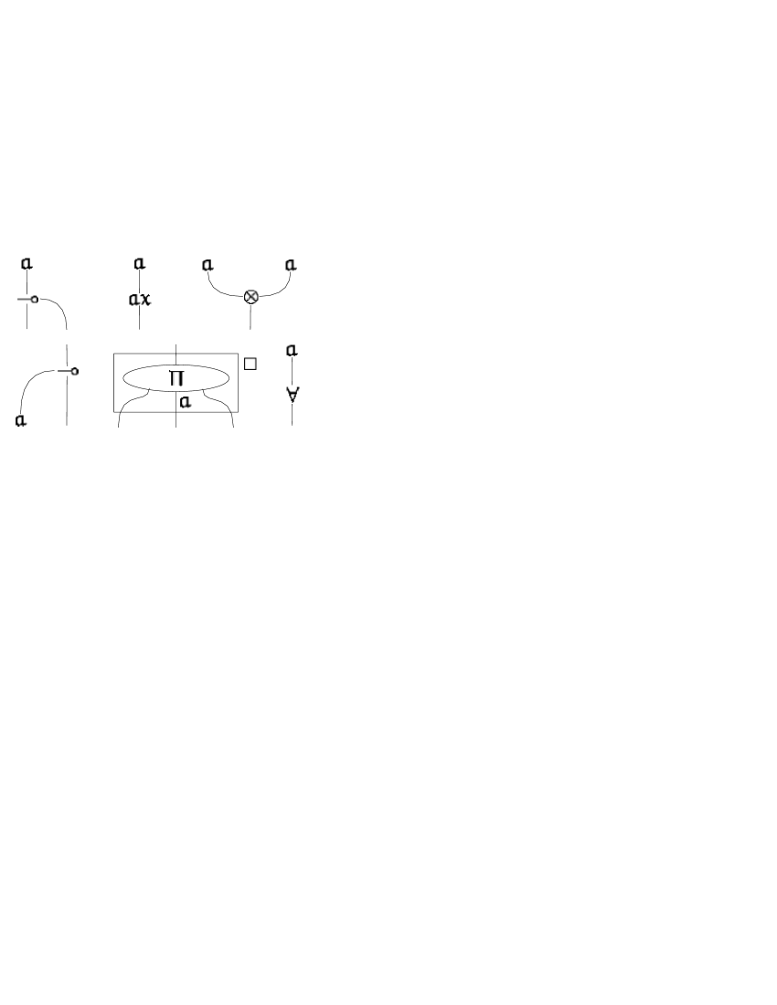
Figure 17. The weight of the sub-nets: first case

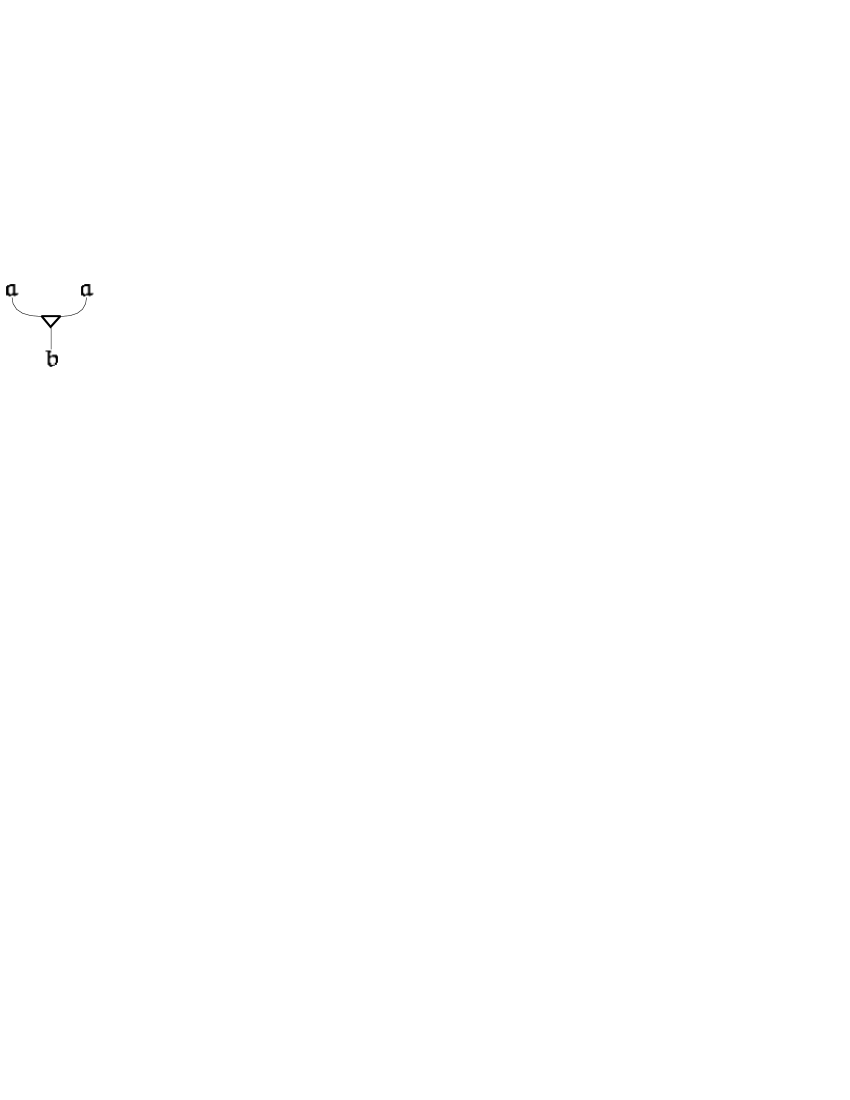
Figure 18. The weight of the sub-nets: second case

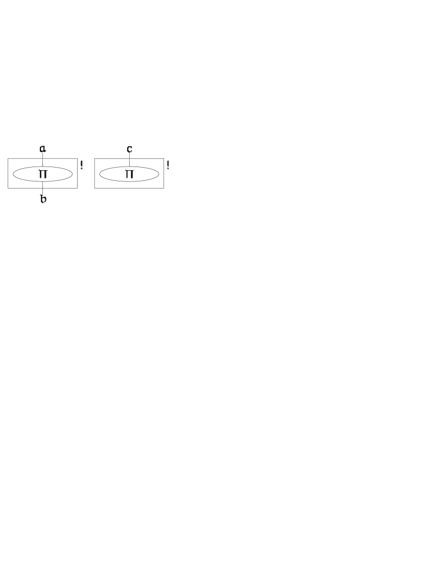
Figure 19. The weight of the sub-nets: third case

Definition 4 (Weight of a Contraction).

The weight $\operatorname{wgt}(\nabla)$ of any instance $\nabla$ of a contraction node in a net $\Pi$ is $\operatorname{wgt}(\Pi)(a)$ if $a$ labels the input of $\nabla$.

• Remark.

  • $\operatorname{wgt}(\nabla)$ is the number of $!$-boxes that can be duplicated by $\nabla$, and that are at the same level as $\nabla$ is at;

  • the points whose $\operatorname{wgt}$ is $0$ are those where a contraction node stops moving down, through a net, during the cut elimination;

  • every contraction node is as “heavy” as the weight of the net rooted at its input;

  • last, but not at all least, $\operatorname{wgt}$ is finite at every level, because the nets are defined inductively, and the cut elimination preserves their inductive structure.

Definition 5 (“Refined” Dimension of a Net).

Let $\Pi$ be a given net, and $l$ any integer of $\mathbb{Z}$.

• $n_{l}(\Pi)$ is the number of nodes $\forall$ plus the $\multimap$, and the $\otimes$-nodes, introduced either to the left, or to the right, at level $l$ in $\Pi$;

• $c^{w}_{l}(\Pi)$ is the number of contraction nodes at $l$ in $\Pi$ with weight $w$;

• $b_{l}(\Pi)$ is the total number of $!$-boxes, and $\S$-boxes at $l$ in $\Pi$;

• $\boldsymbol{W}_{l}(\Pi)$ is the maximal weight of the contraction nodes at $l$ in $\Pi$.

In particular, each of the quantities here above can assume any value in $\mathbb{N}$ if $0\leq l\leq\boldsymbol{\partial}(\Pi)$. Otherwise, their value can only be $0$.

When clear from the context, we omit $\Pi$, and also the level $l$.

The complexity bound follows from using a specific reduction strategy. The next definitions, and lemmas will serve to introducing such a strategy.

Definition 6 (Normalizing Measure of a Net).

For any net $\Pi$, its cut measure at level $0\leq l\leq\boldsymbol{\partial}$ is:

$$\gamma_{l}(\Pi) = \langle c^{\boldsymbol{W}_{l-1}}_{l-1},\ldots,c^{1}_{l-1},b_{l-1},n_{l}\rangle$$

• Remark.

  • The measure involves two levels of the net. If $l=0$, by Definition 5, the rightmost component can assume any natural value. All the others are $0$.

  • The space of tuples which $\gamma$ belongs to is a well founded order, under the lexicographic relation $\succeq$.

Definition 7 ($l$-normal Net).

Let $\Pi$ be a net, and $l\leq\boldsymbol{\partial}$. We say that $\Pi$ is $l$-normal when:

• $\Pi$ is $\triangleright_{l}$-normal at every level $0\leq i\leq l$, and

• $\Pi$ is $\triangleright_{s}\cup\triangleright_{p}$-normal at all levels $0\leq i\leq l-1$.

Fact 1.

If $\Pi$ is $\boldsymbol{\partial}$-normal, then $\Pi$ is, in fact, normal.

$\boldsymbol{\partial}$-normality means no $\triangleright_{l}$-redexes at any level, and no $\triangleright_{s}\cup\triangleright_{p}$-redexes at all levels but $\boldsymbol{\partial}$. Assuming the existence of a $\triangleright_{s}\cup\triangleright_{p}$-redex at $\boldsymbol{\partial}$, means to have some $!$ or $\S$-box at $\boldsymbol{\partial}$, against the definition of $\boldsymbol{\partial}$ for $\Pi$.

Fact 2.

Let $\Pi$ be $l-1$-normal, with $l\leq\boldsymbol{\partial}$, and such that $\Pi\triangleright_{l}\Pi^{\prime}$ by reducing a redex at $l$. Then:

(2) $$\gamma_{l}(\Pi)=\langle\ldots,n_{l}\rangle \succ \langle\ldots,n_{l}-1\rangle=\gamma_{l}(\Pi^{\prime})$$

(3) $$\mu(\Pi)=\langle\dots,d_{l},\ldots\rangle \succ \langle\dots,d_{l}-1,\ldots\rangle=\mu(\Pi^{\prime})$$

(2) holds because the reduction of a $\triangleright_{l}$-redex at level $l$ erases one node among $\forall,\multimap,\otimes$. So, (3) simply follows from (2).

Fact 3.

Let $\Pi$ be $l-1$-normal, with $l\leq\boldsymbol{\partial}$, and such that $\Pi\triangleright_{s}\Pi^{\prime}$ by reducing a redex at $l-1$. Then:

$$\gamma_{l}(\Pi)=\langle\ldots,b_{l-1}(\Pi),n_{l}(\Pi)\rangle\succ$$

$$\qquad\qquad\langle\ldots,b_{l-1}(\Pi)-1,n_{l}(\Pi)\rangle=\gamma_{l}(\Pi^{\prime})$$

$$\mu(\Pi)=\langle\ldots,d_{l-1}(\Pi),d_{l}(\Pi),\ldots\rangle\succ$$

$$\qquad\qquad\langle\ldots,d_{l-1}(\Pi)-1,d_{l}(\Pi),\ldots\rangle=\mu(\Pi^{\prime})\enspace.$$

Fact 3 is obvious for the reduction merges the border of two boxes, so decreasing their number at $l-1$.

Fact 4.

Let $\Pi$ be $l-1$-normal, with $l\leq\boldsymbol{\partial}$, and such that $\Pi\triangleright_{p}\Pi^{\prime}$ by eliminating a cut at $l-1$, which involves a contraction node $\nabla$ with weight $w\leq\boldsymbol{W}_{l-1}(\Pi)$. Then:

$$\gamma_{l}(\Pi) = \langle\ldots,c^{w}_{l-1}(\Pi),c^{w-1}_{l-1}(\Pi),\ldots,b_{l-1}(\Pi),n_{l}(\Pi)\rangle$$

$$\succ \langle\ldots,c^{w}_{l-1}(\Pi)-1,c^{w-1}_{l-1}(\Pi^{\prime}),\ldots,b_{l-1}(\Pi^{\prime}),n_{l}(\Pi^{\prime})\rangle$$

$$= \gamma_{l}(\Pi^{\prime})$$

$$\mu(\Pi) = \langle\ldots,d_{l-1}(\Pi),d_{l}(\Pi),\ldots,d_{\boldsymbol{\partial}}(\Pi),\rangle$$

$$\prec \langle\ldots,d_{l-1}(\Pi^{\prime}),d_{l}(\Pi^{\prime}),\ldots,d_{\boldsymbol{\partial}}(\Pi^{\prime}),\rangle$$

$$= \mu(\Pi^{\prime})$$

where:

(8) $$c^{w-1}_{l-1}(\Pi^{\prime}) \leq c^{w-1}_{l-1}(\Pi)+1$$

(9) $$b_{l-1}(\Pi^{\prime}) = b_{l-1}(\Pi)+1$$

(10) $$n_{l}(\Pi^{\prime}) \leq n_{l}(\Pi)+n_{l}(\Pi)$$

(11) $$d_{l-1}(\Pi^{\prime}) = d_{l-1}(\Pi)+1$$

(12) $$d_{l}(\Pi^{\prime}) \leq d_{l}(\Pi)+d_{l}(\Pi)$$

where $l\leq i\leq\boldsymbol{\partial}$.

(8) holds because $\nabla$ may be propagated below the just duplicated bos. In such a case, the weight decreases by one. (9) holds because the duplication introduces a $!$-box more than those in $\Pi$ at $l-1$. From this, it is obvious (11) as well. (10) holds because the introduction of a new $!$-box at level $l-1$ means to make one copy of at most all the nodes $\forall,\multimap$, and $\otimes$ at level $l$ of $\Pi$. This gives meaning also to (12).

Proposition 3.

Let $\Pi$ be $l-1$-normal, where $l\leq\boldsymbol{\partial}$. Assume that $\Pi$ rewrites to $\Pi^{\prime}$ by eliminating all $\triangleright_{p}$-cuts at level at $l-1$. Then, $\triangleright_{p}$ is strongly normalizable, and strongly confluent.

Strong normalizability trivially follows from Fact 4. Strong confluence follows from the absence of critical pairs in $\triangleright_{p}$.

Proposition 4.

Let $\Pi$ be $l-1$-normal, without $\triangleright_{p}$-redexes at level $l-1$, where $l\leq\boldsymbol{\partial}$. Assume that $\Pi$ rewrites to $\Pi^{\prime}$ by eliminating all $\triangleright_{s}$-cuts at level at $l-1$, and all $\triangleright_{l}$-redexes at level $l$, without assuming any precedence among the $\triangleright_{s}\cup\triangleright_{l}$-redexes. Then, $\triangleright_{s}\cup\triangleright_{l}$ is strongly normalizable, and strongly confluent.

Strong normalizability follows from Fact 2, and 3. Both imply that $\gamma$, and $\mu$ have a common upper bound as the elimination of $\triangleright_{s}\cup\triangleright_{l}$-redexes proceeds. Strong confluence follows from the absence of critical pairs in $\triangleright_{s}\cup\triangleright_{l}$.

The two, just given, properties support the definition of a reduction strategy:

Definition 8 (Cut Elimination Strategy).

Let $\Pi$ be $l-1$-normal. The cut elimination strategy $\triangleright_{\sigma}$ reduces redexes of $\triangleright_{l}\cup\triangleright_{s}\cup\triangleright_{p}$ in the following order:

• firstly, all the $\triangleright_{p}$-redexes at $l-1$,

• secondly, all the $\triangleright_{s}$-redexes at $l-1$, and the $\triangleright_{l}$-redexes at $l$, in any order.

Then, $\triangleright_{\sigma}$ stops.

Proposition 5.

Let $\Pi$, and $\Pi^{\prime}$ be such that $\Pi$ is $l-1$-normal, and $\Pi\triangleright_{\sigma}\Pi^{\prime}$. Then:

1. $\Pi^{\prime}$ is $l$-normal;

2. $\Pi\triangleright_{\sigma}\Pi^{\prime}$ takes at most $6\cdot\boldsymbol{D}^{3}(\Pi)$ steps.

3. $d_{i}(\Pi^{\prime})\leq 6\cdot\boldsymbol{D}^{3}(\Pi)$, for all $l\leq i\leq\boldsymbol{\partial}$.

Proof.

The first point is true by definition of $\triangleright_{\sigma}$.

Let us focus on the second point. Assume that:

$$\gamma_{l}(\Pi) = \langle\overbrace{d_{l-1},0,\ldots,0}^{\boldsymbol{W}_{l-1}=d_{l-1}\text{ times}},d_{l-1},d_{l}\rangle\enspace.$$

$\gamma_{l}(\Pi)$ here above is the worst possible assumption with respect of the number of cut elimination steps, necessary to normalize $\Pi$ at level $l$, because:

• we assume that all the contraction nodes at $l-1$, i.e. as many as $d_{l-1}(\Pi)$, have maximal weight. We saw that the weight of a contraction node $\nabla$ is the maximal number of $!$-boxes at $l-1$ that $\nabla$ can duplicate. Forcefully, the $!$-boxes at $l-1$ can not be more than $d_{l-1}(\Pi)$. This defines as many leftmost components of $\gamma_{l}(\Pi)$ as $d_{l-1}(\Pi)$;

• we assume to have as many $!$/$\S$-boxes as possible at $l-1$, namely $d_{l-1}(\Pi)$, defining the second component of $\gamma_{l}(\Pi)$ from its right;

• we assume to have as many nodes as possible at $l$ in $\Pi$, namely $d_{l}(\Pi)$, defining the rightmost component of $\gamma_{l}(\Pi)$.

Then, we make the hypothesis that every contraction node, $!$-box, $\S$-box at $l-1$, and every node at $l$ contributes to form a redex. Finally, we apply $\triangleright_{\sigma}$, and we observe the behavior of $\gamma_{l}(\Pi)$:

$$\gamma_{l}(\Pi)$$

$$\equiv \langle d_{l-1},0,\ldots,0,d_{l-1},d_{l}\rangle$$

$$\ldots\text{after $1$ step of $\triangleright_{p}$, from $\Pi$}\ldots$$

$$\succ \langle d_{l-1}-1,1,\ldots,0,d_{l-1}+1,d_{l}+d_{l}\rangle$$

$$\ldots\text{after $i$ steps of $\triangleright_{p}$, from $\Pi$}\ldots$$

$$\succ \langle d_{l-1}-i,i,\ldots,0,d_{l-1}+i,d_{l}+i\cdot d_{l}\rangle$$

$$\ldots\text{after $d_{l-1}$ steps of $\triangleright_{p}$, from $\Pi$}\ldots$$

$$\succ \langle 0,d_{l-1},0,\ldots,0,d_{l-1}+d_{l-1},d_{l}+d_{l-1}\cdot d_{l}\rangle$$

$$\equiv \langle\underbrace{0,d_{l-1},0,\ldots,0}_{d_{l-1}},2\cdot d_{l-1},(1+d_{l-1})\cdot d_{l}\rangle$$

$$\ldots\text{after $j\cdot d_{l-1}$ steps of $\triangleright_{p}$, from $\Pi$}\ldots$$

$$\succ \langle\underbrace{\underbrace{0,\ldots,0}_{j},d_{l-1},0,\ldots,0}_{d_{l-1}},(j+1)\cdot d_{l-1},(1+j\cdot d_{l-1})\cdot d_{l}\rangle$$

$$\ldots\text{after $d^{2}_{l-1}$ steps of $\triangleright_{p}$, from $\Pi$}\ldots$$

$$\succ \langle\underbrace{0,\ldots,0}_{d_{l-1}},(d_{l-1}+1)\cdot d_{l-1},(1+d^{2}_{l-1})\cdot d_{l}\rangle$$

$$\ldots\text{after $(d_{l-1}+1)\cdot d_{l-1}+(1+d^{2}_{l-1})\cdot d_{l}$ of $\triangleright_{s}\cup\triangleright_{l}$-steps}\ldots$$

$$\succ \langle 0,\ldots,0\rangle$$

$$\equiv \gamma_{l}(\Pi^{\prime})\enspace,$$

for some $\Pi^{\prime}$. By all that means that we have just rewritten $\Pi$ to $\Pi^{\prime}$ after, at most, $d^{2}_{l-1}+(d_{l-1}+1)\cdot d_{l-1}+(1+d^{2}_{l-1})\cdot d_{l}\in d_{l}(\Pi)\cdot d^{2}_{l-1}(\Pi)\leq 2\cdot(\boldsymbol{D}(\Pi)+\boldsymbol{D}^{2}(\Pi)+\boldsymbol{D}^{3}(\Pi))\leq 6\cdot\boldsymbol{D}^{3}(\Pi)$ steps, since $d_{l}(\Pi)\leq\boldsymbol{D}(\Pi)$, for every $0\leq l\leq\boldsymbol{\partial}(\Pi)$.

Finally, the third point. If we find $\mu(\Pi^{\prime})$, we get $\boldsymbol{D}(\Pi^{\prime})$ as well, which is the sum of all the components of $\mu(\Pi^{\prime})$. Assume again to start from $\Pi$, and to rewrite it under $\triangleright_{\sigma}$. We have:

$$\mu(\Pi)$$

$$\equiv \langle d_{0},\ldots,d_{l-2},d_{l-1},d_{l},\ldots,d_{\boldsymbol{\partial}}\rangle$$

$$\ldots\text{after $1$ step of $\triangleright_{p}$, from $\Pi$}\ldots$$

$$\prec \langle d_{0},\ldots,d_{l-2},d_{l-1}+1,d_{l}+d_{l},\ldots,d_{\boldsymbol{\partial}}+d_{\boldsymbol{\partial}}\rangle$$

$$\ldots\text{after $i$ steps of $\triangleright_{p}$, from $\Pi$}\ldots$$

$$\prec \langle d_{0},\ldots,d_{l-2},d_{l-1}+i,d_{l}+i\cdot d_{l},\ldots,d_{\boldsymbol{\partial}}+i\cdot d_{\boldsymbol{\partial}}\rangle$$

$$\ldots\text{after $d_{l-1}$ steps of $\triangleright_{p}$, from $\Pi$}\ldots$$

$$\prec \langle d_{0},\ldots,d_{l-2},d_{l-1}+d_{l-1},d_{l}+d_{l-1}\cdot d_{l},\ldots,d_{\boldsymbol{\partial}}+d_{l-1}\cdot d_{\boldsymbol{\partial}}\rangle$$

$$\equiv \langle d_{0},\ldots,d_{l-2},2\cdot d_{l-1},(1+d_{l-1})\cdot d_{l},\ldots,(1+d_{l-1})\cdot d_{\boldsymbol{\partial}},\rangle$$

$$\ldots\text{after $j\cdot d_{l-1}$ steps of $\triangleright_{p}$, from $\Pi$}\ldots$$

$$\prec \langle d_{0},\ldots,d_{l-2},(j+1)\cdot d_{l-1},(1+j\cdot d_{l-1})\cdot d_{l},\ldots,(1+j\cdot d_{l-1})\cdot d_{\boldsymbol{\partial}}\rangle$$

(13) $$\ldots\text{after $d^{2}_{l-1}$ steps of $\triangleright_{p}$, from $\Pi$}\ldots$$

$$\prec \langle d_{0},\ldots,d_{l-2},(d_{l-1}+1)\cdot d_{l-1},(1+d^{2}_{l-1})\cdot d_{l},\ldots,(1+d^{2}_{l-1})\cdot d_{\boldsymbol{\partial}}\rangle$$

$$\equiv \mu(\bar{\Pi})\enspace,$$

for some $\bar{\Pi}$. At this point, $\bar{\Pi}$ can be normalized at levels $l-1$, and $l$ by reducing all $\triangleright_{s}\cup\triangleright_{l}$-redexes which simply erase structure. We can safely state that, after (at most) $(d_{l-1}+1)\cdot d_{l-1}+(1+d^{2}_{l-1})\cdot d_{l}$ $\triangleright_{s}\cup\triangleright_{p}$-steps, $\mu(\bar{\Pi})$ here above is a bound for $\mu(\Pi^{\prime})$. It implies the third point we want to prove. ∎

In a few we shall get the bound on the cut elimination complexity. Thanks to Proposition 5 we can observe that each step $\triangleright_{\sigma}$ in:

$$\Pi_{0}\triangleright_{\sigma}\ldots\triangleright_{\sigma}\Pi_{i}\triangleright_{\sigma}\Pi_{i+1}\triangleright_{\sigma}\ldots$$

rewrites $\Pi_{i}$ in $\Pi_{i+1}$ using at most $6\cdot\boldsymbol{D}^{3}(\Pi_{i})$. So, $\Pi_{i}$ is obtained after at most

(14) $$\sum_{k=0}^{i}6^{\frac{3^{k}-1}{2}}\cdot\boldsymbol{D}^{3^{k}}(\Pi_{0})$$

steps. Fact 1 assures that the reduction sequence here above can not be longer than $\boldsymbol{\partial}(\Pi_{0})$. In particular, it is shorter if some $\triangleright_{ws}$-redexes erase, at some point, all the boxes constituting the $\boldsymbol{\partial}$-level of $\Pi_{0}$. So, the upper limit of (14) is $\boldsymbol{\partial}(\Pi_{0})$, and we get:

$$\sum_{k=0}^{\boldsymbol{\partial}(\Pi_{0})}6^{\frac{3^{k}-1}{2}}\cdot\boldsymbol{D}^{3^{k}}(\Pi_{0}) \leq 6^{\frac{3^{\boldsymbol{\partial}(\Pi_{0})}-1}{2}}\cdot\sum_{k=0}^{3^{\boldsymbol{\partial}(\Pi_{0})}}\boldsymbol{D}^{k}(\Pi_{0})$$

$$\leq 6^{\frac{3^{\boldsymbol{\partial}(\Pi_{0})}-1}{2}}\cdot\frac{\boldsymbol{D}^{3^{\boldsymbol{\partial}(\Pi_{0})}+1}(\Pi_{0})-1}{\boldsymbol{D}(\Pi_{0})-1}$$

$$\in O(\boldsymbol{D}^{3^{\boldsymbol{\partial}}}(\Pi_{0}))\enspace.$$

6. The Concrete Syntax

Figure 20

$$\mathsf{p} ::= \mathtt{T_{variables}}\ \mid\ \mathsf{p}\!\otimes\!\mathsf{p}$$

Figure 20. The patterns for the concrete syntax

introduces the patterns of our concrete syntax. The set of patterns is ranged over by $\mathsf{P}$, while $\mathtt{T_{variables}}$ is ranged over by $x,y,w,z$.

Figure 21

$$M,N ::= \mathtt{T_{variables}}\mid\ (\lambda\mathsf{P}.M)\ \mid\ (MN)\ \mid\ M\!\otimes\!N\ \mid\ !M\ \mid\ \overline{!}M\ \mid\ \S M\ \mid\ \bar{\phantom{|}\S}M$$

Figure 21. The concrete syntax

defines the set $\Lambda$ of the functional terms which we take as concrete syntax.

For any pattern $x_{1}\!\otimes\!\ldots\!\otimes\!x_{n}$, the set ${\mathtt{FV}}(x_{1}\!\otimes\!\ldots\!\otimes\!x_{n})$ of its free variables is $\{x_{1},\ldots,x_{n}\}$. As usual, $\lambda$ binds the variables of $M$ so that ${\mathtt{FV}}(\lambda\mathsf{P}.M)$ is ${\mathtt{FV}}(M)\setminus{\mathtt{FV}}(\mathsf{P})$. The free variable sets of all the remaining terms are obvious as the constructors $\otimes,!,\S,\overline{!}$, and $\bar{\phantom{|}\S}$ do not bind variables. Both $!$ and $\S$ build $!$-boxes and $\S$-boxes, respectively, being $M$ the body. The term constructor $\overline{!}$ can mark one of the entry points, namely the inputs, of both $!$-boxes, and $\S$-boxes, while $\bar{\phantom{|}\S}$ can mark only those of $\S$-boxes.

We shall adopt the usual shortening for $\lambda$-terms: $\lambda x_{1}.\ldots\lambda x_{n}.M$ is abbreviated by $\lambda x_{1}\ldots x_{n}.M$, and $(M_{1}\ldots(M_{n}N)\ldots)$ by $M_{1}\ldots M_{n}N$, i.e. the application is left-associative by default.

The elements of $\Lambda$ are considered up to the usual $\alpha$-equivalence. It allows the renaming of the bound variables of a term $M$. For example, $!(\lambda x.(\overline{!}y)\ x)$ and $!(\lambda z.(\overline{!}y)\ z)$ are each other $\alpha$-equivalent.

The substitution of $M$ for $x$ in $N$ is denoted by $N\{{}^{M}\!\downarrow{}_{x}\}$. It is the obvious extension to $\Lambda$ of the capture-free substitution of terms for variables, defined for the $\lambda$-Calculus. For example, $y\{{}^{x}\!\downarrow{}_{y}\}$ yields $y$.

The substitutions can be generalized to $\{^{M_{1}}\!\!\downarrow\!_{x_{1}}\cdots^{M_{n}}\!\!\downarrow\!_{x_{n}}\}$, which means the simultaneous replacement of $M_{i}$ for $x_{i}$, for every $1\leq i\leq n$.

We shall use $\equiv$ as syntactic coincidence.

7. The Type Assignment

We decorate the sequent calculus of Intuitionistic Light Affine Logic with the terms of the concrete syntax. So, the language of logical formulas and the sequent calculus we refer to are those in Figure 5.

Call basic set of assumptions any set of pairs $\{x_{1}:A_{1},\ldots,x_{n}:A_{n}\}$ that can be seen as a function with finite domain $\{x_{1},\ldots,x_{n}\}$. Namely, if $i\neq j$, then $x_{i}\neq x_{j}$.

An extended set of assumptions is a basic set, containing also pairs $\mathsf{P}:A$, that satisfies some further constraints. A pattern $\mathsf{P}\equiv x_{1}\!\otimes\!\ldots\!\otimes\!x_{m}:A$ belongs to an extended set of assumptions:

1. if $A$ is $A_{1}\!\otimes\!\ldots\!\otimes\!A_{p}$, with $p\geq m$, and

2. if $\{x_{1}:B_{1},\ldots,x_{m}:B_{m}\}$ is a basic set of assumptions, where every $B_{i}$ is either a single formula, or tensor of formulas.

For example, $\{x:\gamma,y:\beta\}$ is a legal extended set, while $\{z\!\otimes\!x:\gamma,y:\beta\}$ is not.

Talking about “assumptions”, we generally mean “extended set of assumptions”. Meta-variables for ranging over the assumptions are $\Gamma$, and $\Delta$.

The substitutions on formulas replace formulas for variables in the obvious way.

Figure 22

$$(Ax)\ \frac{\displaystyle}{\displaystyle x:B\vdash x:B}\qquad(Cut)\ \frac{\displaystyle\Gamma\vdash M:A\quad\Delta,x:A\vdash N:B}{\displaystyle\Gamma,\Delta\vdash N\{{}^{M}\!\downarrow{}_{x}\}:B}$$

$$(Weak.)\ \frac{\displaystyle\Gamma\vdash M:B}{\displaystyle\Gamma,x:A\vdash M:B}\qquad(Contr.)\ \frac{\displaystyle\Gamma,x:!A,y:!A\vdash M:B}{\displaystyle\Gamma,z:!A\vdash M\{{}^{z}\!\downarrow\!{}_{x}\ {}^{z}\!\downarrow\!{}_{y}\}:B}$$

$$(\multimap_{l})\ \frac{\displaystyle\Gamma\vdash M:A\qquad\Delta,y:B\vdash N:C}{\displaystyle\Gamma,\Delta,x:A\multimap B\vdash N\{{}^{xM}\!\downarrow{}_{y}\}:C} (\multimap_{r})\ \frac{\displaystyle\Gamma,\mathsf{P}:B_{1}\!\otimes\!\ldots\!\otimes\!B_{n}\vdash M:B}{\displaystyle\Gamma\vdash\lambda\mathsf{P}.M:B_{1}\!\otimes\!\ldots\!\otimes\!B_{n}\multimap B}$$

$$(\otimes_{l})\ \frac{\displaystyle\Gamma,x_{1}:B_{1},x_{2}:B_{2}\vdash M:B}{\displaystyle\Gamma,x_{1}\!\otimes\!x_{2}:B_{1}\!\otimes\!B_{2}\vdash M:B} (\otimes_{r})\ \frac{\displaystyle\Gamma\vdash M:B\quad\Delta\vdash N:A}{\displaystyle\Gamma,\Delta\vdash M\!\otimes\!N:B\!\otimes\!A}$$

$$(!)\ \frac{\displaystyle\ldots x_{i}:A_{i}\ldots\vdash M:B\qquad 0\leq i\leq n\leq 1}{\displaystyle\ldots x_{i}:!A_{i}\ldots\vdash!M\{\cdots{}^{\overline{!}x_{i}}\!\!\downarrow\!{}_{x_{i}}\cdots\}:!B}$$

$$(\S)\ \frac{\displaystyle\ldots x_{i}:B_{i}\ldots x^{\prime}_{j}:A_{j}\ldots\vdash M:B\qquad 0\leq i\leq m\quad 0\leq j\leq n}{\displaystyle\ldots x_{i}:!B_{i}\ldots x^{\prime}_{j}:\S A_{j}\ldots\vdash\S M\{\cdots{}^{\overline{!}x_{i}}\!\!\downarrow\!{}_{x_{i}}\cdots{}^{\bar{\phantom{|}\S}x^{\prime}_{j}}\!\!\downarrow\!{}_{x^{\prime}_{j}}\cdots\}:\S B}$$

$$(\forall_{l})\ \frac{\displaystyle\Gamma,x:\{{}^{B}\!\downarrow{}_{\alpha}\}A\vdash M:B}{\displaystyle\Gamma,x:\forall\alpha.A\vdash M:B} (\forall_{r})\ \frac{\displaystyle\Gamma\vdash M:A\qquad\alpha\not\in{\mathtt{FV}}(\Gamma)}{\displaystyle\Gamma\vdash M:\forall\alpha.A}$$

Figure 22. Decorating the sequent calculus with terms

introduces the sequent calculus of ILAL, decorated with the terms of $\Lambda$. Observe that $(!)$-rule can have at most one assumption. Observe also that the two rules for the second order formulas are not encoded by any term. Namely, we introduce a system analogous to Mitchell’s language Pure Typing Theory [Mit88]. In this case, the logical system of reference is second order ILAL, in place of System $\mathcal{F}$ [GLT89].

8. The Dynamics for the Concrete Syntax

Figure 23

$$(\lambda x_{1}\!\otimes\!\ldots\!\otimes\!x_{m\geq 1}.M)M_{1}\!\otimes\!\ldots\!\otimes\!M_{m}\ \rhd_{\beta} M\{^{M_{1}}\!\!\downarrow\!_{x_{1}}\cdots^{M_{m}}\!\!\downarrow\!_{x_{m}}\}$$

$$\overline{!}!M \rhd_{!} M$$

$$\bar{\phantom{|}\S}\S M \rhd_{\S} M$$

Figure 23. The rewriting relations for the concrete syntax

defines the basic rewriting relations on $\Lambda$.

The first relation is the trivial generalization of the $\beta$-rule of $\lambda$-Calculus to abstractions that bind patterns which represent tuples of variables. The $\alpha$-equivalence must be used to avoid variable clashes when rewriting terms. The second rewriting relation merges the borders of two boxes.

Define the rewriting system $\leadsto$ as the contextual closure on $\Lambda$ of the rewriting relations in Figure 23. Its reflexive, and transitive closure is $\leadsto^{*}$. The pair $(\Lambda,\leadsto)$ is the functional language we shall use to prove P-Time completeness of ILAL. We shall generally abuse the notation by referring to such a language only with $\Lambda$.

9. Comments on the Concrete Syntax

$\Lambda$ gives a very compact representation of the derivations. The contraction is represented by multiple occurrences of the same variable. The pattern matching avoids the use of any $let$-like binder that would require to extend $\leadsto$ by some commuting conversions. The boxes have not any interface like in the paradigmatic language proposals of [Asp98, Rov98, Rov00].

However, we have to pay for this notational economy. The typable sub-set of $\Lambda$ is not at all an isomorphic representation of the derivations. The simplest example to observe how ambiguously $\Lambda$ represents ILAL is in Figures 24,

$$(Contr.)\ \frac{\displaystyle(\S)\ \frac{\displaystyle x_{1}:!\alpha,x_{2}:!\alpha\vdash K\ x_{1}\ x_{2}:!\alpha}{\displaystyle w_{1}:!!\alpha,w_{2}:!!\alpha\vdash\S(K\ \bar{\phantom{|}\S}w_{1}\ \bar{\phantom{|}\S}w_{2}):\S!\alpha}}{\displaystyle z:!!\alpha\vdash\S(K\ \bar{\phantom{|}\S}z\ \bar{\phantom{|}\S}z):\S!\alpha}$$

$$(\S)\ \frac{\displaystyle(Contr.)\ \frac{\displaystyle x_{1}:!\alpha,x_{2}:!\alpha\vdash K\ x_{1}\ x_{2}:!\alpha}{\displaystyle w:!\alpha\vdash K\ w\ w:!\alpha}}{\displaystyle z:!!\alpha\vdash\S(K\ \bar{\phantom{|}\S}z\ \bar{\phantom{|}\S}z):\S!\alpha}$$

Figure 24. Two derivations for the same term

and 25.

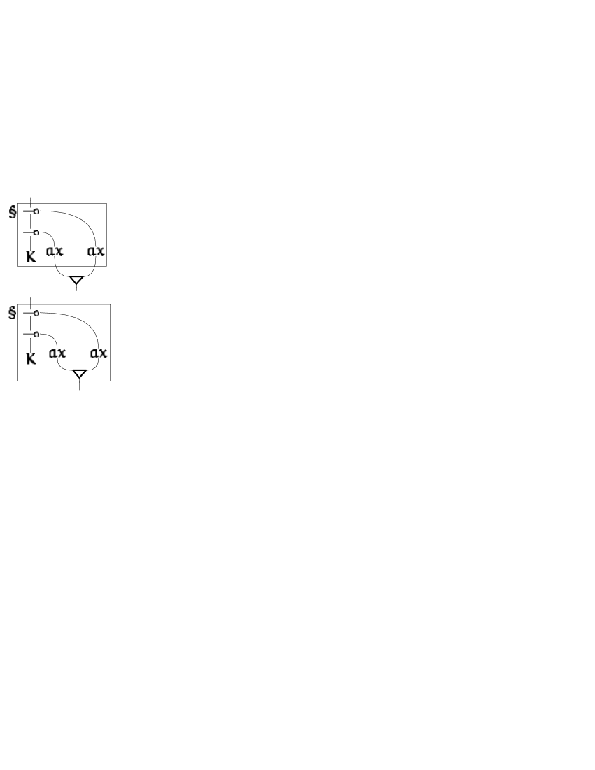
Figure 25. Two nets for the same term

The same term $\S(K\ \bar{\phantom{|}\S}z\ \bar{\phantom{|}\S}z)$ “encodes” two radically different derivations of the sequent calculus, i.e. $\S(K\ \bar{\phantom{|}\S}z\ \bar{\phantom{|}\S}z)$ “encodes”, under the same order as in Figure 24, the two nets in Figure 25.

Here we want to stress that such an ambiguity is not an issue for us. The concrete syntax is not meant to be a real calculus, but just a compact notation for proofs. What we need is a language where we can observe the type discipline at work, especially in the proof of P-Time completeness. In case we want to evaluate $M\in\Lambda$ with polynomial cost, the right way to do it is to translate $M$ into a proof net, so that $\triangleright_{\sigma}$ and the good computational properties of the nets can be exploited.

We only need to agree about the translation from $\Lambda$ to the nets. We choose the one putting the contractions as deeply as possible. So we would adopt the lower most net in Figure 25 as a translation of $\S(K\ \bar{\phantom{|}\S}z\ \bar{\phantom{|}\S}z)$. This choice reduces the computational complexity of the translation.

10. Encoding a Numerical System

The numerical system adopted on $\Lambda$ is the analogous of Church numerals for $\lambda$-Calculus.

The type and the terms of the tally integers are in Figure 26.

$$\boldsymbol{Int} = \forall\alpha.!(\alpha\multimap\alpha)\multimap\S(\alpha\multimap\alpha)$$

$$\overline{\mathit{0}} = \lambda x.\S\lambda y.y:\boldsymbol{Int}$$

$$\overline{n} = \lambda x.\S(\lambda y.\underbrace{\overline{!}x(\ldots(\overline{!}x}_{n}\ y)\ldots)):\boldsymbol{Int}\enspace.$$

Figure 26. The tally integers

Observe that there is a translation from $\Lambda$ to $\lambda$-Calculus that, applied to $\overline{\mathit{0}}$ and $\overline{n}$, yields $\lambda$-Calculus Church numerals:

$$\lambda fx.\underbrace{f(\ldots(f}_{n\geq 0}\ x)\ldots))\enspace.$$

The translation just erases all the occurrences of $!,\S,\overline{!}$, and $\bar{\phantom{|}\S}$.

Figure 27

$$\mathit{succ} = \lambda zx.\S(\lambda y.\overline{!}x(\bar{\phantom{|}\S}(z\ x)\ y)):\boldsymbol{Int}\multimap\boldsymbol{Int}$$

$$\mathit{sum} = \lambda wzx.\S(\lambda y.\bar{\phantom{|}\S}(w\ x)(\bar{\phantom{|}\S}(z\ x)\ y)):\boldsymbol{Int}\multimap\boldsymbol{Int}\multimap\boldsymbol{Int}$$

$$\mathit{iter} = \lambda xyz.\S(\bar{\phantom{|}\S}(x\ y)\ \bar{\phantom{|}\S}z):\boldsymbol{Int}\multimap!(A\multimap A)\multimap\S A\multimap\S A$$

$$\mathit{mult} = \lambda xy.\mathit{iter}\ x\ !(\lambda w.\mathit{sum}\ \overline{!}y\ w)\ \S\overline{\mathit{0}}:\boldsymbol{Int}\multimap!\boldsymbol{Int}\multimap\S\boldsymbol{Int}$$

$$\mathit{coerc} = \lambda x.\S(\bar{\phantom{|}\S}(x\ !\mathit{succ})\ \overline{\mathit{0}}):\boldsymbol{Int}\multimap\S\boldsymbol{Int}\enspace.$$

Figure 27. Some combinators on the tally integers

introduces some further combinators on the numerals. The numeral next to $\overline{n}$ can be calculated as in Figure 28.

$$\mathit{succ}\ \overline{n}$$

$$\leadsto \lambda x.\S(\lambda y.\overline{!}x(\bar{\phantom{|}\S}(\overline{n}\ x)\ y))$$

$$\leadsto \lambda x.\S(\lambda y.\overline{!}x(\bar{\phantom{|}\S}\S(\lambda w.\overbrace{\overline{!}x(\ldots(\overline{!}x}^{n}\ w)\ldots))\ y))$$

$$\leadsto \lambda x.\S(\lambda y.\overline{!}x((\lambda w.\overline{!}x(\ldots(\overline{!}x\ w)\ldots))\ y))$$

$$\leadsto \lambda x.\S(\lambda y.\underbrace{\overline{!}x(\overline{!}x(\ldots(\overline{!}x}_{n+1}\ y)\ldots)))$$

$$= \overline{n+1}\enspace.$$

Figure 28. Calculating the numeral next to $\overline{n}$

$\mathit{sum}$ adds two numerals. $\mathit{iter}$ takes as arguments a numeral, a step function, and a base where to start the iteration from. Observe that $\mathit{iter}\ \overline{2}\ !\overline{n}\ \S\overline{\mathit{0}}$ cannot have type, for any numeral $\overline{n}$. This because the step function is required to have identical domain and co-domain. This should not surprise. Taking the $\lambda$-Calculus Church numeral $\overline{2}$, and applying it to itself we get an exponentially costing computation.

$\mathit{mult}$ is defined as an iterated sum, for multiplying two numerals.

Finally, $\mathit{coerc}(\text{ion})$ embeds a numeral into a $\S$-box, preserving its value. Look at Figure 29 for an example.

$$\mathit{coerc}\ \overline{n}$$

$$\leadsto \S(\bar{\phantom{|}\S}(\overline{n}\ !\mathit{succ})\ \overline{\mathit{0}})$$

$$\leadsto \S(\bar{\phantom{|}\S}(\S(\lambda w.\overline{!}!\mathit{succ}(\ldots(\overline{!}!\mathit{succ}\ w)\ldots)))\ \overline{\mathit{0}})$$

$$\leadsto \S((\lambda w.\mathit{succ}(\ldots(\mathit{succ}\ w)\ldots)))\ \overline{\mathit{0}})$$

$$\leadsto \S(\overbrace{\mathit{succ}(\ldots(\mathit{succ}}^{n}\ \overline{\mathit{0}})\ldots))$$

$$\leadsto^{*} \S\overline{n}\enspace.$$

Figure 29. Coercion of $\overline{n}$ to $\S\overline{n}$

10.1. Encoding a Predecessor

The predecessor of the numerical system for $\Lambda$ is an instance of a general computation scheme that iterates the template function in Figure 30.

$$\mathcal{T}_{f}(g,h) = (f,gh)\enspace.$$

Figure 30. Template function for the predecessor

$\mathcal{T}$ takes a pair of functions $h,g$ as arguments, and has $f$ as its parameter. If $h:X\rightarrow Y,g:Y\rightarrow Z$, and $f:Z\rightarrow Z$, for some domains $X,Y,Z$, then $\mathcal{T}_{f}$ can be iterated. An example of an $n$-fold iteration of $\mathcal{T}_{f}$ from $(g,h)$ is in Figure 31,

$$\overbrace{\mathcal{T}_{f}(\ldots\mathcal{T}_{f}}^{n}(gh)\ldots) = (f,\overbrace{f(\ldots f}^{n-1}(gh)\ldots))$$

Figure 31. Iterating the template function

where it is simple to recognize the predecessor of $n$, if we let $f:\mathbb{N}\rightarrow\mathbb{N}$ be the identity, $g:\mathbb{N}\rightarrow\mathbb{N}$ be the successor, $h$ be $0$, and if we assume to erase the first component of the result. Recasting everything in $\Lambda$, we get the definitions in Figure 32.

$$I = \lambda x.x:\forall\alpha.\alpha\multimap\alpha$$

$$\pi_{2} = \lambda x\otimes y.y:\forall\alpha.\alpha\otimes\alpha\multimap\alpha$$

$$T = \lambda f.\lambda g\otimes h.(f\otimes(gh)):\forall\alpha.(\alpha\multimap\alpha)\multimap((\alpha\multimap\alpha)\otimes\alpha)\multimap(\alpha\multimap\alpha)\otimes\alpha$$

$$\mathit{step}\ z = T\ z:((\boldsymbol{Int}\multimap\boldsymbol{Int})\otimes\boldsymbol{Int})\multimap(\boldsymbol{Int}\multimap\boldsymbol{Int})\otimes\boldsymbol{Int}$$

$$\mathit{base}\ y = T\ I\ (I\otimes y):(\boldsymbol{Int}\multimap\boldsymbol{Int})\otimes\boldsymbol{Int}$$

$$\mathit{pred} = \lambda wx.\S(\lambda y.\pi_{2}(\bar{\phantom{|}\S}(w\ !(\mathit{step}\ \overline{!}x))(\mathit{base}\ y))):\boldsymbol{Int}\multimap\boldsymbol{Int}$$

where $$y,z:\boldsymbol{Int}$$

Figure 32. The predecessor

The term $\mathit{pred}$ iterates $w$ times $!(\mathit{step}\ \overline{!}x)$ from $I\otimes y$, exploiting the correspondence between $\mathcal{T}$ and $T$ in Figure 33.

$T$	$\mathcal{T}$
$!(\mathit{step}\ \overline{!}x)$	$f$
$I$	$g$
$I\!\otimes\!y$	$h$

Figure 33. Correspondence between $\mathcal{T}$ and $T$

Observe also that our predecessor does not make any explicit use of the encoding of the additive types by means of the second order quantification. In [Asp98] the predecessor has a somewhat more intricate form that we recall here:

(15) $$\lambda nxy.(n\ (\lambda p.(U\ I\ x\ (p\ \mathit{snd})))\ (U\ I\ I\ y)\ \mathit{fst})\enspace,$$

where:

$$U\ P\ Q\ R = \lambda z.(z\ P\ Q\ R)$$

$$\mathit{fst} = \lambda xyz.(x\ z)$$

$$\mathit{snd} = \lambda xyz.(y\ z)\enspace.$$

$\mathit{pred}$ is obtained by eliminating the non essential components of (15) here above.

Both $\mathit{pred}$, and (15) are syntactically linear, so also their complexity is readily linear. On the contrary, the usual encoding of the predecessor, that, using $\lambda$-Calculus syntax with pairs $\langle M,N\rangle$, is:

(16) $$\lambda nxy.\mathit{fst}(n\ (\lambda p.\langle\mathit{snd}(p),x\ \mathit{snd}(p)\rangle)\ \langle y,y\rangle)\enspace,$$

has also an exponential strategy. Such a strategy exists because the term is not syntactically linear. However both $\mathit{pred}$, and (15) witness that the non linearity of (16) is inessential. In particular, in [Gi98], where Girard embeds (16) in LLL, the sub-term $\lambda p.\langle\mathit{snd}(p),x\ \mathit{snd}(p)\rangle$ here above has the additive type $(\alpha\&\alpha)\multimap(\alpha\&\alpha)$. This means that, at every step of the iteration $n\ (\lambda p.\langle\mathit{snd}(p),x\ \mathit{snd}(p)\rangle)\ \langle y,y\rangle$, only one of the multiple uses of $p$ is effectively useful to produce the result.

• Remark.

  • The procedural iteration scheme in Figure 31, our predecessor is an instance of, was already used in [Rov98]. However, only reading [DJ99], we saw that the iteration in Figure 31 actually “implements” a general logical iteration scheme, which we adapt to ILAL in Figure 34. There, the term $M$ must contain $g\ h$, the argument of $n\ \mathcal{T}_{f}$.

    $$(\multimap_{l})\ \frac{\displaystyle!\Gamma\vdash\mathcal{T}_{f}:!(A\multimap A)\qquad\qquad\qquad\Delta,y:\S(A\multimap A)\vdash M:B}{\displaystyle(\forall_{l})\ \frac{\displaystyle!\Gamma,\Delta,n:(!(\alpha\multimap\alpha)\multimap\S(\alpha\multimap\alpha))\{{}^{A}\!\downarrow{}_{\alpha}\}\vdash M\{{}^{\bar{\phantom{|}\S}(n\ \mathcal{T}_{f})}\!\downarrow{}_{y}\}:B}{\displaystyle!\Gamma,\Delta,\boldsymbol{Int}\vdash M\{{}^{\bar{\phantom{|}\S}(n\ \mathcal{T}_{f})}\!\downarrow{}_{y}\}:B}}$$

    Figure 34. General iteration scheme: the logical structure

    The more traditional iteration scheme can be obtained from Figure 34 by letting $!\Delta,y:\S(A\multimap A)\vdash M:B$ be the conclusion of the derivation in Figure 35.

    $$(\multimap_{l})\ \frac{\displaystyle\Theta\vdash N:A\qquad\qquad x:A\vdash x:A}{\displaystyle(\S)\ \frac{\displaystyle\Theta,y:A\multimap A\vdash y\ N:A}{\displaystyle\S\Theta,w:\S(A\multimap A)\vdash\S(\bar{\phantom{|}\S}w\ N):\S A}}$$

    Figure 35. Getting the standard iteration scheme

    Observe that the instance of $M$ we use for our predecessor is not as simple as $\S(\bar{\phantom{|}\S}w\ N)$.

  • We want to discuss a little more about the linearity of the additive structures. Not sticking to any particular notation, let $fxy=\mathit{fst}\langle xy,xy\rangle$. The function $f$ is just the identity, and it would get a linear type in ILAL. Now, consider an $n$-fold iteration of $f$ by means of a Church numeral $\overline{n}$ . Then, let us apply the result to a pair of identities. We have just defined $g_{f}\ n=((n\ f)\ I)\ I$. This term is typable in ILAL. So, in ILAL, $g_{f}\ n$ normalizes in polynomial, actually linear, time. However, try to reduce $g_{f}\ n$ in most traditional lazy call-by-value implementations of functional languages (SML, CAML, Scheme, etc.), you will discover that the reduction takes exponential time. So, firstly, if a usual $\lambda$-term $M$ can be embedded in ILAL, then, in general, it is not true that $M$ normalizes in polynomial time under any reduction strategy. We only know that there exists an effective way to normalize $M$ in polynomial time. The polynomial reduction, in general, is not compatible with the lazy call-by-value reduction.

    However, consider again $g_{f}\ n=((n\ f)\ I)\ I$ and evaluate it under the lazy call-by-name strategy: it will cost linear time. We leave the following open question: is it true that, taking a typable term $M$ having a polynomial reduction strategy, then that strategy can be the lazy call-by-name?

11. Encoding the Polynomials

In this section we show how to encode the elements of $\mathcal{P}$, i.e. the polynomials with positive degrees, and positive coefficients, as terms of $\Lambda$. This encoding is based on the numerical system of Section 10. It will serve to represent and simulate all P-Time Turing machines using the terms of ILAL.

We use $p^{\vartheta}_{x}$ to range over the polynomials $\sum_{i=0}^{\vartheta}a_{i}x^{i}\in\mathcal{P}$ with maximal non null degree $\vartheta$, and indeterminate $x$.

The result of this section is:

Theorem 1.

There is a translation $\hat{\phantom{p}}:\mathcal{P}\rightarrow\Lambda$, such that, for any $p^{\vartheta}_{x}\in\mathcal{P}$:

• $\hat{p}^{\vartheta}_{x}:\boldsymbol{Int}\multimap\S^{\vartheta+3}\boldsymbol{Int}$, and

• $p^{\vartheta}_{n}=m$, if, and only if, $\hat{p}^{\vartheta}_{\overline{n}}\leadsto^{*}\S^{\vartheta+3}\overline{m}$.

In the following we develop the proof of the theorem, and an example about how the encoding works.

First of all, some useful notations.

Let $p^{\vartheta}_{x}$ be the polynomial $\sum_{i=0}^{\vartheta}a_{i}x^{i}$ describing the computational bound of the Turing machine being encoded. Let $\kappa=\frac{\vartheta(\vartheta+1)}{2}$.

Abbreviate with $\vec{y}_{n}$ an $n$-long vector of all vectors with length $1$ through $n$, each containing variables $y^{j}_{i}\in\mathtt{T_{variables}}$, where $0\leq i\leq n-1$, and $1\leq j\leq n$. Figure 36

$$\vec{y}_{3} = \begin{array}[t]{ccc}y^{1}_{0}&&\\ y^{2}_{0}&y^{2}_{1}&\\ y^{3}_{0}&y^{3}_{1}&y^{3}_{2}\end{array}$$

Figure 36. Vector of vectors of variables

gives $\vec{y}_{3}$ as an example. As usual, $\vec{y}_{3}[i][j]$ picks $y^{j}_{i}$ out of the vector $\vec{y}$.

Figure 37,

$$\boldsymbol{Int}_{n} = \boldsymbol{Int}\otimes\ldots\otimes\boldsymbol{Int}\qquad\text{with }n\text{ components}$$

$$\overline{0}_{n} = \overline{0}\otimes\ldots\otimes\overline{0}\qquad\qquad\text{with }n\text{ components}$$

$$\lozenge^{n}M = \underbrace{\lozenge(\ldots(\lozenge}_{n}M)\ldots)\qquad\text{with }\lozenge\in\{!,\S,\overline{!},\bar{\phantom{|}\S}\}$$

$$\overline{0}^{p,q} = \S^{p}!^{q}\overline{0}:\S^{p}!^{q}\boldsymbol{Int}$$

$$\mathit{sum}_{n} = \lambda x_{1}\!\otimes\!\ldots\!\otimes\!x_{n}z.\S(\lambda y.\bar{\phantom{|}\S}(x_{1}\ z)(\ldots(\bar{\phantom{|}\S}(x_{n}\ z)\ y)\ldots)):\boldsymbol{Int}_{n}\multimap\boldsymbol{Int}$$

$$\mathit{sum}^{p}_{n} = \lambda x_{1}\!\otimes\!\ldots\!\otimes\!x_{n}.\S^{p}(\mathit{sum}_{n}\ \bar{\phantom{|}\S}^{p}x_{1}\!\otimes\!\ldots\!\otimes\!\bar{\phantom{|}\S}^{p}x_{n}):(\S^{p}\boldsymbol{Int})_{n}\multimap\S^{p}\boldsymbol{Int}$$

$$\mathit{succ}^{p,q} = \lambda x.\S^{p}(!^{q}(\mathit{succ}\ \overline{!}^{q}(\bar{\phantom{|}\S}^{p}x))):\S^{p}!^{q}\boldsymbol{Int}\multimap\S^{p}!^{q}\boldsymbol{Int}$$

$$\mathit{coerc}^{p,q} = \lambda x.\S(\bar{\phantom{|}\S}(x\ !\mathit{succ}^{p,q})\ \overline{0}^{p,q}):\boldsymbol{Int}\multimap\S^{p+1}!^{q}\boldsymbol{Int}$$

$$\mathit{mult}^{p} = \lambda xy.\S^{p}(\mathit{mult}\ \bar{\phantom{|}\S}^{p}x\ \bar{\phantom{|}\S}^{p}y):\S^{p}\boldsymbol{Int}\multimap\S^{p}!\boldsymbol{Int}\multimap\S^{p+1}\boldsymbol{Int}$$

$$\mathit{tuple}_{n} = \lambda x.\S(\bar{\phantom{|}\S}(x\ !(\lambda x_{1}\!\otimes\!\ldots\!\otimes\!x_{n}.\mathit{succ}\ x_{1}\!\otimes\!\ldots\!\otimes\!\mathit{succ}\ x_{n}))\ \overline{0}_{n}):$$

$$\qquad\qquad\qquad\qquad\qquad\qquad\qquad\qquad\qquad\qquad\qquad\quad\boldsymbol{Int}\multimap\S(\boldsymbol{Int}_{n})$$

Figure 37. Generalizations of operations on the numerals

where $p,q\geq 0$, and $n\geq 1$, introduces both a type abbreviation, and some generalizations of the operations on Church numerals in Section 10.

Figure 38

$$\hat{p}^{\vartheta}_{x} = \lambda x.\S((\lambda\begin{array}[t]{l}y^{1}_{0}\\ \!\otimes\!\ldots\!\otimes\!\\ y^{i}_{0}\;\!\otimes\!\ldots\!\otimes\!y^{i}_{i-1}\\ \!\otimes\!\ldots\!\otimes\!\\ y^{\vartheta}_{0}\!\otimes\!\ldots\!\otimes\!y^{\vartheta}_{\vartheta-1}.\end{array}$$

$$\phantom{\lambda x.\S((}\mathit{sum}^{\vartheta+2}_{\vartheta+1}\ \S^{1}(\mathit{coerc}^{\vartheta,0}\ \bar{\phantom{|}\S}^{1}\langle\!\langle a_{0}x^{0}\rangle\!\rangle_{\vec{y}_{\vartheta}[0]})$$

$$\phantom{\lambda x.\S((\mathit{sum}^{\vartheta+1}_{\vartheta+1}\ }\qquad\qquad\vdots$$

$$\phantom{\lambda x.\S((\mathit{sum}^{\vartheta+1}_{\vartheta+1}\ }\!\otimes\!\S^{i+1}(\mathit{coerc}^{\vartheta-i,0}\ \bar{\phantom{|}\S}^{i+1}\langle\!\langle a_{i}x^{i}\rangle\!\rangle_{\vec{y}_{\vartheta}[i]})$$

$$\phantom{\lambda x.\S((\mathit{sum}^{\vartheta+1}_{\vartheta+1}\ }\qquad\qquad\vdots$$

$$\phantom{\lambda x.\S((\mathit{sum}^{\vartheta+1}_{\vartheta+1}\ }\!\otimes\!\S^{\vartheta+1}(\mathit{coerc}^{0,0}\ \bar{\phantom{|}\S}^{\vartheta+1}\langle\!\langle a_{\vartheta}x^{\vartheta}\rangle\!\rangle_{\vec{y}_{\vartheta}[\vartheta]})$$

$$\phantom{\lambda x.\S(})\ \bar{\phantom{|}\S}(\mathit{tuple}_{\kappa}\ x)):\boldsymbol{Int}\multimap\S^{\vartheta+3}\boldsymbol{Int}$$

where:

$$\langle\!\langle ax^{0}\rangle\!\rangle_{\vec{z}} \mapsto \mathit{coerc}^{0,0}\ \overline{a}:\S\boldsymbol{Int}$$

$$\langle\!\langle ax^{n}\rangle\!\rangle_{\vec{z}} \mapsto \mathit{mult}^{n}\ \langle\vec{z},n-1\rangle\ (\mathit{coerc}^{n-1,1}\ \overline{a}):\S^{n+1}\boldsymbol{Int}\qquad(n\geq 1)$$

$$\langle\vec{z},0\rangle \mapsto \mathit{coerc}^{0,0}\ \vec{z}[0]:\S\boldsymbol{Int}$$

$$\langle\vec{z},n\rangle \mapsto \mathit{mult}^{n}\ \langle\vec{z},n-1\rangle\ (\mathit{coerc}^{n-1,1}\ \vec{z}[n]):\S^{n+1}\boldsymbol{Int}\qquad(n\geq 1)$$

Figure 38. Encoding of the polynomial

encodes the polynomial $p^{\vartheta}_{x}$, on which we can remark some simple facts. $\mathit{tuple}_{n}$ makes $n$ copies of the numeral it is applied to. Every “macro” $\langle\!\langle a_{i}\cdot x^{i}\rangle\!\rangle_{\vec{y}_{\vartheta}[i]}$ represents the factor $a_{i}x^{i}$ so that $x^{i}$ is a product of as many variables of $\mathtt{T_{variables}}$ as the degree $i$. The coercion applied to each of them just adds as many $\S$-boxes as necessary to have all the arguments of $\mathit{sum}^{\vartheta+2}_{\vartheta+1}$ at the same depth $\vartheta+2$.

We conclude this section with an example. Figure 39

$$\hat{p}^{2}_{\overline{2}} = \S((\lambda y^{1}_{0}\!\otimes\!y^{2}_{0}\!\otimes\!y^{2}_{1}.$$

$$\phantom{\S((}\mathit{sum}^{4}_{3}\ \S^{1}(\mathit{coerc}^{2,0}\ \bar{\phantom{|}\S}^{1}\langle\!\langle 1\cdot x^{0}\rangle\!\rangle_{\vec{y}_{2}[0]})$$

$$\phantom{\S((\mathit{sum}^{4}_{3}\ }\qquad\qquad\!\otimes\!$$

$$\phantom{\S((\mathit{sum}^{4}_{3}\ }\S^{2}(\mathit{coerc}^{1,0}\ \bar{\phantom{|}\S}^{2}\langle\!\langle 0\cdot x^{1}\rangle\!\rangle_{\vec{y}_{2}[1]})$$

$$\phantom{\S((\mathit{sum}^{4}_{3}\ }\qquad\qquad\!\otimes\!$$

$$\phantom{\S((\mathit{sum}^{4}_{3}\ }\S^{3}(\mathit{coerc}^{0,0}\ \bar{\phantom{|}\S}^{3}\langle\!\langle 1\cdot x^{2}\rangle\!\rangle_{\vec{y}_{2}[2]})$$

$$\phantom{\S(})\ \bar{\phantom{|}\S}(\mathit{tuple}_{3}\ \overline{2})):\boldsymbol{Int}\multimap\S^{5}\boldsymbol{Int}$$

where:

$$\langle\!\langle 1\cdot x^{0}\rangle\!\rangle_{\vec{y}_{2}[0]} = \mathit{coerc}^{0,0}\ \overline{1}:\S\boldsymbol{Int}$$

$$\langle\!\langle 0\cdot x^{1}\rangle\!\rangle_{\vec{y}_{2}[1]} = \mathit{mult}^{1}\ (\mathit{coerc}^{0,0}\ \vec{y}_{2}[0][1])\ (\mathit{coerc}^{0,1}\ \overline{0}):\S^{2}\boldsymbol{Int}$$

$$\langle\!\langle 1\cdot x^{2}\rangle\!\rangle_{\vec{y}_{2}[2]} = \mathit{mult}^{2}\ (\mathit{mult}^{1}\ (\mathit{coerc}^{0,0}\ \vec{y}_{2}[0][2])$$

$$\phantom{\mathit{mult}^{2}\ (\mathit{mult}^{1}\ }(\mathit{coerc}^{0,1}\ \vec{y}_{2}[1][2])$$

$$\phantom{\mathit{mult}^{2}\ })\ (\mathit{coerc}^{1,1}\ \overline{1}):\S^{3}\boldsymbol{Int}\enspace,$$

and

$$\vec{y}_{2}[0][1] = y^{1}_{0}$$

$$\vec{y}_{2}[0][2] = y^{2}_{0}$$

$$\vec{y}_{2}[1][2] = y^{2}_{1}$$

Figure 39. Encoding the polynomial $x^{2}+1$

fully develops the encoding of the polynomial $x^{2}+1$. Assume we want to evaluate $\hat{p}^{2}_{\overline{2}}$, from which we expect $\S^{5}\overline{5}$. Figure 40

$$\bar{\phantom{|}\S}(\mathit{tuple}_{3}\ \overline{2}) = \overline{2}\!\otimes\!\overline{2}\!\otimes\!\overline{2}$$

$$\bar{\phantom{|}\S}^{1}(\mathit{coerc}^{0,0}\ \overline{1}) = \overline{1}$$

$$\bar{\phantom{|}\S}^{2}(\mathit{mult}^{1}\ (\mathit{coerc}^{0,0}\ \overline{2})\ (\mathit{coerc}^{0,1}\ \overline{0})) = \overline{0}$$

$$\bar{\phantom{|}\S}^{3}(\mathit{mult}^{2}\ (\mathit{mult}^{1}\ (\mathit{coerc}^{0,0}\ \overline{2})$$

$$\phantom{\mathit{mult}^{2}\ (\mathit{mult}^{1}\ }(\mathit{coerc}^{0,1}\ \overline{2})$$

$$\phantom{\mathit{mult}^{2}\ })\ (\mathit{coerc}^{1,1}\ \overline{1})) = \overline{4}$$

$$\S^{1}(\mathit{coerc}^{2,0}\ \overline{1}) = \S^{4}\overline{1}$$

$$\S^{2}(\mathit{coerc}^{1,0}\ \overline{0}) = \S^{4}\overline{0}$$

$$\S^{3}(\mathit{coerc}^{0,0}\ \overline{4}) = \S^{4}\overline{4}$$

$$\S(\mathit{sum}^{4}_{3}\ (\S^{4}\overline{1}\otimes\S^{4}\overline{0}\otimes\S^{4}\overline{4})) = \S^{5}\overline{5}$$

Figure 40. Intermediate evaluation steps of $\hat{p}^{2}_{\overline{2}}$

gives the main intermediate steps to get to such a result.

12. P-Time Completeness

We are now in the position to prove P-Time completeness of ILAL, by encoding P-Time Turing machines in $\Lambda$. We shall establish some notations together with some simplifying, but not restricting, assumptions on the class of P-Time Turing machines we want to encode in $\Lambda$.

Every machine we are interested to is a tuple $\langle\mathcal{S},\Sigma\cup\{\star,\bot,\top\},\delta,\mathsf{s}_{0},\mathsf{s}_{a}\rangle$, where:

• $\mathcal{S}$ is the set of states with cardinality $|\mathcal{S}|$,

• $\Sigma$ is the input alphabet,

• $\star,\bot,\top\not\in\Sigma$ are “blank” symbols,

• $\Sigma\cup\{\star,\bot,\top\}$ is the tape alphabet,

• $\delta$ is the transition function,

• $\mathsf{s}_{0}$ is the starting state, and

• $\mathsf{s}_{a}$ is the accepting state.

In general, we shall use $\mathsf{s}$ to range over $\mathcal{S}$.

The transition function has type $\delta:(\Sigma\cup\{\star,\bot,\top\})\times\mathcal{S}\longrightarrow(\Sigma\cup\{\star,\bot,\top\})\times\mathcal{S}\times\{L,R\}$, where $\{L,R\}$ is the set of directions the head can move.

Both $\bot$, and $\top$ are special “blank” symbols. They delimit the leftmost and the rightmost tape edge. This means that we only consider machines with a finite tape which, however, can be extended at will. For example, suppose the head of the machine is reading $\top$, i.e. the rightmost limit of the tape. Assume also the head needs to move rightward, and that, before moving, it needs to write the symbol $1$ on the tape. Since the head is on the edge of the tape, the control of the machine firstly writes $1$ for $\top$, then adds a new $\top$ to the right of $1$, and, finally, it shifts the head one place to its right, so placing the head on the just added $\top$. The same can happen to $\bot$ when the head is on the leftmost edge of the tape.

Obviously, the machines whose finite tape can be extended at will are perfectly equivalent to those that, by assumption, have infinite tape. These latter have a control that does not require to recognize the ends of the tape, in order to extend it, when necessary.

Taking only machines with finite tape greatly simplifies our encoding, because $\Lambda$ contain only finite terms.

Recall now that we want to encode P-Time Turing machines. For this reason, we require that every machine comes with a polynomial $p^{\vartheta}_{x}$, with maximal non null degree $\vartheta$. The polynomial characterizes the maximal running time. So, every P-Time machine accepts an input of length $l$ if, after at most $p^{\vartheta}_{l}$ steps, it enters state $\mathsf{s}_{a}$. Otherwise, it rejects the input.

Without loss of generality, we add some further simplifying assumptions. Firstly, whenever the machine is ready to accept the input, before entering $\mathsf{s}_{a}$, it shifts its head to the leftmost tape character, different from $\bot$. We agree that the output is the portion of tape from $\bot$, excluded, through the first occurrence of $\star$ to its right. (Of course, for any P-Time Turing machine there is one behaving like this with a polynomial overhead.) Secondly, we limit ourselves to P-Time Turing machines with $\Sigma=\{0,1\}$.

Definition 9.

$\mathcal{T}^{\vartheta}_{\text{P-Time}}$ is the set of all P-Time Turing machines, described here above.

The next subsections introduce the parts of the encoding of a generic P-Time Turing machine, using an instance of $\Lambda$, built from the set of variable names $\mathtt{T_{variables}}=\{0,1,\star,\bot,\top\}$. Namely, we use the symbols of the tape alphabet directly as variable names for the term of the encoding. We hope this choice will produce a clearer encoding. We shall try to give as much intuition as possible as the development of the encoding proceeds. However, some details will become clear only at the end, when all the components will be assembled together.

12.1. States

Recall that the set of states $\mathcal{S}$ has cardinality $|\mathcal{S}|$. Assume to enumerate $\mathcal{S}$. The $i^{\text{th}}$ state is:

$$\mathit{state}_{i} = \lambda x_{0}\!\otimes\!\ldots\!\otimes\!x_{|\mathcal{S}|-1}\!\otimes\!v.x_{i}\ v\qquad\text{ with }0\leq i\leq|\mathcal{S}|-1\enspace,$$

which has type:

$$\mathbf{state}=\forall\alpha\beta.(\overbrace{(\alpha\multimap\beta)\!\otimes\!\ldots\!\otimes\!(\alpha\multimap\beta)}^{|\mathcal{S}|\text{ times}}\!\otimes\!\ \alpha)\multimap\beta\enspace.$$

Every $\mathit{state}_{i}$ extracts a row from an array that, as we shall see, encodes the translation $\widehat{\delta}$ of $\delta$. So, every $x_{i}$ stands for the $i^{\text{th}}$ row of $\widehat{\delta}$ which must be a closed term. The parameter $v$ stands for the variables that the rows of $\widehat{\delta}$ would share in case they were not closed terms. The point here is that the sharing is additive and not exponential. We can understand the difference by assuming to apply $\mathit{state}_{i}$ on a $\widehat{\delta}$ with two rows $R_{1}$ and $R_{2}$. Once all the encoding will be complete, we shall see that, as the computation proceeds, for every instance of $\widehat{\delta}$ that the computation generates, only one between $R_{1},R_{2}$ is used. The other gets discarded. This has some interesting consequences on the form of $\widehat{\delta}$ itself, if $R_{1},R_{2}$ share some variables. Indeed, assume $x_{1},\ldots,x_{n}$ be all the free variables, with linear types, common to $R_{1},R_{2}$. Then $R_{1}\otimes R_{2}$ can not be typed as it is: every $x_{j}$ would require an exponential type, contrasting with the effective use of every $x_{j}$ we are going to do: since we assume to use either $R_{1}$, or $R_{2}$, every $x_{j}$ is eventually used linearly. For this reason, our instance of $\widehat{\delta}$ is represented as the triple:

$$(\lambda x_{1}\!\otimes\!\ldots\!\otimes\!x_{n}.R_{1})\otimes(\lambda x_{1}\!\otimes\!\ldots\!\otimes\!x_{n}.R_{2})\otimes(x_{1}\!\otimes\!\ldots\!\otimes\!x_{n})\enspace.$$

The leftmost component is extracted by means of $\mathit{state}_{0}$ that applies $\lambda x_{1}\!\otimes\!\cdots\!\otimes\!x_{n}.R_{1}$ to $x_{1}\!\otimes\!\cdots\!\otimes\!\;x_{n}$. The rightmost component is obtained analogously, by applying $\mathit{state}_{1}$ to $\lambda x_{1}\!\otimes\!\cdots\!\otimes\!\;x_{n}.R_{2}$ to $x_{1}\!\otimes\!\cdots\!\otimes\!\;x_{n}$. Giving linear types to the free variables of the rows in $\widehat{\delta}$, allows their efficient, in fact linear, use.

12.2. Configurations

Each of them stands for the position of the head on an instance of tape, in some state. We choose the following term scheme to encode the configurations of P-Time Turing machines:

$$\mathit{config} = \lambda 01\star\bot\top.$$

$$\quad\S(\lambda xx^{\prime}.(\overline{!}\chi_{1}(\ldots(\overline{!}\chi_{p}(\overline{!}\bot\ x))\ldots))\otimes(\overline{!}\chi^{\prime}_{1}(\ldots(\overline{!}\chi^{\prime}_{q}(\overline{!}\top\ x^{\prime}))\ldots))\otimes\mathit{state}_{i})\enspace,$$

where $\chi_{1\leq i\leq p},\chi^{\prime}_{1\leq j\leq q}\in\{0,1,\star\}$, with $p,q\geq 0$. Every $\mathit{config}$ has type:

$$\mathbf{config} = \forall\alpha.!(\alpha\multimap\alpha)\multimap!(\alpha\multimap\alpha)\multimap$$

$$\phantom{\forall\alpha.}\qquad!(\alpha\multimap\alpha)\multimap!(\alpha\multimap\alpha)\multimap$$

$$\phantom{\forall\alpha.}\qquad\qquad!(\alpha\multimap\alpha)\multimap\S(\alpha\multimap\alpha\multimap(\alpha\!\otimes\!\alpha\!\otimes\!\mathbf{state}))\enspace.$$

As an example, take the following tape:

(19) $$\bot\star 1\top\enspace.$$

Assume that the head is reading $\bot$, and that the actual state is $\mathsf{s}_{i}$. Its encoding is:

(20) $$\lambda 01\star\bot\top.\S(\lambda xx^{\prime}.x\otimes(\overline{!}\bot(\overline{!}\star(\overline{!}1(\overline{!}\top\ x^{\prime}))))\otimes\mathit{state}_{i})\enspace.$$

The leftmost component of the tensor in the body of the $\lambda$-abstraction is the part of the tape to the left of the head, also called left tape. It is encoded in reversed order. The cell read by the head, and the part of the tape to its right, the right tape, is the central component of the tensor.

Any starting configuration has form:

$$\lambda 01\star\bot\top.\S(\lambda xx^{\prime}.(\overline{!}\bot\ x)\otimes(\overline{!}\chi_{1}(\ldots(\overline{!}\chi_{q}(\overline{!}\top\ x^{\prime}))\ldots))\otimes\mathit{state}_{0})\enspace,$$

where every $\chi_{j}$ ranges over $\{0,1\}$, and $\mathit{state}_{0}$ encodes $\mathsf{s}_{0}$. Namely, the tape has only characters of the input alphabet on it, the head is on its leftmost input symbol, the left part of the tape is empty, and the only reasonable state is the initial one.

12.3. Transition Function

The transition function $\delta$ is represented by the term $\widehat{\delta}$, which is (almost) the obvious encoding of an array in a functional language. So, $\widehat{\delta}$ is (essentially) a tuple of tuples. Every term representing a state can project a row out of $\widehat{\delta}$. We have already seen the encoding of the states in Subsection 12.1. Since then, we know that every $\mathit{state}_{i}$ needs as argument the set of variables additively shared by the components of the array it is applied to. So, $\widehat{\delta}$ contains these variables as $(|\mathcal{S}|+1)^{\text{th}}$ row. A column of a row is extracted thanks to the projections in Figure 41.

$$\Pi_{0} = \lambda 0\!\otimes\!1\!\otimes\!\star\!\otimes\!\bot\!\otimes\!\top\!\otimes\!x\!\otimes\!v.0\ v$$

$$\Pi_{1} = \lambda 0\!\otimes\!1\!\otimes\!\star\!\otimes\!\bot\!\otimes\!\top\!\otimes\!x\!\otimes\!v.1\ v$$

$$\Pi_{\star} = \lambda 0\!\otimes\!1\!\otimes\!\star\!\otimes\!\bot\!\otimes\!\top\!\otimes\!x\!\otimes\!v.\star\ v$$

$$\Pi_{\bot} = \lambda 0\!\otimes\!1\!\otimes\!\star\!\otimes\!\bot\!\otimes\!\top\!\otimes\!x\!\otimes\!v.\bot\ v$$

$$\Pi_{\top} = \lambda 0\!\otimes\!1\!\otimes\!\star\!\otimes\!\bot\!\otimes\!\top\!\otimes\!x\!\otimes\!v.\top\ v$$

$$\Pi_{\emptyset} = \lambda 0\!\otimes\!1\!\otimes\!\star\!\otimes\!\bot\!\otimes\!\top\!\otimes\!x\!\otimes\!v.x\ v$$

Figure 41. Projections representing the tape alphabet symbols

The name of each projection obviously recalls the tape symbol it is associated to. Every projection has type:

$$\mathbf{proj}_{\alpha,\beta}=$$

$$((\alpha\multimap\beta)\!\otimes\!(\alpha\multimap\beta)\!\otimes\!(\alpha\multimap\beta)\!\otimes\!(\alpha\multimap\beta)\!\otimes\!(\alpha\multimap\beta)\!\otimes\!(\alpha\multimap\beta)\!\otimes\!\alpha)\multimap\beta\enspace.$$

The transition function is in Figure 42.

$$\widehat{\delta} = \lambda 0\!\otimes\!1\!\otimes\!\star\!\otimes\!\bot\!\otimes\!\top.$$

$$\begin{array}[t]{cc}(\lambda x.Q_{0,0}\!\otimes\!Q_{0,1}\!\otimes\!Q_{0,\star}\!\otimes\!Q_{0,\bot}\!\otimes\!Q_{0,\top}\!\otimes\!Q_{0,\emptyset}\!\otimes\!x)&\!\otimes\!\\ \vdots&\\ (\lambda x.Q_{|\mathcal{S}|-1,0}\!\otimes\!Q_{|\mathcal{S}|-1,1}\!\otimes\!Q_{|\mathcal{S}|-1,\star}\!\otimes\!Q_{|\mathcal{S}|-1,\bot}\!\otimes\!Q_{|\mathcal{S}|-1,\top}\!\otimes\!Q_{|\mathcal{S}|-1,\emptyset}\!\otimes\!x)&\!\otimes\!\\ &\\ 0\!\otimes\!1\!\otimes\!\star\!\otimes\!\bot\!\otimes\!\top\end{array}$$

Figure 42. Encoding the transition function $\delta$

For example, we can extract the element $Q_{i,\star}$ from $\widehat{\delta}$, by evaluating:

$$\Pi_{\star}\ (\mathit{state}_{i}\ (\widehat{\delta}\ (0\!\otimes\!1\!\otimes\!\star\!\otimes\!\bot\!\otimes\!\top)))\enspace.$$

Finally, the terms $Q_{i,j}$. As expected, they produce a triple in the codomain of the translation $\widehat{\delta}$ of $\delta$. Figure 43

$$\mathit{left}^{0}_{ij} = \lambda 0\!\otimes\!1\!\otimes\!\star\!\otimes\!\bot\!\otimes\!\top.$$

$$\qquad\qquad\lambda h_{l}t_{l}t_{r}.t_{l}\otimes(h_{l}\ (0\ t_{r}))\otimes\mathit{state}_{ij}$$

$$\mathit{left}^{1}_{ij} = \lambda 0\!\otimes\!1\!\otimes\!\star\!\otimes\!\bot\!\otimes\!\top.$$

$$\qquad\qquad\lambda h_{l}t_{l}t_{r}.t_{l}\otimes(h_{l}\ (1\ t_{r}))\otimes\mathit{state}_{ij}$$

$$\mathit{left}^{\star}_{ij} = \lambda 0\!\otimes\!1\!\otimes\!\star\!\otimes\!\bot\!\otimes\!\top.$$

$$\qquad\qquad\lambda h_{l}t_{l}t_{r}.t_{l}\otimes(h_{l}\ (\star\ t_{r}))\otimes\mathit{state}_{ij}$$

$$\mathit{left}^{0}_{\bot ij} = \lambda 0\!\otimes\!1\!\otimes\!\star\!\otimes\!\bot\!\otimes\!\top.$$

$$\qquad\qquad\lambda h_{l}t_{l}t_{r}.t_{l}\otimes(\bot\ (0\ t_{r}))\otimes\mathit{state}_{ij}$$

$$\mathit{left}^{1}_{\bot ij} = \lambda 0\!\otimes\!1\!\otimes\!\star\!\otimes\!\bot\!\otimes\!\top.$$

$$\qquad\qquad\lambda h_{l}t_{l}t_{r}.t_{l}\otimes(\bot\ (1\ t_{r}))\otimes\mathit{state}_{ij}$$

$$\mathit{left}^{\star}_{\bot ij} = \lambda 0\!\otimes\!1\!\otimes\!\star\!\otimes\!\bot\!\otimes\!\top.$$

$$\qquad\qquad\lambda h_{l}t_{l}t_{r}.t_{l}\otimes(\bot\ (\star\ t_{r}))\otimes\mathit{state}_{ij}$$

$$\mathit{right}^{0}_{ij} = \lambda 0\!\otimes\!1\!\otimes\!\star\!\otimes\!\bot\!\otimes\!\top.$$

$$\qquad\qquad\lambda h_{l}t_{l}t_{r}.0\ (h_{l}\ t_{l})\otimes t_{r}\otimes\mathit{state}_{ij}$$

$$\mathit{right}^{1}_{ij} = \lambda 0\!\otimes\!1\!\otimes\!\star\!\otimes\!\bot\!\otimes\!\top.$$

$$\qquad\qquad\lambda h_{l}t_{l}t_{r}.1\ (h_{l}\ t_{l})\otimes t_{r}\otimes\mathit{state}_{ij}$$

$$\mathit{right}^{\star}_{ij} = \lambda 0\!\otimes\!1\!\otimes\!\star\!\otimes\!\bot\!\otimes\!\top.$$

$$\qquad\qquad\lambda h_{l}t_{l}t_{r}.\star\ (h_{l}\ t_{l})\otimes t_{r}\otimes\mathit{state}_{ij}$$

$$\mathit{right}^{0}_{\top ij} = \lambda 0\!\otimes\!1\!\otimes\!\star\!\otimes\!\bot\!\otimes\!\top.$$

$$\qquad\qquad\lambda h_{l}t_{l}t_{r}.0\ (h_{l}\ t_{l})\otimes(\top\ t_{r})\otimes\mathit{state}_{ij}$$

$$\mathit{right}^{1}_{\top ij} = \lambda 0\!\otimes\!1\!\otimes\!\star\!\otimes\!\bot\!\otimes\!\top.$$

$$\qquad\qquad\lambda h_{l}t_{l}t_{r}.1\ (h_{l}\ t_{l})\otimes(\top\ t_{r})\otimes\mathit{state}_{ij}$$

$$\mathit{right}^{\star}_{\top ij} = \lambda 0\!\otimes\!1\!\otimes\!\star\!\otimes\!\bot\!\otimes\!\top.$$

$$\qquad\qquad\lambda h_{l}t_{l}t_{r}.\star\ (h_{l}\ t_{l})\otimes(\top\ t_{r})\otimes\mathit{state}_{ij}$$

$$\mathit{stay}^{0}_{ij} = \lambda 0\!\otimes\!1\!\otimes\!\star\!\otimes\!\bot\!\otimes\!\top.$$

$$\qquad\qquad\lambda h_{l}t_{l}t_{r}.(h_{l}\ t_{l})\otimes(0\ t_{r})\otimes\mathit{state}_{a}$$

$$\mathit{stay}^{1}_{ij} = \lambda 0\!\otimes\!1\!\otimes\!\star\!\otimes\!\bot\!\otimes\!\top.$$

$$\qquad\qquad\lambda h_{l}t_{l}t_{r}.(h_{l}\ t_{l})\otimes(1\ t_{r})\otimes\mathit{state}_{a}$$

$$\mathit{stay}^{\star}_{ij} = \lambda 0\!\otimes\!1\!\otimes\!\star\!\otimes\!\bot\!\otimes\!\top.$$

$$\qquad\qquad\lambda h_{l}t_{l}t_{r}.(h_{l}\ t_{l})\otimes(\star\ t_{r})\otimes\mathit{state}_{a}\enspace.$$

Figure 43. The output triples of $\widehat{\delta}$

defines 15 terms to encode the triples we need. The triples are somewhat hidden in the structure of these terms. However, such terms have the most natural form we came up, once we choose to manipulate the configurations of Subsection 12.2.

The first three “left” terms move the head from the top $h_{l}$ of the left tape to the top of the right tape. This move comes after the head writes one of the symbols among $\{0,1,\star\}$ on the tape. For example, if the written symbol is $\star$, the new right tape becomes $h_{l}(\star\ t_{r})$. We recall that $\star$ (or $0$, or $1$) replaces the symbol read before the move. However, if the character on top of the right tape, before the move, was $\bot$, one of the last three “left” terms must be used, instead. They put under the head the symbol which signals the end of the tape.

The “shifting to the right” behave almost, but not perfectly, symmetrically. The main motivation is that the head is assumed to read the top of the right tape. So, when it shifts to the right only the new character that the head writes has to be placed on the left tape. If the head was reading $\top$ before the move, another $\top$ must be added after it. This is done by the last three “right” shifts. The last three terms are used in two ways. When the actual state of the encoded machine is $\mathsf{s}_{a}$ the head cannot move anymore. This is exactly the effect of every “stay” term. For example $\mathit{stay}^{1}_{ij}$ must be used when we have to simulate a head reading $1$ in the actual state $\mathsf{s}_{a}$: the head must rewrite $1$ without shifting. The “stay” are also used as dummy terms in the “$\emptyset$-column” of $\widehat{\delta}$. The elements of that column will never be used because they correspond to the move directions when the head is beyond the tape delimiters $\bot$, and $\top$. But this can never happen.

Of course, the choice of which term in Figure 43 we have to use as $Q_{i,j}$ in $\widehat{\delta}$ must be coherent with the behavior of $\delta$ that we want to simulate. We shall see an explicit example about this later.

Figure 44

$$\mathbf{\multimap}_{\alpha} = (\alpha\multimap\alpha)$$

$$\otimes_{\alpha} = \mathbf{\multimap}_{\alpha}\!\otimes\!\mathbf{\multimap}_{\alpha}\!\otimes\!\mathbf{\multimap}_{\alpha}\!\otimes\!\mathbf{\multimap}_{\alpha}\!\otimes\!\mathbf{\multimap}_{\alpha}$$

$$\tau_{\alpha} = (\mathbf{\multimap}_{\alpha})\multimap\alpha\multimap\alpha\multimap(\alpha\!\otimes\!\alpha\!\otimes\!\mathbf{state})$$

$$\mathbf{row}_{\alpha} = \otimes_{\alpha}\multimap(\mathbf{shift}_{\alpha}\!\otimes\!\mathbf{shift}_{\alpha}\!\otimes\!\mathbf{shift}_{\alpha}\!\otimes\!\mathbf{shift}_{\alpha}\!\otimes\!\mathbf{shift}_{\alpha}\!\otimes\!\mathbf{shift}_{\alpha}\!\otimes(\otimes_{\alpha}))$$

$$\mathbf{shift}_{\alpha} = \otimes_{\alpha}\multimap\tau_{\alpha}$$

$$\boldsymbol{\widehat{\delta}} = \forall\alpha.\otimes_{\alpha}\multimap(\underbrace{\mathbf{row}_{\alpha}\!\otimes\!\ldots\!\otimes\!\;\mathbf{row}_{\alpha}}_{|\mathcal{S}|}\!\otimes\!\ (\otimes_{\alpha}))$$

$$\mathit{left}^{\chi}_{\chi^{\prime}} : \mathbf{shift}_{\alpha}$$

$$\mathit{right}^{\chi}_{\chi^{\prime}} : \mathbf{shift}_{\alpha}$$

$$\mathit{stay}^{\chi}_{\chi^{\prime}} : \mathbf{shift}_{\alpha}\quad\text{with }\chi\in\{0,1,\star\}\text{ and }\chi^{\prime}\in\{\bot ij,ij\}$$

$$\widehat{\delta} : \boldsymbol{\widehat{\delta}}\enspace.$$

Figure 44. Typing for $\widehat{\delta}$

gives useful hints to those who want to check the well typing of $\widehat{\delta}$. It may help also saying that, once the whole encoding will be set up, the projections $\Pi_{0},\Pi_{1},\Pi_{\star},\Pi_{\bot},\Pi_{\top}$, and $\Pi_{\emptyset}$ will be used in $\widehat{\delta}$ with the type instantiated as $\mathbf{proj}_{\otimes_{\alpha},\tau_{\alpha}}$.

12.4. The Qualitative Part

We shall use the definitions in Figure 45,

$$\mathbf{\multimap}_{\alpha} = (\alpha\multimap\alpha)$$

$$\otimes_{\alpha} = \mathbf{\multimap}_{\alpha}\!\otimes\!\mathbf{\multimap}_{\alpha}\!\otimes\!\mathbf{\multimap}_{\alpha}\!\otimes\!\mathbf{\multimap}_{\alpha}\!\otimes\!\mathbf{\multimap}_{\alpha}$$

$$!\otimes_{\alpha} = (!\mathbf{\multimap}_{\alpha})\otimes(!\mathbf{\multimap}_{\alpha})\otimes(!\mathbf{\multimap}_{\alpha})\otimes(!\mathbf{\multimap}_{\alpha})\otimes(!\mathbf{\multimap}_{\alpha})$$

$$I = \lambda x.x:\mathbf{\multimap}_{\alpha}$$

$$\mathsf{P}^{\otimes} = 0\,\!\otimes\!\,1\,\!\otimes\!\,\star\,\!\otimes\!\,\,\bot\,\!\otimes\!\,\top:\otimes_{\alpha}$$

$$!\mathsf{P}^{\otimes} = \overline{!}0\,\!\otimes\!\,\overline{!}1\,\!\otimes\!\,\overline{!}\star\,\!\otimes\!\,\,\overline{!}\bot\,\!\otimes\!\,\overline{!}\top:!\otimes_{\alpha}$$

Figure 45. Some useful definitions and abbreviations

which also recalls some of the already introduced abbreviations. Observe that $!\mathsf{P}^{\otimes}$ is not a term which represents a derivation of ILAL. However, it is perfectly sensible to associate it the logical formula that we denote by $!\otimes_{\alpha}$. In particular, $!\mathsf{P}^{\otimes}$ contributes to build a well formed term, once inserted in a suitable context.

The key terms to encode a P-Time Turing machine are in Figure 46.

$$\mathit{config2config} = \lambda c01\star\bot\top.\S(\lambda xx^{\prime}.(\mathit{next\_config}\ !\mathsf{P}^{\otimes})$$

$$\phantom{\lambda c10\star\bot\top.\S(\lambda xx^{\prime}.(\ \ }(\bar{\phantom{|}\S}(c\ !(\mathit{step}\ \Pi_{0}\ \overline{!}0)$$

$$\phantom{\lambda t10\star\bot\top.\S(\lambda xx^{\prime}.(\ \ (\bar{\phantom{|}\S}(t\ }!(\mathit{step}\ \Pi_{1}\ \overline{!}1)$$

$$\phantom{\lambda c10\star\bot\top.\S(\lambda xx^{\prime}.(\ \ (\bar{\phantom{|}\S}(t\ }!(\mathit{step}\ \Pi_{\star}\ \overline{!}\star)$$

$$\phantom{\lambda c10\star\bot\top.\S(\lambda xx^{\prime}.(\ \ (\bar{\phantom{|}\S}(t\ }!(\mathit{step}\ \Pi_{\bot}\ \overline{!}\bot)$$

$$\phantom{\lambda c10\star\bot\top.\S(\lambda xx^{\prime}.(\ \ (\bar{\phantom{|}\S}(t\ }!(\mathit{step}\ \Pi_{\top}\ \overline{!}\top)$$

$$\phantom{\lambda c10\star\star^{\prime}\bot\top.\S(\lambda xx^{\prime}.(\ \ (\bar{\phantom{|}\S}})(\mathit{base}\ \Pi_{\emptyset}\ x)\ (\mathit{base}\ \Pi_{\emptyset}\ x^{\prime})$$

$$\phantom{\lambda c10\star\bot\top.\S(\lambda xx^{\prime}.(\ \ })$$

$$\phantom{\lambda c10\star\bot\top.\S})$$

$$\mathit{next\_config} = \lambda\mathsf{P}^{\otimes}.\lambda(h^{l}_{l}\!\otimes\!h^{r}_{l}\!\otimes\!t_{l})\!\otimes\!(h^{l}_{r}\!\otimes\!h^{r}_{r}\!\otimes\!t_{r})\!\otimes\!s.h^{l}_{r}(s(\widehat{\delta}\ \mathsf{P}^{\otimes}))\ h^{r}_{l}\ t_{l}\ t_{r}$$

$$\mathit{step} = \lambda xy.\lambda u\!\otimes\!v\!\otimes\!z.x\!\otimes\!y\!\otimes\!(v\ z)$$

$$\mathit{base} = \lambda xy.x\!\otimes\!I\!\otimes\!y$$

Figure 46. Terms producing a configuration from another configuration

$\mathit{config2config}$ takes a configuration $c$ and yields a new one. Step by step, let us see the evaluation of $\mathit{config2config}$ applied to the configuration (20). Substituting (20) for $c$, the evaluation of the whole sub-term in the scope of the $\bar{\phantom{|}\S}$ operator yields:

(22) $$(\Pi_{\emptyset}\!\otimes\!I\!\otimes\!x)\otimes(\Pi_{\bot}\!\otimes\!\overline{!}\bot\!\otimes\!(\overline{!}\star(\overline{!}1(\overline{!}\top\ x^{\prime}))))\otimes\mathit{state}_{i}\enspace.$$

Observe that (22) is obtained because (20) iterates every $\mathit{step}$ from $\mathit{base}$ in order to extract what we call head pairs from the tape. In this example, the two head pairs are $\Pi_{\emptyset}\!\otimes\!I$, and $\Pi_{\bot}\!\otimes\!\overline{!}\bot$. The head pairs always have the same form: $\Pi_{0}$ will always be associated to $\overline{!}0$, $\Pi_{1}$ to $\overline{!}1$, $\Pi_{\star}$ to $\overline{!}\star$, $\Pi_{\bot}$ to $\overline{!}\bot$, $\Pi_{\top}$ to $\overline{!}\top$, and $\Pi_{\emptyset}$ to $I$.

Each of $\Pi_{0},\Pi_{1},\ldots$, together with $\mathit{state}_{i}$, extracts an element in a row of $\widehat{\delta}$. This happens in $\mathit{next\_config}$. In its body, the actual state $\mathsf{s}$ extracts a row from $\widehat{\delta}$, and the tape symbol $h^{l}_{r}$, read by the head, picks a move out of the row. In our running example, $s$ is $\mathit{state}_{i}$, and $h^{l}_{r}$ is $\Pi_{\bot}$. So, if $\delta(\mathsf{s}_{i},\bot)=(\mathsf{s}_{j},1,L)$, then $Q_{i,\bot}$, producing $(\mathsf{s}_{j},1,L)$, must be $\mathit{left}^{1}_{\bot ij}$. The next computational steps are, internal to $\mathit{next\_config}$ are:

$$\Pi_{\bot}\ (\mathit{state}_{i}\ (\widehat{\delta}\ !\mathsf{P}^{\otimes}))\ I\ x\ (\overline{!}\star(\overline{!}1(\overline{!}\top\ x^{\prime})))$$

$$\qquad\qquad\leadsto^{*} \mathit{left}^{1}_{\bot ij}\ !\mathsf{P}^{\otimes}\ I\ x\ (\overline{!}\star(\overline{!}1(\overline{!}\top\ x^{\prime})))$$

$$\qquad\qquad\leadsto^{*} (\lambda h_{l}t_{l}t_{r}.t_{l}\otimes(\overline{!}\bot(\overline{!}1\ t_{r}))\otimes\mathit{state}_{j})\ I\ x\ (\overline{!}\star(\overline{!}1(\overline{!}\top\ x^{\prime})))$$

$$\qquad\qquad\leadsto^{*} x\otimes(\overline{!}\bot\ (\overline{!}1(\overline{!}\star(\overline{!}1(\overline{!}\top\ x^{\prime})))))\otimes\mathit{state}_{j}$$

So, under the hypothesis of simulating $\delta(\mathsf{s}_{i},\bot)=(\mathsf{s}_{j},1,L)$, the term $\mathit{config}$ rewrites

(23) $$\lambda 01\star\bot\top.\S(\lambda xx^{\prime}.x\otimes(\overline{!}\bot(\overline{!}\star(\overline{!}1(\overline{!}\top\ x^{\prime}))))\otimes\mathit{state}_{i})$$

into:

(24) $$\lambda 01\star\bot\top.\S(\lambda xx^{\prime}.x\otimes(\overline{!}\bot(\overline{!}1(\overline{!}\star(\overline{!}1(\overline{!}\top\ x^{\prime})))))\otimes\mathit{state}_{j})$$

by means of $\mathit{config2config}$. For those who want to check that $\mathit{config2config}$ is iterable, i.e. that $\mathit{config2config}:\mathbf{config}\multimap\mathbf{config}$, Figure 47 gives some useful hints on the typing.

$$\mathbf{base} = \forall\alpha\beta.\mathbf{proj}_{\alpha,\beta}\multimap\alpha\multimap\mathbf{proj}_{\alpha,\beta}$$

$$\mathbf{step} = \forall\alpha\beta.\mathbf{proj}_{\alpha,\beta}\multimap\mathbf{\multimap}_{\alpha}\multimap\mathbf{proj}_{\alpha,\beta}\multimap\mathbf{proj}_{\alpha,\beta}$$

$$\mathbf{next\_config} = \forall\alpha.\otimes_{\alpha}\multimap((\mathbf{proj}_{\otimes_{\alpha},\tau_{\alpha}}\!\otimes\!(\mathbf{\multimap}_{\alpha})\!\otimes\!\alpha)\!\otimes\!$$

$$\phantom{\forall\alpha.\otimes_{\alpha}\multimap(}(\mathbf{proj}_{\otimes_{\alpha},\tau_{\alpha}}\!\otimes\!(\mathbf{\multimap}_{\alpha})\!\otimes\!\alpha)\!\otimes\!$$

$$\phantom{\forall\alpha.\otimes_{\alpha}\multimap(}\mathbf{state})\multimap(\alpha\!\otimes\!\alpha\!\otimes\!\mathbf{state})$$

$$\mathit{base} : \mathbf{base}$$

$$\mathit{step} : \mathbf{step}$$

$$\mathit{next\_config} : \mathbf{next\_config}$$

Figure 47. Typing for $\mathit{config2config}$

12.5. The Whole Encoding

We are, finally, in the position to complete our encoding of the machines in $\mathcal{T}^{\vartheta}_{\text{P-Time}}$, with a given $\vartheta$, as derivations of ILAL.

Up to now, we have built the two main parts of the encoding. We call them qualitative, and quantitative. The encoding $\widehat{\delta}$ of the transition function, and the iterable term $\mathit{config2config}$, which maps configurations to configurations, belong to the first part. The encoding of the polynomials falls into the latter.

The whole encoding exploits the quantitative part to iterate the qualitative one, starting from the initial configuration. This is a suitable extension of the actual input. Every actual input of the encoding is a list, standing for a tape with the symbols $\{0,1\}$ on it. The iteration is as long as the value of the encoding of the polynomial, applied to the (unary representation) of the length of the actual input.

Theorem 2.

There is a translation $\hat{\phantom{T}}:\mathcal{T}^{\vartheta}_{\text{P-Time}}\rightarrow\Lambda$ such that, for any $T\in\mathcal{T}^{\vartheta}_{\text{P-Time}}$, and any input stream $x$ for $T$, if $Tx$ evaluates to $y$, then $\hat{T}\hat{x}\leadsto^{*}\hat{y}$. In particular, $\hat{T}:\mathbf{tape}\multimap\S^{\vartheta+6}\mathbf{tape}$, where:

$$\mathbf{tape} = \forall\alpha.!(\alpha\multimap\alpha)\multimap!(\alpha\multimap\alpha)\multimap\S(\alpha\multimap\alpha)\enspace.$$

The rest of this subsection develops the details about $\hat{\phantom{T}}:\mathcal{T}^{\vartheta}_{\text{P-Time}}\rightarrow\Lambda$.

Figure 48

$$\lambda 01.\S(\lambda x.\overline{!}\chi_{1}(\ldots(\overline{!}\chi_{p}\ x)\ldots))\enspace,$$

$$\text{where }\chi_{1\leq i\leq p},\in\{0,1\}\text{ and }p\geq 0\enspace.$$

Figure 48. Encoding the input tapes

introduces the general scheme to encode any input for $T$ as a term.

Figure 49

$$\hat{T} = \lambda t.\mathit{config2tape}^{\vartheta+5}(\S((\lambda t_{1}\!\otimes\!t_{2}.\mathit{iter}^{\vartheta+3}\ (\hat{p}^{\vartheta}_{x}(\mathit{tape2int}\ t_{1}))$$

$$\phantom{\lambda t.\mathit{config2tape}^{\vartheta+3}(\S((\lambda t_{1}\!\otimes\!t_{2}.\mathit{iter}^{\vartheta+3}\ }(!\mathit{config2config})$$

$$\phantom{\lambda t.\mathit{config2tape}^{\vartheta+3}(\S((\lambda t_{1}\!\otimes\!t_{2}.\mathit{iter}^{\vartheta+3}\ }(\mathit{tape2config}\ t_{2})$$

$$\phantom{\lambda t.\mathit{config2tape}^{\vartheta+3}(\S(})\ \bar{\phantom{|}\S}(\mathit{dbl\_tape}\ t))):\mathbf{tape}\multimap\S^{\vartheta+5}\mathbf{tape}$$

Figure 49. Encoding a P-Time Turing machine in $\mathcal{T}^{\vartheta}_{\text{P-Time}}$

shows the encoding $\hat{T}$ of $T\in\mathcal{T}^{\vartheta}_{\text{P-Time}}$ which glues the quantitative and the qualitative parts together.

Figures 50,

$$\mathit{dbl\_tape} = \lambda t.\S(\bar{\phantom{|}\S}(t\ !(\lambda xy.(\mathit{succ\_tape}_{0}\ x)\!\otimes\!(\mathit{succ\_tape}_{0}\ y))$$

$$\phantom{\lambda t.\S(\bar{\phantom{|}\S}(t\ }!(\lambda xy.(\mathit{succ\_tape}_{1}\ x)\!\otimes\!(\mathit{succ\_tape}_{1}\ y))$$

$$\phantom{\lambda t.\S(\bar{\phantom{|}\S}})\ \mathit{empty\_tape}\ \mathit{empty\_tape}):\mathbf{tape}\multimap\S(\mathbf{tape}\!\otimes\!\mathbf{tape})$$

where

$$\mathit{succ\_tape}_{\chi} = \lambda t01.\S(\lambda x.\overline{!}\chi\ \bar{\phantom{|}\S}(t\ 0\ 1)\ x):\mathbf{tape}\multimap\mathbf{tape}\qquad\text{ with }\chi\in\{0,1\}$$

$$\mathit{empty\_tape} = \lambda 01.\S(\lambda x.x):\mathbf{tape}$$

Figure 50. Doubling the contents of the actual input tape

51,

$$\mathit{config2tape}^{p} = \lambda c.\S^{p}((\lambda 01.\S((\lambda w\!\otimes\!y\!\otimes\!z.y)$$

$$\phantom{\lambda c.\S^{p}((\lambda 01.\S(}(\bar{\phantom{|}\S}(\bar{\phantom{|}\S}^{p}c\ 0\ 1\ !(\lambda w.\mathit{empty\_tape})\ !I\ !I)$$

$$\phantom{\lambda c.\S^{p}((\lambda 01.\S((\bar{\phantom{|}\S}(}\mathit{empty\_tape}\ \mathit{empty\_tape}))$$

$$\phantom{\lambda c.\S^{p}((})\ !\mathit{succ\_tape}_{0}\ !\mathit{succ\_tape}_{1}$$

$$\phantom{\lambda c.\S^{p}(}):\S^{p}\mathbf{config}\multimap\S^{p+1}\mathbf{tape}$$

Figure 51. Reading back a tape from a configuration

52,

$$\mathit{tape2config} = \lambda t.\mathit{coerc\_init\_config}\ (\mathit{tape2init\_config}\ t):\mathbf{tape}\multimap\S\mathbf{config}$$

where:

$$\mathit{coerc\_init\_config} = \lambda c.\S(\bar{\phantom{|}\S}(c\ !(\mathit{succ\_init\_config}_{0})$$

$$\phantom{\lambda c.\S(\bar{\phantom{|}\S}(c\ }!(\mathit{succ\_init\_config}_{1})$$

$$\phantom{\lambda c.\S(\bar{\phantom{|}\S}(c\ }!(\mathit{succ\_init\_config}_{\top})$$

$$\phantom{\lambda c.\S(\bar{\phantom{|}\S}})\ \mathit{empty\_init\_config}\ \mathit{empty\_init\_config}$$

$$\phantom{\lambda c.\S(}):\mathbf{config}\multimap\S\mathbf{config}$$

$$\mathit{empty\_init\_config} = \lambda 01\star\bot\top.\S(\lambda xx^{\prime}.(\bar{\phantom{|}\S}\bot\ x)\!\otimes\!(\bar{\phantom{|}\S}\top\ x^{\prime})):\mathbf{config}$$

$$\mathit{succ\_init\_config}_{\chi} = \lambda c01\star\bot\top.\S(\lambda xx^{\prime}.(\lambda w\!\otimes\!w^{\prime}\!\otimes\!s.w\!\otimes\!(\overline{!}\chi\ w^{\prime})\!\otimes\!s)$$

$$\phantom{\lambda c01\star\bot\top.\S(\lambda xx^{\prime}.(\lambda w\!\otimes\!w^{\prime}\!\otimes\!s.}(\bar{\phantom{|}\S}(c\ 0\ 1\ \star\ \bot\ \top)\ x\ x^{\prime})$$

$$\phantom{\lambda c01\star\bot\top.\S}):\mathbf{config}\multimap\mathbf{config}\qquad\text{ where }\chi\in\{0,1\}$$

and:

$$\mathit{tape2init\_config} = \lambda t01\star\bot\top.\S(\lambda ww^{\prime}.\mathit{step}\ (\overline{!}\bot\ w)$$

$$\phantom{\lambda t01\star\bot\top.\S(\lambda ww^{\prime}.\mathit{step}\ }\overline{!}(t\ !(\mathit{step}\overline{!}\ 0)$$

$$\phantom{\lambda t01\star\bot\top.\S(\lambda ww^{\prime}.\mathit{step}\ \overline{!}(t\ }!(\mathit{step}\overline{!}\ 1)$$

$$\phantom{\lambda t01\star\bot\top.\S(\lambda ww^{\prime}.\mathit{step}\ \overline{!}})\ I\!\otimes\!(\overline{!}\top\ w^{\prime})\!\otimes\!\mathit{state}_{0}$$

$$\phantom{\lambda t01\star\bot\top.\S(}):\mathbf{tape}\multimap\mathbf{config}$$

$$\mathit{step} = \lambda x.\lambda y\!\otimes\!z.x\!\otimes\!(y\ w):\beta\multimap((\alpha\multimap\alpha)\!\otimes\!\alpha)\multimap(\beta\!\otimes\!\alpha)$$

Figure 52. The initial configuration out of the actual input tape

53,

$$\mathit{tape2int} = \lambda ts.\S(\lambda x.\bar{\phantom{|}\S}(t\ s\ s)\ x):\mathbf{tape}\multimap\boldsymbol{Int}$$

Figure 53. Transforming the actual input tape into an integer

and 54

$$\mathit{iter}^{p} = \lambda xyz.\S^{p}(\S(\bar{\phantom{|}\S}(\bar{\phantom{|}\S}^{p}x\ y)\ \bar{\phantom{|}\S}z)):\boldsymbol{Int}^{p}\multimap!(A\multimap A)\multimap\S A\multimap\S^{p+1}A$$

Figure 54. Generalizing the iteration

introduce the terms $\mathit{dbl\_tape}$, $\mathit{config2tape}$, $\mathit{tape2init\_config}$, $\mathit{tape2int}$, and the generalization $\mathit{iter}^{p}$ of $\mathit{iter}$, with $1\leq p$, used by $\hat{T}$.

The term $\mathit{dbl\_tape}$, applied to a tape, doubles it. This is possible only by accepting that the result gets embedded into a $\S$-box. For example:

$$\mathit{dbl\_tape}\ (\lambda 01.\S(\lambda x.\overline{!}1(\overline{!}0\ x)))$$

$$\leadsto^{*} \S((\lambda 01.\S(\lambda x.\overline{!}1(\overline{!}0\ x)))\!\otimes\!(\lambda 01.\S(\lambda x.\overline{!}1(\overline{!}0\ x))))\enspace.$$

The term $\mathit{config2tape}$ is used to erase the garbage, left by $\hat{T}$ on its tape, to produce the result. Recall, indeed, that we made some assumptions on the behavior of the elements of $\mathcal{T}^{\vartheta}_{\text{P-Time}}$ when entering $\mathsf{s}_{a}$. The hypothesis was that the machines we encode enter $\mathsf{s}_{a}$ after their heads read the leftmost element of the tape, different from $\bot$. A further assumption is that the result is the portion of tape falling between the head position and the first occurrence of $\star$ to its right, once the machine is in state $\mathsf{s}_{a}$, The term $\mathit{config2tape}$ eliminates all the components of the encoding of a tape which is $p$ $\S$-boxes deep, but those between $\bot$, and the leftmost occurrence of $\star$. For example, if $\hat{T}$ reaches the configuration:

$$C = \S^{p}(\lambda 01\star\bot\top.\S(\lambda xx^{\prime}.\overline{!}\bot\ x\!\otimes\!\overline{!}1(\overline{!}\star(\overline{!}0(\overline{!}\top x^{\prime})))\!\otimes\!\mathit{state}_{a}))\enspace,$$

then $\mathit{config2tape}^{p}\ C\leadsto^{*}\S^{p+1}(\lambda 01.\S(\lambda x.\bar{\phantom{|}\S}1\ x))$, i.e. the result of the simulated machine is simply the tape with the single alphabet element $1$, and embedded into $p+1$ $\S$-boxes.

The term $\mathit{tape2config}$ goes in the opposite direction than $\mathit{config2tape}$. Given the encoding of a tape $t$, $\mathit{tape2config}\ t$ gives the initial configuration of the encoded machine, embedded into one $\S$-box. For example:

$$\mathit{tape2config}\ (\lambda 01.\S(\lambda x.\overline{!}1(\overline{!}0\ x)))$$

$$\leadsto^{*} \S(\lambda 01\star\bot\top.\S(\lambda xx^{\prime}.\overline{!}\bot\ x\!\otimes\!\overline{!}1(\overline{!}0(\overline{!}\top\ x))\!\otimes\!\mathit{state}_{0}))\enspace.$$

The term $\mathit{tape2int}$, applied to a tape, produces the numeral, which expresses the unary length of the tape itself. For example:

$$\mathit{tape2int}\ (\lambda 01.\S(\lambda x.\overline{!}1(\overline{!}0\ x))) \leadsto^{*} \lambda y.\S(\lambda x.\overline{!}y(\overline{!}y\ x))\enspace.$$

The term $\mathit{iter}^{p}$ is the obvious generalization of $\mathit{iter}$ to a first argument with type $\boldsymbol{Int}^{p}$.

As a summary, we rephrase the intuitive explanation we gave at the beginning of this subsection, to describe the behavior of the encoding. $\mathit{iter}^{\vartheta+3}$ iterates $\hat{p}^{\vartheta}_{x}\ (\mathit{tape2int}\ t_{1})$ times the term $!\mathit{config2config}$, starting from the initial configuration given by $\mathit{tape2config}\ t_{2}$. The variables $t_{1},t_{2}$ stand for the two copies of the input tape, produced by $\mathit{dbl\_tape}\ t$, where $t$ represents the input tape itself. Finally, $\mathit{config2tape}^{\vartheta+6}$ reads back the result.

13. Conclusions

Light Linear Logic [Gi98] is the first logical system with cut elimination, whose formulas can be used as program annotations to improve the evaluation efficiency of the reduction. In the remark concluding Subsection 10.1, we observed that the relation between the strategy to get such an efficiency and the more traditional strategies is not completely clear; we left an open problem.

By drastically simplifying Light Linear Logic sequent calculus, Light Affine Logic helps to understand the main crucial issues of Girard’s technique to control the computational complexity. Roughly, it can be summarized in the motto: stress and take advantage of linearity whenever possible. Technically, the simplification allows to see $\S$ as a weak version of dereliction in Linear Logic [Gi95]. It opens $!$-boxes while preserving the information on levels. Moreover, P-Time completeness has not a completely trivial proof. In particular, some reader may have noticed that the configurations of the machines are not encoded obviously, like in [Gi98], as recalled in Figure 55.

$$\lambda 01\star\bot.\S(\lambda x.(\overline{!}\chi_{1}(\ldots(\overline{!}\chi_{p}(\overline{!}\bot\ x))\ldots)))$$

$$\otimes$$

$$\lambda 01\star\top.\S(\lambda y.(\overline{!}\chi^{\prime}_{1}(\ldots(\overline{!}\chi^{\prime}_{q}(\overline{!}\top\ y))\ldots)))$$

$$\otimes$$

$$\mathit{state}_{i}$$

where $\chi_{1\leq i\leq p},\chi^{\prime}_{1\leq j\leq q}\in\{0,1,\star\}$, with $p,q\geq 0$.

Figure 55. Obvious encoding of the configurations

[Rov99] discusses about why such an encoding can not work. Roughly, it does not allow to write an iterable function $\mathit{config2config}$, which is basic to produce the whole encoding.

The idea to consider full weakening in Light Linear Logic, to get Light Affine Logic, was suggested by the fact that in Optimal Reduction [AG98] we may freely erase any term. For the experts: the garbage nodes do not get any index.

Some attempts to extract a programming language with automatic polymorphic type inference, from ILAL are in [Rov98, Rov00]. However, they must be improved in terms of expressivity and readability.

Finally, it would be interesting tracing some relation between Light Affine Logic and other languages that characterize P-Time, like, just to make an example Bellantoni-Cook system in [BC92].

References

- [Asp98] A. Asperti. Light Affine Logic. In Proceedings of Symposium on Logic in Computer Science LICS’98, 1998.
- [AM98] A. Asperti, H.Mairson Optimal -reduction is not elementary recursive. Proc. of the twenty-fifth Annual ACM SIGACT-SIGPLAN Symposium on Principles of Programming Languages (POPL’98).
- [AG98] A. Asperti, S.Guerrini The Optimal Implementation of Functional Programming Languages. To appear in the “Cambridge Tracts in Theoretical Computer Science” Series, Cambridge University Press, 1998.
- [BC92] S. Bellantoni and S. Cook. A new recursion-theoretic characterization of the polytime functions. Computational Complexity, 2:97 – 110, 1992.
- [DJ99] V. Danos, V. and J.-B. Joinet. Linear Logic & Elementary Time, First international workshop on Implicit Computational Complexity-1999 (ICC’99), 1999.
- [Gi95] J.-Y. Girard. Proof Nets: the parallel syntax for proof-theory, in Ursini and Agliano, editors, Logic and Algebra, Marcel Dekker, New York, 1995.
- [Gi98] J.-Y. Girard. Light Linear Logic. Information and Computation, 143:175 – 204, 1998.
- [GLT89] J.-Y. Girard, Y. Lafont, and P. Taylor. Proofs and Types. Cambridge University Press, 1989.
- [GSS92] J.-Y.Girard, A.Scedrov, and P.J.Scott. Bounded Linear Logic: a modular approach to polynomial time computability, Theoretical Computer Science, 97:1-66, 1992.
- [KOS97] M.L.Kanovich, M.Okada, and A.Scedrov. Phase Semantics for Light Linear Logic. To appear in Theoretical Computer Science, V.405. 1997.
- [Le94] D. Leivant. A foundational delineation of poly-time, Information and Computation, 110:391-420, 1994.
- [LM93] D. Leivant, and J-Y. Marion. Lambda Calculus characterizations of poly-time, Fundamenta Informaticae, 19:167-184, 1993.
- [Mit88] J.C. Mitchell. Polymorphic type inference and containment. Information and Computation, 76:211 – 249, 1988.
- [Rov98] L. Roversi. A polymorphic language which is typable and poly-step. In Advances in Computing Science – ASIAN’98, volume LNCS 1538, pages 43 – 60. Springer-Verlag, 8 – 10 December (Manila – The Philippines) 1998.
- [Rov99] L. Roversi. A P-Time completeness proof for light logics. In Proceedings of Computer Science Logic 1999 (CSL’99) (Madrid – Spain), volume LNCS 1683,pages 469 – 483. Springer-Verlag, 20 – 25 September (Madrid – Spain) 1999.
- [Rov00] L. Roversi. Light Affine Logic as a Programming Language: a First Contribution. International Journal of Foundations of Computer Science, 11(1):113 – 152, 2000.