Variable Word Rate N-Grams

Abstract

The rate of occurrence of words is not uniform but varies from document to document. Despite this observation, parameters for conventional $n$-gram language models are usually derived using the assumption of a constant word rate. In this paper we investigate the use of variable word rate assumption, modelled by a Poisson distribution or a continuous mixture of Poissons. We present an approach to estimating the relative frequencies of words or $n$-grams taking prior information of their occurrences into account. Discounting and smoothing schemes are also considered. Using the Broadcast News task, the approach demonstrates a reduction of perplexity up to 10%.

1 Introduction

In both spoken and written language, word occurrences are not random but vary greatly from document to document. Indeed, the field of information retrieval (IR) relies on the degree of departure from randomness as a discriminative indicator. IR systems are typically based on unigram statistics (often referred to as a “bag-of-words” model), coupled with sophisticated term weighting schemes and similarity measures [1]. In an attempt to mathematically realise the intuition that an occurrence of a certain word may increase the chance that the same word is observed later, several probabilistic models of word occurrence have been proposed. Much of this work has evolved around the use of (a mixture of) the Poisson distribution [2, 3, 4]. Recently, Church and Gale have demonstrated that a continuous mixture of Poisson distributions can produce accurate estimates of variable word rate [5]. Lowe has introduced a beta-binomial mixture model which was applied to topic tracking and detection [6].

Although a constant word rate is an unlikely premise, it is nevertheless adopted in many areas including $n$-gram language modelling. In order to address the problem of variable word rate, several adaptive language modelling approaches have been proposed with a moderate degree of success. Typically, some notion of “topic” is inferred from the text according to the “bag-of-words” model. Information from different language model statistics (e.g., a general model and/or models specific to each topic) are then combined using methods such as mixture modelling [7] or maximum entropy [8]. The dynamic cache model [9] is a related approach, based on an observation that recently appearing words are more likely to re-appear than those predicted by a static $n$-gram model. It blends cached unigram statistics for recent words with the baseline $n$-grams using an interpolation scheme.

Theoretically, it should not be necessary to rely on an ad hoc device such as a cache in order to model variable word occurrences. All the parameters of a language model may be completely determined according to probabilistic model of word rate, such as a Poisson mixture.

In this paper, we outline the theoretical background for modelling the variable word rate, and illustrate a key observation that word rates are not static using spoken data transcripts. The constant word rate assumption is then eliminated, and we introduce a variable word rate $n$-gram language model. An approach to estimating relative frequencies using prior information of word occurrences is presented. It is integrated with standard $n$-gram modelling that naturally involves discounting and smoothing schemes for practical use. Using the DARPA/NIST Hub–4E North American Broadcast News task, the approach demonstrates the reduction of perplexity up to 10%.

2 Modelling Variable Word Rates

In this section, we illustrate how the assumption of a constant word rate fails to capture the statistics of word occurrence in spoken (or written) documents. We show that the word rate is variable and may be modelled using a Poisson distribution or a continuous mixture of Poissons.

2.1 Poisson Model

The Poisson distribution is one of the most commonly observed distributions in both natural and social environments. It is fundamental to the queueing theory: under certain conditions, the number of occurrences of a certain event during a given period, or in a specified region of space, follows a Poisson distribution (a Poisson process [10]).

By assuming randomness in a Poisson process, word rate is no longer uniform. Firstly, we provide a loose definition of a document as a unit of spoken (or written) data of a certain length that contains some topic(s), or content(s). We consider a model in which a word occurs at random in a fixed length document. For a set of documents we assume that each document produces this word independently and that the underlying process is the Poisson with a single parameter $\lambda>0$.

Formally, a Poisson distribution is a discrete distribution (of a random variable $X$) which is defined for $x=0,1,\cdots$ such that

$$\theta^{[p]}(x)={\cal P}(X=x;\ \lambda)=\frac{e^{-\lambda}\lambda^{x}}{x!}$$ (1)

whose expectation and variance are given by $E[X]=\lambda$ and $V[X]=\lambda$, respectively [11].

2.2 Poisson Mixture — Negative Binomial Model

A less constrained model of variable word rate is offered by a multiple of Poissons, rather than a single Poisson.

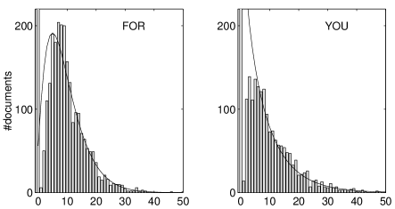
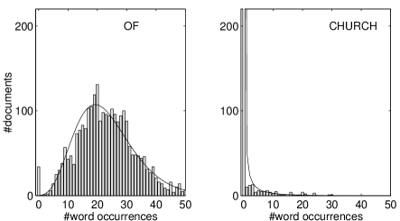
Figure 1: The occurrence of words (unigrams) varies between documents. Histograms show the number of word occurrences for ‘FOR’, ‘YOU’, ‘OF’, and ‘CHURCH’ from a set of 2583 documents, each containing at least 100 words (average: 497 words). A negative binomial distribution (solid line) was used to approximate each histogram. The number of word occurrences were normalised to 1000-word length documents.

Suppose the parameter $\lambda$ of the pdf (1) is distributed according to some function $\phi(\lambda)$, then we define a continuous mixture of Poisson distributions by

$$\theta(x)=\int_{0}^{\infty}\theta^{[p]}(x)\phi(\lambda)d\lambda\ .$$ (2)

In particular, if $\phi(\lambda)$ is a gamma distribution, i.e.,

$$\phi(\lambda)={\cal G}(\lambda;\ \alpha,\beta)=\frac{\lambda^{\alpha-1}e^{-\frac{\lambda}{\beta}}}{\beta^{\alpha}\Gamma(\alpha)}$$ (3)

for $\alpha>0$ and $\beta>0$, then the integral (2) is reduced to a discrete distribution for $x=0,1,\cdots$ such that

$$\theta^{[nb]}(x) = {\cal NB}(X=x;\ \alpha,\beta)$$ (6)

$$= \left(\begin{array}[]{c}\alpha+x-1\\ x\end{array}\right)\frac{\beta^{x}}{(1+\beta)^{\alpha+x}}\ .$$

This $\theta^{[nb]}(x)$ is a negative binomial distribution and its expectation and variance are respectively given by $E[X]=\alpha\beta$ and $V[X]=\alpha\beta(\beta+1)$.

2.3 Word Occurrences in Documents

The histograms in figure 1 show the number of word (unigram) occurrences in spoken news broadcast, taken from transcripts of the Hub–4E Broadcast News acoustic training data (1996–97). These transcripts were separated into documents according to section markers and those with less than 100 words were removed, resulting 2583 documents containing slightly less than 1.3 million words in total. In the following, the number of word occurrences were normalised to 1000-word length documents.

‘FOR’ and ‘YOU’ appeared approximately the same number of times across all the transcripts. Using a constant word rate assumption, they would have been assigned a probability of around 0.0086. However their occurrence rates varied from document to document; about 11% and 33% of all documents did not contain ‘FOR’ and ‘YOU’ (respectively), while 1% and 3% contained these words more than 30 times. This seems to indicate that occurrences of ‘FOR’ is less dependent on the content of the document. A negative binomial distribution was used to model the variable word rate in each case (the solid line in figure 1).

The negative binomial seems to model word occurrence rate relatively well for most vocabulary items, regardless of frequency. Figure 1 illustrates this for one of the most frequent words ‘OF’ (probability of 0.023 according to the constant word rate assumption) and the less frequently occurring ‘CHURCH’ (less than 0.00029). In particular, ‘CHURCH’ appeared only in 93 out of 2583 documents, but 28 of them contained more than 10 instances, suggesting strong correlation with document content.

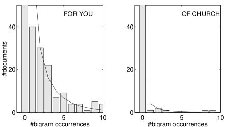
Figure 2: Variable bigram occurrence rates. Histograms show the number of bigram occurrences (in normalised 1000-word documents) for ‘FOR YOU’ and ‘OF CHURCH’, combinations of unigrams used in figure 1. They are fitted by negative binomial distributions (solid lines).

We also collected statistics of bigrams appearing in the Broadcast News transcripts. Figure 2 show histograms and their negative binomial fits for bigrams ‘FOR YOU’ and ‘OF CHURCH’. Although very sparse (e.g., they appeared in 127 and 6 documents, respectively), this suggests that variable bigram rate can also be modelled using a continuous mixture of Poissons.

3 Variable Word Rate Language Models

Taking word occurrence rate into account changes a probabilistic language model from a situation akin to playing a lottery, to something closer to betting on a horse race: the odds for a certain word improve if it has come up in the past. In this section, we eliminate the constant word rate assumption and present a variable word rate $n$-gram language model.

3.1 Relative Frequencies with Prior Word Occurrences

Let $f(w\geq n_{w})$ denote a relative frequency after we observe $n_{w}$ occurrences of word $w$. It is calculated by

$$f(w\geq n_{w})=\frac{1}{N}\frac{\displaystyle m_{w}-\sum_{j=0}^{n_{w}-1}j\cdot\theta_{w}(j)}{\displaystyle 1-\sum_{j=0}^{n_{w}-1}\theta_{w}(j)}\ .$$ (7)

The function is defined for $n_{w}=0,1,\cdots,N$, where $N$ is a fixed document length (e.g., $N$ is normalised to 1000 in figures 1 and 2). $\theta_{w}(j)$ is the occurrence rate for word $w$ in an $N$-length document (e.g., Poisson, negative binomial), satisfying

$$\sum_{j=0}^{N}j\cdot\theta_{w}(j)=m_{w}\ ,\hskip 14.45377pt\displaystyle\sum_{j=0}^{N}\theta_{w}(j)=1\ .$$

In particular,

$$\displaystyle f(w\geq 0)=\frac{m_{w}}{N}\ ,$$ (8)

which corresponds to the case with no prior information of word occurrence. For the conventional approach with the constant word rate assumption, this $f(w\geq 0)$ is not modified regardless of any word occurrences. Further, function (7) satisfies our intuition; the value of $f(w\geq n_{w})$ increases monotonically as the number of observation $n_{w}$ accumulates (easy to verify), and it reaches a unity (‘1’) when $n_{w}=N$.

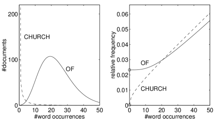
Figure 3: The left figure shows word occurrence rates for ‘OF’ and ‘CHURCH’ in documents of (normalised to) 1000-word length, modelled by negative binomial distributions (identical to those in figure 1). The right figure demonstrates relative frequencies after a certain number of word occurrences. Circles (‘o’) correspond to relative frequencies under the constant word rate assumption (0.023 for ‘OF’ and 0.00029 for ‘CHURCH’).

The characteristics of function (7) are illustrated in figure 3. The right hand figure shows relative frequencies for ‘OF’ and ‘CHURCH’ after a certain number of previous observations of the word. It indicates that the first few instances of the frequent word (‘OF’) do not modify its relative frequency very much, but have a substantial effect on the relative frequency of the less common word (‘CHURCH’). As the number of observations increases, the former is caught up by the latter.

Finally, in order to convert this relative frequency model to any type of probabilistic model for language, normalisation is required. This is achieved by dividing $f(w\geq n_{w})$ by $\displaystyle\sum_{w\in{\cal V}}f(w\geq n_{w})$, where ${\cal V}$ implies a set of vocabulary. Variable relative frequencies for bigrams can also be calculated in a similar fashion.

3.2 Discounting and Smoothing Techniques

For any practical application, smoothing of the probability estimates is essential to avoid zero probabilities for events that were not observed in the training data. Let ${\cal E}(w|v)$ denote a bigram entry (a word $v$ followed by $w$) in the model. Further, $f(w|v\geq n_{w|v})$ implies a relative frequency after we observe $n_{w|v}$ occurrences of the bigram. A bigram probability $p(w|v\geq n_{w|v})$ may be smoothed with a unigram probability $p(w\geq n_{w})$. Using the interpolation method [12]:

$$p(w|v\geq n_{w|v}) = \hat{f}(w|v\geq n_{w|v})$$ (9)

$$+\ \{1-\alpha(v)\}\cdot p(w\geq n_{w})$$

where $\hat{f}(w|v\geq n_{w|v})$ implies a “discounted” relative frequency (described later) and

$$\alpha(v)=\sum_{w\in{\cal E}(w|v)}\hat{f}(w|v\geq n_{w|v})$$ (10)

is a non-zero probability estimate (i.e., the probability that a bigram entry ${\cal E}(w|v)$ exists in the model). Alternatively, the back-off smoothing [13] may be applied:

$$p(w|v\geq n_{w|v})=\left\{\begin{array}[]{l}\hat{f}(w|v\geq n_{w|v})\hskip 11.38109pt\mbox{if }{\cal E}(w|v)\mbox{ exists},\\ \beta(v)\cdot p(w\geq n_{w})\hskip 11.38109pt\mbox{otherwise}.\end{array}\right.$$ (13)

In (13), $\beta(v)$ is a back-off factor and is calculated by

$$\beta(v)=\displaystyle\frac{1-\alpha(v)}{\displaystyle 1-\sum_{w\in{\cal E}(w|v)}\hat{f}(w\geq n_{w})}\ .$$ (14)

A unigram probability $p(w\geq n_{w})$ can be obtained similarly by smoothing with some constant value.

Finally, a number of standard discounting methods exist for constant word rate models (see, e.g., [13, 14]). Analogous discounting functions for variable word rate models may be

$$\hat{f}_{abs}(w|v\geq n_{w|v})=f(w|v\geq n_{w|v})-\frac{c}{N}$$ (15)

for the absolute discounting, and

$$\hat{f}_{gt}(w|v\geq n_{w|v})=d\cdot f(w|v\geq n_{w|v})$$ (16)

for the Good-Turing discounting. Discounting factors ($c$ and $d$) may be obtained using zero prior information case — i.e., $f(w|v\geq 0)$’s of all bigrams in the model — and the rest should be referred to, e.g., [13] or [14].

3.3 Language Model Perplexities

As noted in section 2, we extracted 2583 documents from the transcripts of the Broadcast News acoustic training data, each with a minimum of 100 words. A vocabulary of 19 885 words was selected and 390 000 bigrams were counted. In these experiments, the absolute discounting scheme (15) was applied, followed by interpolation smoothing (9). Figure 4 shows perplexities for the reference (key) transcription of the 1997 Hub–4E evaluation data, containing three hours of speech and approximately 32 000 words. Using conventional modelling with a constant word rate assumption, unigram and bigram perplexities were 936.5 and 237.9, respectively.

Figure 4: Unigram and bigram perplexities for the reference (key) transcription of 1997 Hub–4E evaluation data. Conventional models (constant word rate) are compared with models using Poisson estimates of variable word rate. Document length for the latter was normalised to between 200 and 50 000.

For the variable word rate models, the Poisson distribution was adopted because of simplicity in calculation. The number of word occurrences were normalised to $N$-word length document with $N$ being between 200 and 50 000, and the model parameters were modified ‘on-line’ during the perplexity calculation. For each occurrence of a word (bigram) in the evaluation data, a histogram of the past $N$ words (bigrams) was collected and their relative frequencies were modified according to the Poisson estimates (appropriate normalisation applied), then discounted and smoothed.

As figure 4 indicates, the variable word rate models were able to reduced perplexities from the constant word rate models. A unigram perplexity of 843.4 (10% reduction) was achieved when $N=500$, and a bigram perplexity of 219.0 (8% reduction) when $N=50\,000$. The difference was predictable because bigrams were orders of magnitude more sparse than unigrams.

4 Conclusion

In this paper, we have presented a variable word/$n$-gram rate language model, based upon an approach to estimating relative frequencies using prior information of word occurrences. Poisson and negative binomial models were used to approximate word occurrences in documents of fixed length. Using the Broadcast News task, the approach demonstrated a reduction of perplexity up to 10%, indicating potential although the technique is still premature. Because of the data sparsity problem, it is not clear if the approach can be applied to language model components of current state-of-the-art speech recognition systems that typically use 3/4-grams. However, we believe this technique does have application to problems in the area of information extraction. In particular, we are planning to apply these methods to the named entity annotation task, along with further theoretical development.

References

- [1] K. Spärck Jones, S. Walker, and S. E. Robertson. A probabilistic model of information retrieval: Development and status. Technical Report TR446, University of Cambridge, Computer Laboratory, 1998. Available from http://www.ftp.cl.cam.ac.uk/ftp/papers/reports/.
- [2] Abraham Bookstein and Don R. Swanson. Probabilistic models for automatic indexing. Journal of the American Society for Information Sceince, 25(5):312–318, September 1974.
- [3] Stephen P. Harter. A probabilistic approach to automatic keyword indexing (part i). Journal of the American Society for Information Sceince, 26(4):197–206, July 1975.
- [4] S. E. Robertson and S. Walker. Some simple effective approximations to the 2-Poisson model for probabilistic weighted retrieval. In Proceedings of SIGIR’94, pages 232–241, 1994.
- [5] Kenneth W. Church and William A. Gale. Poisson mixtures. Natural Language Engineering, 1(2):163–190, June 1995.
- [6] Stephen A. Lowe. The beta-binomial mixture model for word frequencies in documents with applications to information retrieval. In Proceedings of Eurospeech-99, volume 6, pages 2443–2446, Budapest, September 1999.
- [7] Reinhard Kneser and Volker Steinbiss. On the dynamic adaptation of stochastic language models. In Proceedings of ICASSP-93, volume II, pages 586–589, Minneapolis, April 1993.
- [8] Ronald Rosenfeld. A maximum entropy approach to adaptive statistical language modeling. Computer Speech and Language, 10:187–228, 1996.
- [9] R. Kuhn and R. De Mori. A cache-based natural language model for speech recognition. IEEE Transactions on Pattern Analysis and Machine Intelligence, 12(6):570–583, June 1990.
- [10] Samuel Karlin and Howard M. Taylor. A First Course in Stochastic Processes. Academic Press, 2nd edition, 1975.
- [11] Morris H. DeGroot. Optimal Statistical Decisions. McGraw Hill, New York, NY, 1970.
- [12] F. Jelinek and R. L. Mercer. Interpolated estimation of Markov source parameters from sparse data. In Proceedings of the Workshop: Pattern Recognition in Practice, pages 381–397, Amsterdam, May 1980.
- [13] Slava M. Katz. Estimation of probabilities from sparse data for the language model component of a speech recognizer. IEEE Transactions on Acoustics, Speech, and Signal Processing, 35(3):400–401, March 1987.
- [14] Hermann Ney, Ute Essen, and Reinhard Kneser. On the estimation of ‘small’ probabilities by leaving-one-out. IEEE Transactions on Pattern Analysis and Machine Intelligence, 17(12):1202–1212, December 1995.