Differential Invariants under Gamma Correction

Abstract

This paper presents invariants under gamma correction and similarity transformations. The invariants are local features based on differentials which are implemented using derivatives of the Gaussian. The use of the proposed invariant representation is shown to yield improved correlation results in a template matching scenario.

1 Introduction

Invariants are a popular concept in object recognition and image retrieval [1, 2, 7, 10, 14, 15]. They aim to provide descriptions that remain constant under certain geometric or radiometric transformations of the scene, thereby reducing the search space. They can be classified into global invariants, typically based either on a set of key points or on moments, and local invariants, typically based on derivatives of the image function which is assumed to be continuous and differentiable.

The geometric transformations of interest often include translation, rotation, and scaling, summarily referred to as similarity transformations. In a previous paper [12], building on work done by Schmid and Mohr [11], we have proposed differential invariants for those similarity transformations, plus linear brightness change. Here, we are looking at a non-linear brightness change known as gamma correction.

Gamma correction is a non-linear quantization of the brightness measurements performed by many cameras during the image formation process. The idea is to achieve better perceptual results by maintaining an approximately constant ratio between adjacent brightness levels, placing the quantization levels apart by the just noticeable difference. Incidentally, this non-linear quantization also precompensates for the non-linear mapping from voltage to brightness in electronic display devices [4, 9].

Gamma correction can be expressed by the equation

$$I_{\gamma}=p\,I^{\gamma}$$ (1)

where $I$ is the input intensity, $I_{\gamma}$ is the output intensity, and $p$ is a normalization factor which is determined by the value of $\gamma$. For output devices, the NTSC standard specifies $\gamma=2.22$. For input devices like cameras, the parameter value is just inversed, resulting in a typical value of $\gamma=1/2.22=0.45$. The camera we used, the Sony 3 CCD color camera DXC 950, exhibited $\gamma\approx 0.6$. Fig. 1 shows the intensity mapping of 8-bit data for different values of $\gamma$.

Figure 1: Gamma correction as a function of intensity.  (solid)  $\gamma=1$;  (dashed) $\gamma=0.45$;  (dotted) $\gamma=2.22$. Note how, for $\gamma<1$, the lower intensities are mapped onto a larger range.

It turns out that an invariant under gamma correction can be designed from first and second order derivatives. Additional invariance under scaling requires third order derivatives. Derivatives are by nature translationally invariant. Rotational invariance in 2-d is achieved by using rotationally symmetric operators.

2 The Invariants

The key idea for the design of the proposed invariants is to form suitable ratios of the derivatives of the image function such that the parameters describing the transformation of interest will cancel out. This idea has been used in [12] to achieve invariance under linear brightness changes, and it can be adjusted to the context of gamma correction by – at least conceptually – considering the logarithm of the image function. For simplicity, we begin with 1-d image functions.

2.1 Invariance under Gamma Correction

Let $f(x)$ be the image function, i.e. the original signal, assumed to be continuous and differentiable, and $f_{\gamma}(x)=p\,f(x)^{\gamma}$ the corresponding gamma corrected function. Note that $f(x)$ is a special case of $f_{\gamma}(x)$ where $\gamma=p=1$. Taking the logarithm yields

$$\tilde{f}_{\gamma}(x)=\ln(p\,f(x)^{\gamma})=\ln p+\gamma\ln f(x)$$ (2)

with the derivatives $\tilde{f}^{\prime}_{\gamma}(x)=\gamma\,f^{\prime}(x)/f(x)$, and $\tilde{f}^{\prime\prime}_{\gamma}(x)=\gamma\,(f(x)\,f^{\prime\prime}(x)-f^{\prime}(x)^{2})/f(x)^{2}$. We can now define the invariant $\Theta_{12\gamma}$ under gamma correction to be

$$\Theta_{12\gamma}(f(x))$$ =

=

=

(3)

The factor $p$ has been eliminated by taking derivatives, and $\gamma$ has canceled out. Furthermore, $\Theta_{12\gamma}$ turns out to be completely specified in terms of the original image function and its derivatives, i.e. the logarithm actually doesn’t have to be computed. The notation $\Theta_{12\gamma}(f(x))$ indicates that the invariant depends on the underlying image function $f(x)$ and location $x$ – the invariance holds under gamma correction, not under spatial changes of the image function.

A shortcoming of $\Theta_{12\gamma}$ is that it is undefined where the denominator is zero. Therefore, we modify $\Theta_{12\gamma}$ to be continuous everywhere:

0 if $$f\,f^{\prime}=0\wedge f\,f^{\prime\prime}-{f^{\prime}}^{2}=0$$

if

else

(4)

where, for notational convenience, we have dropped the variable $x$. The modification entails $-1\leq\Theta_{m12\gamma}\leq 1$. Note that the modification is just a heuristic to deal with poles. If all derivatives are zero because the image function is constant, then differentials are certainly not the best way to represent the function.

2.2 Invariance under Gamma Correction and Scaling

If scaling is a transformation that has to be considered, then another parameter $\alpha$ describing the change of size has to be introduced. That is, scaling is modeled here as variable substitution [11]: the scaled version of $f(x)$ is $g(\alpha x)=g(u)$. So we are looking at the function

$$\tilde{f}_{\gamma}(x)=\ln(pf(x)^{\gamma})=\ln p+\gamma\ln g(\alpha x)=\tilde{g}_{\gamma}(u)$$

where the derivatives with respect to $x$ are $\tilde{g}^{\prime}_{\gamma}(u)=\gamma\alpha\,g^{\prime}(u)/g(u)$, $\tilde{g}^{\prime\prime}_{\gamma}(u)=\gamma\alpha^{2}(g(u)\,g^{\prime\prime}(u)-g^{\prime}(u)^{2})/g(u)^{2}$, and $\tilde{g}^{\prime\prime\prime}_{\gamma}(u)=\gamma\alpha^{3}\,\bigl{(}g^{\prime\prime\prime}(u)/g(u)-3\,g^{\prime}(u)\,g^{\prime\prime}(u)/g(u)^{2}+2\,g^{\prime}(u)^{3}/g(u)^{3}\bigr{)}$. Now the invariant $\Theta_{123\gamma}(g(u))$ is obtained by defining a suitable ratio of the derivatives such that both $\gamma$ and $\alpha$ cancel out:

$$\Theta_{123\gamma}(g(u))$$ =

=

(5)

Analogously to eq. (4), we can define a modified invariant

0 if cond1

$$\Theta_{m123\gamma}=$$ if cond2

else

(6)

where condition cond1 is $g^{2}g^{\prime}\,g^{\prime\prime\prime}-3\,g\,{g^{\prime}}^{2}g^{\prime\prime}+2\,{g^{\prime}}^{4}=0$ $\wedge$ $g^{2}{g^{\prime\prime}}^{2}-2\,g\,{g^{\prime}}^{2}g^{\prime\prime}+\ {g^{\prime}}^{4}=0$, and condition cond2 is $|{g^{2}g^{\prime}\,g^{\prime\prime\prime}-3\,g\,{g^{\prime}}^{2}g^{\prime\prime}+2\,{g^{\prime}}^{4}}|$ $<$ $|{g^{2}{g^{\prime\prime}}^{2}-2\,g\,{g^{\prime}}^{2}g^{\prime\prime}+\ {g^{\prime}}^{4}}|$. Again, this modification entails $-1\leq\Theta_{m123\gamma}\leq 1$.

2.3 An Analytical Example

It is a straightforward albeit cumbersome exercise to verify the invariants from eqs. (3) and (5) with an analytical, differentiable function. As an arbitrary example, we choose

$$f(x)=3x\sin(2\pi x)+30$$

The first three derivatives are $f^{\prime}(x)=3\sin(2\pi x)+6\pi x\cos(2\pi x)$, $f^{\prime\prime}(x)=12\pi\cos(2\pi x)-12\pi^{2}x\sin(2\pi x)$, and $f^{\prime\prime\prime}(x)=-36\pi^{2}\sin(2\pi x)-24\pi^{3}x\cos(2\pi x)$. Then, according to eq. (3), $\Theta_{12\gamma}(f(x))=(3x\sin(2\pi x)+30)\,(3x\sin(2\pi x)+6\pi x\cos(2\pi x))\,/\,\bigl{(}(3x\sin(2\pi x)+30)\,(12\pi\cos(2\pi x)-12\pi^{2}x\sin(2\pi x))-(3\sin(2\pi x)+6\pi x\cos(2\pi x))^{2}\bigr{)}$.

If we now replace $f(x)$ with a gamma corrected version, say $f_{0.45}(x)=255^{1-0.45}\cdot 3x\sin(2\pi x)+30)^{0.45}$, the first derivative becomes $f^{\prime}_{0.45}(x)=255^{0.55}\cdot 0.45\,(3\sin(2\pi x)+30)^{-0.55}(3\sin(2\pi x)+6\pi x\cos(2\pi x))$, the second derivative is $f^{\prime\prime}_{0.45}(x)=-255^{0.55}\cdot 0.45\cdot 0.55\,(3\sin(2\pi x)+30)^{-1.55}(3\sin(2\pi x)+6\pi x\cos(2\pi x))^{2}+255^{0.55}\cdot 0.45\,(3x\sin(2\pi x)+30)^{-0.55}(12\pi\cos(2\pi x)-12\pi^{2}x\sin(2\pi x))$, and the third is $f^{\prime\prime\prime}_{0.45}(x)=255^{0.55}\cdot 0.45\,(3\sin(2\pi x)+30)^{-0.55}\bigl{(}1.55\cdot 0.55\,(3\sin(2\pi x)+30)^{-2}(3\sin(2\pi x)+6\pi x\cos(2\pi x))^{3}+\ (-3)\cdot 0.55\,(3\sin(2\pi x)+30)^{-1}(3\sin(2\pi x)+6\pi x\cos(2\pi x))\,(12\pi\cos(2\pi x)-12\pi^{2}x\sin(2\pi x))+(-36\pi^{2}\sin(2\pi x)-24\pi^{3}x\cos(2\pi x))\bigr{)}$. If we plug these derivatives into eq. (3), we obtain an expression for $\Theta_{12\gamma}(f_{0.45}(x))$ which is identical to the one for $\Theta_{12\gamma}(f(x))$ above. The algebraically inclined reader is encouraged to verify the invariant $\Theta_{123\gamma}$ for the same function.

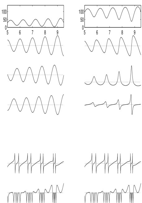
Figure 2: An analytical example function.  (left) $f(x)=3x\sin(2\pi x)+30$;  (right) $f_{\gamma}(x)=p\,f(x)^{\gamma}$, $\gamma=0.45$.  (first row) original functions  (second row) first derivatives;  (third row) second derivatives;  (fourth row) third derivatives;  (fifth row) $\Theta_{m12\gamma}$;  (sixth row) $\Theta_{m123\gamma}$.

Fig. 2 shows the example function and its gamma corrected counterpart, together with their derivatives and the two modified invariants. As expected, the graphs of the invariants are the same on the right as on the left. Note that the invariants define a many-to-one mapping. That is, the mapping is not information preserving, and it is not possible to reconstruct the original image from its invariant representation.

2.4 Extension to 2-d

If $\Theta_{m12\gamma}$ or $\Theta_{m123\gamma}$ are to be computed on images, then eqs. (3) to (6) have to be generalized to two dimensions. This is to be done in a rotationally invariant way in order to achieve invariance under similarity transformations. The standard way is to use rotationally symmetric operators. For the first derivative, we have the well known gradient magnitude, defined as

$$\nabla(x,y)=\sqrt{I_{x}^{2}+I_{y}^{2}}:=I^{\prime}$$ (7)

where $I(x,y)$ is the 2-d image function, and $I_{x}$, $I_{y}$ are partial derivatives along the x-axis and the y-axis. For the second order derivative, we can use the linear Laplacian

$$\nabla^{2}(x,y)=I_{xx}+I_{yy}:=I^{\prime\prime}$$ (8)

Horn [5] also presents an alternative second order derivative operator, the quadratic variation

$$\mathrm{QV}(x,y)=\sqrt{I_{xx}^{2}+2I_{xy}^{2}+I_{yy}^{2}}$$ (9)

Since the QV is not a linear operator and more expensive to compute, we use the Laplacian for our implementation. For the third order derivative, we can define, in close analogy with the quadratic variation, a cubic variation as

$$\mathrm{CV}(x,y)=\sqrt{I_{xxx}^{2}+3I_{xxy}^{2}+3I_{xyy}^{2}+I_{yyy}^{2}}:=I^{\prime\prime\prime}$$ (10)

The invariants from eqs. (3) to (6) remain valid in 2-d if we replace $f^{\prime}$ with $I^{\prime}$, $f^{\prime\prime}$ with $I^{\prime\prime}$, and $f^{\prime\prime\prime}$ with $I^{\prime\prime\prime}$. This can be verified by going through the same argument as for the 1-d functions. Recall that the critical observation in eq. (3) was that $\gamma$ cancels out, which is the case when all derivatives return a factor $\gamma$. But such is also the case with the rotationally symmetric operators mentioned above. For example, if we apply the gradient magnitude operator to $\tilde{I}(x,y)$, i.e. to the logarithm of a gamma corrected image function, we obtain

$$\nabla=\sqrt{\tilde{I}_{x}^{2}+\tilde{I}_{y}^{2}}=\sqrt{\bigl{(}\gamma\,\frac{I_{x}}{I}\bigr{)}^{2}+\bigl{(}\gamma\,\frac{I_{y}}{I}\bigr{)}^{2}}=\gamma\,\frac{\sqrt{I_{x}^{2}+I_{y}^{2}}}{I}$$

returning a factor $\gamma$, and analogously for $\nabla^{2}$, QV, and CV. A similar argument holds for eq. (5) where we have to show, in addition, that the first derivative returns a factor $\alpha$, the second derivative returns a factor $\alpha^{2}$, and the third derivative returns a factor $\alpha^{3}$, which is the case for our 2-d operators.

2.5 Differential Operators

While the derivatives of continuous, differentiable functions are uniquely defined, there are many ways to implement derivatives for sampled functions. We follow Schmid and Mohr [11], ter Haar Romeny [13], and many other researchers in employing the derivatives of the Gaussian function as filters to compute the derivatives of a sampled image function via convolution. This way, derivation is combined with smoothing. The 2-d zero mean Gaussian is defined as

$$G=\frac{1}{2\pi\,\sigma^{2}}\ e^{-\frac{x^{2}+y^{2}}{2\sigma^{2}}}$$ (11)

The partial derivatives up to third order are $G_{x}=-x/\sigma^{2}\,G$, $G_{y}=-y/\sigma^{2}\,G$, $G_{xx}=(x^{2}-\sigma^{2})/\sigma^{4}\,G$, $G_{xy}=xy/\sigma^{4}\,G$, $G_{yy}=(y^{2}-\sigma^{2})/\sigma^{4}\,G$, $G_{xxx}=(3\sigma^{2}x-x^{3})/\sigma^{6}\,G$, $G_{xxy}=(\sigma^{2}y-x^{2}y)/\sigma^{6}\,G$, $G_{xyy}=(\sigma^{2}x-xy^{2})/\sigma^{6}\,G$, $G_{yyy}=(3\sigma^{2}y-y^{3})/\sigma^{6}\,G$. They are shown in fig. 3. We used the parameter setting $\sigma=1.0$ and kernel size $7\times 7$. With these kernels, eq. (3), for example, is implemented as

$$\Theta_{12\gamma}=\frac{I\,\sqrt{(I\circledast G_{x})^{2}+(I\circledast G_{y})^{2}}}{I\,(I\circledast G_{xx}+I\circledast G_{yy})\,-\,((I\circledast G_{x})^{2}+(I\circledast G_{y})^{2})}$$

at each pixel $(x,y)$, where $\circledast$ denotes convolution.

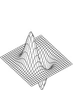
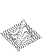
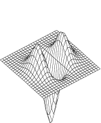
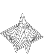
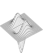
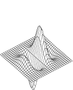
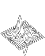
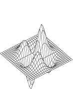
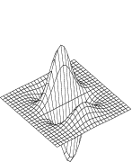
Figure 3: Partial derivatives of the 2-d Gaussian.  (first row) $G_{x}$, $G_{y}$, $G_{xx}$;  (second row) $G_{xy}$, $G_{yy}$, $G_{xxx}$;  (third row) $G_{xxy}$, $G_{xyy}$, $G_{yyy}$.

3 Experimental Data and Results

We evaluate the invariant $\Theta_{m12\gamma}$ from eq. (4) in two different ways. First, we measure how much the invariant computed on an image without gamma correction is different from the invariant computed on the same image but with gamma correction. Theoretical, this difference should be zero, but in practice, it is not. Second, we compare template matching accuracy on intensity images, again without and with gamma correction, to the accuracy achievable if instead the invariant representation is used. We also examine whether the results can be improved by prefiltering.

3.1 Absolute and Relative Errors

A straightforward error measure is the absolute error,

$$\Delta_{GC}(i,j)=|\Theta_{GC}(i,j)-\Theta_{0GC}(i,j)|$$ (12)

where ”0GC” refers to the image without gamma correction, and GC stands for either ”SGC” if the gamma correction is done synthetically via eq. (1), or for ”CGC” if the gamma correction is done via the camera hardware. Like the invariant itself, the absolute error is computed at each pixel location $(i,j)$ of the image, except for the image boundaries where the derivatives and therefore the invariants cannot be computed reliably.

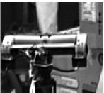
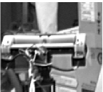
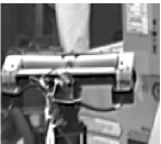
Figure 4: Example image WoBA:  (a) no gamma correction, “0GC”;  (b) gamma correction by camera, “CGC”;  (c) synthetic gamma correction, “SGC”.

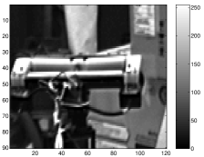
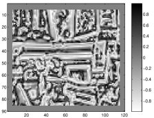
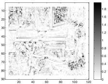
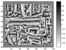
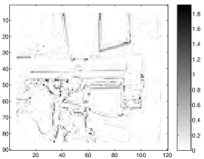
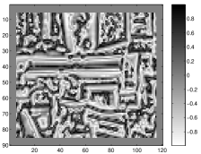
Figure 5: Absolute errors for invariant $\Theta_{m12\gamma}$, no prefiltering. (a) image WoBA, 0GC; (b) $\Theta_{0GC}$; (c) $\Delta_{CGC}$; (d) $\Theta_{CGC}$; (e) $\Delta_{SGC}$; (f) $\Theta_{SGC}$.

Fig. 4 shows an example image. The SGC image has been computed from the 0GC image, with $\gamma=0.6$. Note that the gamma correction is done after the quantization of the 0GC image, since we don’t have access to the 0GC image before quantization.

Fig. 5 shows the invariant representations of the image data from fig. 4 and the corresponding absolute errors. Since $-1\leq\Theta_{m12\gamma}\leq 1$, we have $0\leq\Delta_{GC}\leq 2$. The dark points in fig. 5, (c) and (e), indicate areas of large errors. We observe two error sources:

• The invariant cannot be computed robustly in homogeneous regions. This is hardly surprising, given that it is based on differentials which are by definition only sensitive to spatial changes of the signal.

• There are outliers even in the SGC invariant representation, at points of very high contrast edges. They are a byproduct of the inherent smoothing when the derivatives are computed with differentials of the Gaussian. Note that the latter put a ceiling on the maximum gradient magnitude that is computable on 8-bit images.

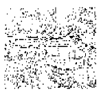
Figure 6: Reliable points $\mathrm{RP}_{\epsilon}$ for invariant $\Theta_{m12\gamma}$, in black, image WoBA, without and with prefiltering.  (a) $\sigma_{pre}$=0,  $\epsilon$= 5.0;  (b) $\sigma_{pre}$=0,  $\epsilon$=10.0;  (c) $\sigma_{pre}$=0,  $\epsilon$=20.0;  (d) $\sigma_{pre}$=1.0, $\epsilon$= 5.0;  (e) $\sigma_{pre}$=1.0, $\epsilon$=10.0;  (f) $\sigma_{pre}$=1.0, $\epsilon$=20.0.

In addition to computing the absolute error, we can also compute the relative error, in percent, as

$$\delta_{CGC}(i,j)=100\ \Delta_{CGC}(i,j)\,/\,\Theta_{0GC}(i,j)$$ (13)

Then we can define the set $\mathrm{RP}_{\epsilon}$ of reliable points, relative to some error threshold $\epsilon$, as

$$\mathrm{RP}_{\epsilon}=\{(i,j)\,|\,\delta(i,j)\leq\epsilon\}$$ (14)

and $\mathrm{PRP}_{\epsilon}$, the percentage of reliable points, as

$$\mathrm{PRP}_{\epsilon}=100\ |\mathrm{RP}_{\epsilon}|\,/\,n$$ (15)

where $n$ is the number of valid, i.e. non-boundary, pixels in the image. Fig. 6 shows, in the first row, the reliable points for three different values of the threshold $\epsilon$. The second row shows the sets of reliable points for the same thresholds if we gently prefilter the 0GC and CGC images. The corresponding data for the ten test images from fig. 11 is summarized in table 1.

image	5.0	10.0	20.0	5.0	10.0	20.0
Build	13.3	24.9	43.8	16.0	29.5	49.3
WoBA	15.6	29.0	48.2	19.0	35.7	58.9
WoBB	16.5	28.7	47.1	21.4	37.7	58.1
WoBC	18.5	33.6	53.5	24.0	41.4	65.3
WoBD	13.0	23.9	41.9	16.7	32.6	55.6
Cycl	15.4	28.3	45.9	22.6	38.8	57.6
Sand	14.5	27.2	44.7	22.0	38.5	57.6
ToolA	5.6	10.7	20.1	7.4	14.7	27.1
ToolB	6.1	12.0	22.7	8.3	15.7	28.6
ToolC	5.6	11.1	20.8	7.9	15.1	28.3
median	13.9	26.1	44.3	17.9	34.2	56.6
mean	12.4	22.9	38.9	16.5	30.0	48.6

Table 1: Percentages of reliable points for $\Theta_{m12\gamma}$, CGC images, for $\epsilon$=5.0, 10.0, 20.0. The three numerical columns on the left show $\mathrm{PRP}_{\epsilon}$ without prefiltering, the three right columns with Gaussian prefiltering, $\sigma_{pre}$=1.0.

Derivatives are known to be sensitive to noise. Noise can be reduced by smoothing the original data before the invariants are computed. On the other hand, derivatives should be computed as locally as possible. With these conflicting goals to be considered, we experiment with gentle prefiltering, using a Gaussian filter of size $\sigma_{pre}$=1.0. The size of the Gaussian to compute the invariant $\Theta_{m12\gamma}$ is set to $\sigma_{der}$=1.0. Note that $\sigma_{pre}$ and $\sigma_{der}$ can not be combined into just one Gaussian because of the non-linearity of the invariant.

With respect to the set of reliable points, we observe that after prefiltering, roughly half the points, on average, have a relative error of less than 20%. Gentle prefiltering consistently reduces both absolute and relative errors, but strong prefiltering does not.

3.2 Template Matching

Template matching is a frequently employed technique in computer vision. Here, we will examine how gamma correction affects the spatial accuracy of template matching, and whether that accuracy can be improved by using the invariant $\Theta_{m12\gamma}$.

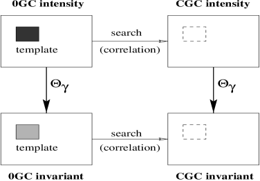
Figure 7: The template location problem: A query template is cut out from the 0GC intensity image and correlated with the corresponding CGC intensity image. We test if the correlation maximum occurs at exactly the same location as in the 0GC intensity image. The same process is repeated with the invariant representations of the 0GC and CGC images.

An overview of the testbed scenario is given in fig. 7. A small template of size $6\times 8$, representing the search pattern, is taken from a 0GC intensity image, i.e. without gamma correction. This query template is then correlated with the corresponding CGC intensity image, i.e. the same scene but with gamma correction switched on. If the correlation maximum occurs at exactly the location where the 0GC query template has been cut out, we call this a correct maximum correlation position, or CMCP.

The correlation function $s(x,y)$ employed here is based on a normalized mean squared difference $c(x,y)$ [3]:

$$s =\max(0,1-c)$$

$$c =\frac{\sum_{i,j}((I(x+i,y+j)-\overline{I})-(T(i,j)-\overline{T}))^{2}}{\sqrt{\sum_{i,j}(I(x+i,y+j)-\overline{I})^{2}\ \sum_{i,j}(T(i,j)-\overline{T})^{2}}}$$

where $I$ is an image, $T$ is a template positioned at $(x,y)$, $\overline{I}(x,y)$ is the mean of the subimage of $I$ at $(x,y)$ of the same size as $T$, $\overline{T}$ is the mean of the template, and $0\leq s\leq 1$. The template location problem then is to perform this correlation for the whole image and to determine whether the position of the correlation maximum occurs precisely at $(x,y)$.

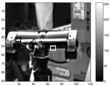
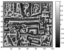
Figure 8: Matched templates, image WoBA:  (left) intensity data;  (right) invariant representation. Black box=query template, white box=matched template.

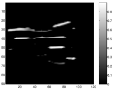
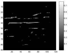
Figure 9: Correlation matrices, image WoBA.  (left) intensity data;  (right) invariant representation.

Fig. 8 demonstrates the template location problem, on the left for an intensity image, and on the right for its invariant representation. The black box marks the position of the original template at (40,15), and the white box marks the position of the matched template, which is incorrectly located at (50,64) in the intensity image. On the right, the matched template (white) has overwritten the original template (black) at the same, correctly identified position. Fig. 9 visualizes the correlation function over the whole image. The white areas are regions of high correlation.

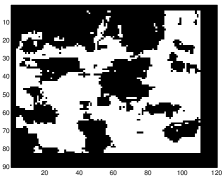
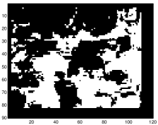
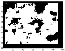
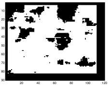
Figure 10: Binary correlation accuracy matrices, white pixels=$CMCP_{6\times 8}$, image WoBA.  (a) intensity image, $\sigma_{pre}$=0;  (b) intensity image, $\sigma_{pre}$=1.0;  (c) invariant representation, $\sigma_{pre}$=0;  (d) invariant representation, $\sigma_{pre}$=1.0.

The example from figs. 8 and 9 deals with only one arbitrarily selected template. In order to systematically analyze the template location problem, we repeat the correlation process for all possible template locations. Then we can define the correlation accuracy CA as the percentage of correctly located templates,

$$\mathrm{CA}_{tn\times tm}=100\ |\mathrm{CMCP}_{tn\times tm}|\,/\,n$$ (16)

where $tn\times tm$ is the size of the template, $\mathrm{CMCP}_{tn\times tm}$ is the set of correct maximum correlation positions, and $n$, again, is the number of valid pixels. We compute the correlation accuracy both for unfiltered images and for gently prefiltered images, with $\sigma_{pre}=1.0$. Fig. 10 shows the binary correlation accuracy matrices for our example image. The CMCP set is shown in white, its complement and the boundaries in black. We observe a higher correlation accuracy for the invariant representation, which is improved by the prefiltering.

Figure 11: Test images: (a) Build; (b) WoBA; (c) WoBB; (d) WoBC; (e) WoBD; (f) Cycl; (g) Sand; (h) ToolA; (i) ToolB; (j) ToolC.

image	Int/0	Int/1.0	Inv/0	Inv/1.0
Build	85.0	78.0	85.8	89.5
WoBA	55.5	45.0	75.7	80.4
WoBB	39.3	31.0	52.7	57.6
WoBC	67.2	58.3	68.9	78.7
WoBD	31.6	29.2	48.0	67.4
Cycl	60.5	45.4	98.6	99.4
Sand	50.5	40.9	85.2	94.4
ToolA	41.7	35.3	60.2	68.0
ToolB	29.5	23.4	45.7	54.1
ToolC	42.1	27.8	42.5	48.4
median	46.3	38.1	64.6	73.4
mean	50.3	41.4	66.3	73.8

Table 2: Correlation accuracies CA, template size $6\times 8$, left columns for intensity data, right columns for the invariant representation, without and with prefiltering.

Figure 12: Correlation accuracies,  (top) template size $6\times 8$;  (bottom) template size $10\times 10$. The entries at x=1 refer to Build, at x=2 to WoBA, etc.  (circles, lower line) intensity images;  (stars, center line) invariant representation, $\sigma_{pre}$=0;  (diamonds, upper line) invariant representation, $\sigma_{pre}$=1.0. The markers on the left hand side indicate the means, the markers on the right hand side the medians.

We have computed the correlation accuracy for all the images given in fig. 11. The results are shown in table 2 and visualized in fig. 12. We observe the following:

• The correlation accuracy CA is higher on the invariant representation than on the intensity images.

• The correlation accuracy is higher on the invariant representation with gentle prefiltering, $\sigma_{pre}=1.0$, than without prefiltering. We also observed a decrease in correlation accuracy if we increase the prefiltering well beyond $\sigma_{pre}=1.0$. By contrast, prefiltering seems to be always detrimental to the intensity images CA.

• The correlation accuracy shows a wide variation, roughly in the range 30%$\dots$90% for the unfiltered intensity images and 50%$\dots$100% for prefiltered invariant representations. Similarly, the gain in correlation accuracy ranges from close to zero up to 45%. For our test images, it turns out that the invariant representation is always superior, but that doesn’t necessarily have to be the case.

• The medians and means of the CAs over all test images confirm the gain in correlation accuracy for the invariant representation.

• The larger the template size, the higher the correlation accuracy, independent of the representation. A larger template size means more structure, and more discriminatory power.

4 Conclusion

We have proposed novel invariants that combine invariance under gamma correction with invariance under geometric transformations. In a general sense, the invariants can be seen as trading off derivatives for a power law parameter, which makes them interesting for applications beyond image processing. The error analysis of our implementation on real images has shown that, for sampled data, the invariants cannot be computed robustly everywhere. Nevertheless, the template matching application scenario has demonstrated that a performance gain is achievable by using the proposed invariant.

5 Acknowledgements

Bob Woodham suggested to the author to look into invariance under gamma correction. His meticulous comments on this work were much appreciated. Jochen Lang helped with the acquisition of image data through the ACME facility [8].

References

- [1] R. Alferez, Y. Wang, “Geometric and Illumination Invariants for Object Recognition”, IEEE Transactions on Pattern Analysis and Machine Intelligence, Vol.21, No.6, pp.505-537, June 1999.
- [2] D. Forsyth, J. Mundy, A. Zisserman, C. Coelho, C. Rothwell, “Invariant Descriptors for 3-D Object Recognition and Pose”, IEEE Transactions on Pattern Analysis and Machine Intelligence, Vol.13, No.10, pp.971-991, Oct.1991.
- [3] P. Fua, “A parallel stereo algorithm that produces dense depth maps and preserves image features”, Machine Vision and Applications, Vol.6, pp.35-49, 1993.
- [4] G. Holst, “CCD arrays, cameras, and displays”, JCD Publishing & SPIE Press, 2nd ed., 1998.
- [5] B. Horn, “Robot Vision”, MIT Press, 1986.
- [6] G. Martin, “High-Resolution Color CCD Camera”, Proc. SPIE Conference on Cameras, Scanners, and Image Acquisition Systems,pp.120-135, San Jose 1993.
- [7] J. Mundy, A. Zisserman, “Geometric Invariance in Computer Vision”, MIT Press, Cambridge 1992.
- [8] D. Pai, J. Lang, J. Lloyd, R. Woodham, “ACME, A Telerobotic Active Measurement Facility”, Sixth International Symposium on Experimental Robotics, Sydney, 1999. See also: http://www.cs.ubc.ca/nest/lci/acme/
- [9] C. Poynton, “A Technical Introduction to Digital Video”, John Wiley & Sons, 1996. See also http://www.inforamp.net/ poynton/GammaFAQ.html.
- [10] E. Rivlin, I. Weiss, “Local Invariants for Recognition”, IEEE Transactions on Pattern Analysis and Machine Intelligence, Vol.17, No.3, pp.226-238, Mar.1995.
- [11] C. Schmid, R. Mohr, “Local grayvalue invariants for Image Retrieval”, IEEE Transactions on Pattern Analysis and Machine Intelligence, Vol.19, No.5, pp.530-535, May 1997.
- [12] A. Siebert, “A Differential Invariant for Zooming”, ICIP-99, Kobe 1999.
- [13] B. ter Haar Romeny, “Geometry-Driven Diffusion in Computer Vision”, Kluwer 1994.
- [14] I. Weiss, “Geometric Invariants and Object Recognition”, International Journal of Computer Vision, Vol.10, No.3, pp.207-231, 1993.
- [15] J. Wood, “Invariant Pattern Recognition: A Review”, Pattern Recognition, Vol.29, No.1, pp.1-17, 1996.