Multiplicative Algorithm for Orthgonal Groups
and Independent Component Analysis

Abstract

The multiplicative Newton-like method developed by the author et al. is extended to the situation where the dynamics is restricted to the orthogonal group. A general framework is constructed without specifying the cost function. Though the restriction to the orthogonal groups makes the problem somewhat complicated, an explicit expression for the amount of individual jumps is obtained. This algorithm is exactly second-order-convergent. The global instability inherent in the Newton method is remedied by a Levenberg-Marquardt-type variation. The method thus constructed can readily be applied to the independent component analysis. Its remarkable performance is illustrated by a numerical simulation.

1 Overview

Many optimization problems take the form, “Find an optimal matrix under the constraints (1).. (2).. etc.” Some of these can be considered as optimizations on Lie groups. For groups, the fundamental manipulation is a multiplication whereas an addition is unnatural. In consideration of this fact, we have constructed a multiplicative Newton-like algorithm for maximizing the kurtosis (a good barometer for the independence) in [T.Akuzawa & N.Murata,1999]. There the dynamics takes place on the coset $GL(1,{\mathbb{R}})^{N}\backslash GL(N,{\mathbb{R}})$. We can apply the techniques developed in [T.Akuzawa & N.Murata,1999] to many other optimization problems. The coset structure $GL(1,{\mathbb{R}})^{N}\backslash GL(N,{\mathbb{R}})$ is, however, characteristic of the independent component analysis(ICA). It is understood by the fact that the independence is nothing to do with the scaling. The redundancy resulting from the invariance of the model under the componentwise scaling must be eliminated for a rigorous discussion and this redundancy corresponds to $GL(1,{\mathbb{R}})^{N}$.

Another way to eliminate this redundancy is the prewhitening. The prewhitening is a linear transformation of the observed data which maps the covariance matrix to the unit matrix. If we deal with prewhitened data, we can legitimately narrow the sweeping range to the orthogonal group. The aim of this letter is the construction of a multiplicative algorithm for the orthogonal groups.

The framework is as follows. $N$-dimensional prewhitened random variables $\{X_{i}|1\leq i\leq N\}$ are available and it is anticipated that their origins are some unknown mutually independent components $\{Y_{i}^{*}|1\leq i\leq N\}$. The goal of the ICA is the map $\{X_{i}\}\mapsto\{Y_{i}^{*}\}$. We restrict ourselves to the linear independent component analysis. There we want to find a linear transformation $C^{*}:{X}=(X_{1},\cdots,X_{N})^{\prime}\mapsto{Y^{*}}=(Y_{1}^{*},\cdots,Y_{N}^{*})^{\prime}=C^{*}{X}$ which minimizes some cost function that measures the independence. Since we are assuming that the data is already prewhitened, the covariance matrix of $X$ is the $N\times N$ unit matrix. If we do not take into account errors in the prewhitening, the optimal point $C^{*}$ must belong to $O(N)$.

Giving up the analytical solution, we consider a sequence,

$$C(0),~{}C{(1)},~{}C{(2)},~{}C{(3)},~{}\cdots\cdots~{},$$ (1.1)

which converges to the optimal solution $C^{*}$. The sequence $\{C(t)\}$ is generated by the left-multiplication of another sequence of orthogonal matrices $\{D(t)\}$. Each $D(t)$ is specified by the coordinate $\Delta(t)$ which satisfies $D(t)={\rm e}^{\Delta(t)}$. We assume that $\Delta(t)$ is an $N\times N$ skew-symmetric matrix, which implies that $D(t)$ belongs to the identity component of $O(N)$. In practice the procedure is as follows. As an initial condition we set $C(0)$. For $t>0~{}(t\in{\mathbb{N}}^{+})$, we introduce $\Delta(t)$ and denote $C({t})$ as $C({t+1})={\rm e}^{\Delta({t})}C(t)$. Under these settings, we determine $\Delta(t)$ by using the Newton method with respect to the matrix elements of $\Delta(t)$. That is, we evaluate the cost function at $C({t+1})$ by expanding it around $C({t})$ in terms of the elements of $\Delta({t})$ up to the second order. Then $\Delta(t)$ is choosen as the (unique) critical point of this second order expansion. We iteratively follow these procedures until we obtain a satisfactory solution.

This letter is organized as follows. In Section 2 we will give a complete description of a new multiplicative updating method for the orthogonal groups. This section is the main part of this letter. Since our formulation does not depend on the details of the cost function the method can be useful for many problems other than the ICA. The performance of our method including the second-order-convergence is discussed in Section 3. Section 4 is a survey of possible applications of our method. The algorithm constructed in Section 2 is considered as a pure-Newton method on the orthogonal groups. To achive the global convergence, we must modify the method. This is accomplished in Section 5. Section 5 also includes a numerical examination of the performance of our method. Section 6 is a summary.

2 Multiplicative updating on $O(N)$

We assume that the cost function $F$ takes the form,

$$F(Y)=\sum_{i=1}^{N}E(f_{i}(Y_{i}))~{},$$ (2.1)

where each $f_{i}:{\mathbb{R}}\rightarrow{\mathbb{R}}$ is an unspecified function. Through this letter we denote by $E(\cdot)$ the expectation. We will determine the concrete procedures after the Newton manner. First, we introduce maps, $R$ and $\{U_{i}(1\leq i\leq N)\}$’s, from $N$-dimensional dataset to $N\times N$ matrices by

$$[R(Y)]_{ki}=E\left(\frac{\partial f_{i}(Y_{i})}{\partial Y_{i}}Y_{k}\right)$$ (2.2)

and

$$[U_{i}(Y)]_{kl}=U_{ikl}(Y)=E\left(\frac{\partial^{2}f_{i}(Y_{i})}{\partial Y_{i}^{2}}Y_{k}Y_{l}\right)~{}.$$ (2.3)

The goal is the construction of a sequence $\{Y(t)\}$ of the estimates of the independent components, which converges to the optimal point $Y^{*}$. Within the framework of the linear analysis, we consider that this sequence is derived from another sequence $\{C(t)\}$ of the linear transformation by the relation $Y(t)=C(t)X$, where $X$ are the original data. Thus if we restate the problem, the task is to determine a sequence $\{C(t)\}$. We assume that for each $t\in{\mathbb{N}}^{+}$ the estimates of the independent components at time $t$ and and the estimates at time $t+1$ are related by

$$Y{(t+1)}=D{(t)}Y{(t)}~{}$$ (2.4)

or equivalently

$$C{(t+1)}=D{(t)}C{(t)}~{},$$ (2.5)

where $D{(t)}$ is some orthogonal matrix to be fixed. Our method is characterized by this left-multiplicative updating rule. As mentioned in the previous section, we assume that each $D(t)$ always belongs to the identity component of the orthogonal group $O(N)$. This assumption is reasonable, for example, if the original data $X$ are already prewhitened in the case of the ICA. Anyway, under this restriction $D{(t)}$ is specified by an $N\times N$ anti-symmetric matrix $\Delta{(t)}$, which satisfies

$$\exp(\Delta{(t)})=D{(t)}~{}.$$ (2.6)

For brevity’s sake we will omit the argument $(t)$ and denote $Y(t+1)$ by $Z$. $F(Z)$ is expanded in terms of $\{\Delta_{ij}\}$ as

$$F(Z)=F(Y)+{\rm tr}(\Delta R(Y))+{\rm tr}\left(\frac{\Delta^{2}}{2}R(Y)\right)+\frac{1}{2}\sum_{i,k,l}\Delta_{ik}\Delta_{il}U_{ikl}(Y)+O(\Delta^{3})~{}.$$ (2.7)

Through the letter we denote by $O(\Delta^{k})$ polynomials of matrix elements of $\Delta$ which does not contain terms with degrees less than $k$. Do not confuse this with the symbol for the orthogonal groups such as $O(N)$. As in the usual Newton method, we truncate the expansion (2.7) at the second order with respect to $\{\Delta_{ij}\}$. Then $\Delta$ in this step is determined as the coordinate of the critical point of this truncated expansion. The partial derivative of (2.7) is more convenient for the purpose. It reads

$$\frac{\partial F(Z)}{\partial\Delta_{kl}}=R_{lk}+\frac{1}{2}\left[\Delta R+R\Delta\right]_{lk}+\sum_{p}\Delta_{kp}U_{klp}+O(\Delta^{2})~{},$$ (2.8)

where we have omitted the argument $Y$ for $R$ and $U$. Now let us introduce a map $\rm cs$ (the column string) as in the previous article [T.Akuzawa & N.Murata,1999]:

$${\rm Mat}(N,{\mathbb{F}}) \rightarrow {\mathbb{F}}^{N^{2}}$$ (2.9)

$$A=\left(\begin{array}[]{cccc}A_{11}&A_{12}&\cdots&A_{1N}\\ A_{21}&\lx@intercol\dotfill\hfil\hfil\lx@intercol\\ \lx@intercol\dotfill\hfil\hfil\lx@intercol\\ A_{N1}&\lx@intercol\dotfill\hfil\hfil\lx@intercol&A_{NN}\end{array}\right) \mapsto {\rm cs}(A)=(A_{11}~{}A_{21}~{}\cdots~{}A_{N1}~{}~{}A_{12}~{}A_{22}~{}\cdots~{}A_{NN})^{\prime}~{},$$ (2.14)

where ${\rm Mat}(N,{\mathbb{F}})$ is $N\times N$ matrices on some unspecified field $\mathbb{F}$. We denote by the upper subscript $\prime$ the transposition and by $\dagger$ the complex conjugate. For the orthogonal groups it is rather simple to move to the framework of the column string as compared to the case of $GL(1,{\mathbb{R}})^{N}\backslash GL(N,{\mathbb{R}})$: By neglecting $O(\Delta^{2})$ terms, the right-hand-side of (2.8) is straightforwardly rewritten as

$$R_{lk} + \frac{1}{2}\left[\Delta R+R\Delta\right]_{lk}+\sum_{p}\Delta_{kp}U_{klp}$$ (2.15)

$$=\left[{\rm cs}(R)+\frac{1}{2}\left(R^{\prime}\otimes I_{N}+I_{N}\otimes R\right){\rm cs}(\Delta)+\big{(}\bigoplus_{k}U_{k}\big{)}T{\rm cs}(\Delta)\right]_{l+(k-1)N}~{},$$

where the symbol “$\bigoplus$” stands for the direct sum,

$$\bigoplus_{k=1}^{N}U_{k}=\left(\begin{array}[]{lllll}U_{1}&0&\lx@intercol\hfil\cdots\cdots\hfil\lx@intercol&0\\ 0&U_{2}&0&\lx@intercol\hfil\cdots\cdots\hfil\lx@intercol\\ \lx@intercol\dotfill\hfil\hfil\lx@intercol\\ \lx@intercol\dotfill\hfil\hfil\lx@intercol\\ 0&\lx@intercol\hfil\cdots\cdots\hfil\lx@intercol&U_{N-1}&0\\ 0&0&\lx@intercol\hfil\cdots\cdots\hfil\lx@intercol&U_{N}\\ \end{array}\right)~{},$$ (2.22)

$T$ is an $N^{2}\times N^{2}$ matrix defined by

$${\rm cs}(A^{\prime})=T{\rm cs}(A)~{}\mbox{\rm for~{}}A\in{\rm Mat}(N,{\mathbb{F}})~{},$$ (2.23)

and $I_{N}$ is the $N\times N$ unit matrix. We denote the tensor product by $\otimes$ as usual. The “transposition” $T$ is also considered as an intertwiner between two equivalent representations:

$$T(A\otimes B)T=B\otimes A~{}.$$ (2.24)

The orthogonal group $O(N)$ has less degrees of freedom than the general linear group. The canonical basis of the Lie algebra, ${\mathfrak{o}}(N)$, of $O(N)$ is $N(N-1)/2$ anti-symmetric matrices. We will introduce some operators which enable us to move to the coordinates based on the canonical basis on ${\mathfrak{o}}(N)$. In the first place, we introduce an $N^{2}\times N^{2}$ matrix $H$ by

$$H=\sum_{i>j}H^{(i,j)}~{},$$ (2.25)

where $H^{(i,j)}$ is a $\pi/4$ rotation between the $j+N(i-1)$-th component and the $i+N(j-1)$-th component:

$$H^{(i,j)}_{kl}=\left\{\begin{array}[]{ccl}\frac{1}{\sqrt{2}}{}{}{}{}&\mbox{\rm for}&k=j+N(i-1),~{}~{}l=j+M(i-1)\\ -\frac{1}{\sqrt{2}}{}{}{}{}&\mbox{\rm for}&k=j+N(i-1),~{}~{}l=i+M(j-1)\\ \frac{1}{\sqrt{2}}{}{}{}{}&\mbox{\rm for}&k=i+N(j-1),~{}~{}l=j+M(i-1)\\ \frac{1}{\sqrt{2}}{}{}{}{}&\mbox{\rm for}&k=i+N(j-1),~{}~{}l=i+M(j-1)\\ 0{}{}{}{}&&\mbox{\rm otherwise. }\end{array}\right.$$ (2.31)

The projection operator $P_{D}$,

$$P_{D} = {\rm diag}(p_{1},\cdots,p_{N^{2}})~{},$$ (2.34)

$$\left\{\begin{array}[]{ll}p_{k}=1~{}~{}~{}\mbox{\rm for}~{}~{}k=N(i-1)+i,1\leq i\leq N{}\\ p_{k}=0~{}~{}~{}~{}\mbox{\rm otherwise}~{},\end{array}\right.$$

is used to extract the diagonal elements of a matrix from its image by $\rm cs$. Then the coordinate transformation is realized by a multiplication of

$$H+P_{D}~{}$$ (2.35)

to column string vectors. We need to introduce two more projection operators $P_{S}$ and $P_{A}$ defined by

$$P_{S} = {\rm diag}(p_{1},p_{2},\cdots,p_{N^{2}})$$ (2.36)

$$P_{A} = {\rm diag}(1-p_{1},1-p_{2},\cdots,1-p_{N^{2}})~{},$$ (2.37)

where

$$p_{k}=\left\{\begin{array}[]{ccl}1&\mbox{\rm if}&{}^{\exists}(i,j);~{}~{}j\leq i~{}~{}\mbox{\rm and}~{}~{}k=i+N(j-1)\\ 0&&\mbox{\rm otherwise}.\end{array}\right.$$ (2.40)

By the left-action of $P_{S}$ and $P_{A}$ to column string vectors rotated by $H+P_{D}$ we can extract, respectively, the symmetric components and the anti-symmetric components of the matrices. Then the conditions for the critical point of the second-order-expansion, which must be satisfied by $\Delta$, are translated into the following two conditions. First, symmetric components of $\Delta$ must vanish. This condition is expressed as

$$\left[(H+P_{D}){\rm cs}(\Delta)\right]_{j+(i-1)N}=0\qquad\mbox{\rm for}\quad i\leq j\quad\bigg{(}\Longleftrightarrow P_{S}(H+P_{D}){\rm cs}(\Delta)=0\bigg{)}~{}.$$ (2.41)

Secondly, for the anti-symmetric components the condition for the critical point is transformed to

$$\left[(H+P_{D}){\rm cs}(R)+(H+P_{D})W{\rm cs}(\Delta)\right]_{j+(i-1)N}~{}=0\qquad\mbox{\rm for}\quad i>j~{},$$ (2.42)

where we have set

$$W=\frac{1}{2}\left(R^{\prime}\otimes I_{N}+I_{N}\otimes R\right)+\big{(}\bigoplus_{k}U_{k}\big{)}T~{}.$$ (2.43)

The conditions (2.41) and (2.42) are combined into an equation,

$$P_{A}(H+P_{D}){\rm cs}(R)+\bigg{[}P_{A}(H+P_{D})W(H+P_{D})^{\prime}P_{A}+P_{S}\bigg{]}(H+P_{D}){\rm cs}(\Delta)=0~{}.$$ (2.44)

Note that

$$P_{A}(H+P_{D})=P_{A}H~{}.$$ (2.45)

The optimal $\Delta$ is immediately obtained from (2.44):

$${\rm cs}(\Delta) = -(H+P_{D})^{\prime}\bigg{[}P_{A}(H+P_{D})W(H+P_{D})^{\prime}P_{A}+P_{S}\bigg{]}^{-1}P_{A}(H+P_{D}){\rm cs}(R)~{}$$ (2.46)

$$= -H^{\prime}\left(P_{A}HWH^{\prime}P_{A}+P_{S}\right)^{-1}P_{A}H{\rm cs}(R)~{}.$$

Thus we have obtained the explicit updating rule. By iterating the procedure in this section from a starting point sufficiently close to the optimal one, the sequences $\{C(t)\}$ and $\{Y(t)\}$ converge to the optimal solutions.

3 Performance (theoretical aspects)

The second-order-convergence is one of the main advantages of this method. Indeed, this algorithm is rigorously second-order-convergent. The proof can be given almost in the same way as in [T.Akuzawa & N.Murata,1999]. So we omit the proof in this letter.

Sometimes we have to deal with large matrices to apply the technique here constructed. Let us examine the situation. The $N^{2}\times N^{2}$ matrix $P_{A}HWH^{\prime}P_{A}+P_{S}$ is a direct sum of an $N(N-1)/2\times N(N-1)/2$ matrix and an $N(N+1)/2\times N(N+1)/2$ unit matrix. Within the $N(N-1)/2\times N(N-1)/2$ block the number of non-zero off-diagonal elements is no more than ${N(N-1)(N-2)}$. So this is a very sparse matrix when $N$ becomes large. Of course if $N$ becomes extremely large, our method requires quite large memories. But due to the sparseness, it remains to be a practical tool for problems with considerably large $N$.

Figure 1: $N=10$. The black dots denote non-zero elements of $P_{A}HWH^{\prime}P_{A}+P_{S}$.

As is often the case with the Newton method, the global convergence is not assured by this algorithm. Fortunately it is possible to cure this fault. We will show the prescription to the global instability in Section 5.

4 Applications to ICA

So far we have not specified the cost function beyond the assumption that the cost function is a sum of the form (2.1). Many of the cost functions for the independent component analysis belong to this class.

4.1 Kullback-Leibler information

The Kullback-Leibler information,

$$\int\prod_{i=1}^{N}dy_{i}P(y)\bigg{\{}\ln P(y)-\sum_{i=1}^{N}\ln P_{i}(y_{i})\bigg{\}}~{},$$ (4.1)

is a good measure for the independence. Here $P$ is the joint probability density function of $\{Y_{i}\}$ and $P_{i}$ is the probability density function of the $i$-th component. We have already restricted ourselves to the case where the jacobian of the transformation equals one. Then the minimization of the Kullback-Leibler information is equivalent to the minimization of

$$-\int\prod_{i}dY_{i}P(Y)\sum_{i=1}^{N}\ln P_{i}(Y_{i})=\sum_{i=1}^{N}E(-\ln P_{i}(Y_{i}))~{}.$$ (4.2)

Thus we can legitimately transform the Kullback-Leibler information to a cost function of the form (2.1), where we should set $\{f_{i}\}$’s as

$$f_{i}(\cdot)=-\ln P_{i}(\cdot)~{}.$$ (4.3)

We must evaluate $\{P_{i}\}$’s, their derivatives, and so on to determine the optimal solution. A robust estimation of these quantities is possibly not an easy task[B.W.Sliverman,1986, D.Cox,1985].

4.2 Cumulant of fourth order

The kurtosis of a random variable $A$ is defined by

$${\kappa(A)}=\frac{E(A^{4})}{(E(A^{2}))^{2}}-3~{}.$$ (4.4)

The kurtosis is related to the cumulant of the fourth order,

$$Cum^{(4)}(A)=E(A^{4})-3(E(A^{2}))^{2}~{},$$ (4.5)

by

$${\kappa(A)}=\frac{Cum^{(4)}(A)}{(E(A^{2}))^{2}}~{}.$$ (4.6)

For prewhitened data the kurtosis equals the cumulant of the fourth order. As is well-known[A.Hyvärinen,1997, T.Akuzawa & N.Murata,1999], we can grab independent components in many cases by seeking the maximum of the absolute values of the kurtoses. Our method is applicable by setting

$$f_{i}=-\kappa^{2}$$ (4.7)

for all $i$. If it is known a priori that all the sources $\{Y_{i}^{*}\}$ have positive kurtoses, we may use the kurtosis itself and set

$$f_{i}=-\kappa~{}.$$ (4.8)

For these cost functions, $R$, $\{U_{i}\}$, and other quantities needed for determining each step are calculated easily from the observed data. Thus applying our method for this cost function is highly practical and reasonable choice.

5 Levenberg-Marquardt-type variation and performance in practice

The pure-Newton updating rule (2.46) has a poor global convergence property. This drawback is remedied by the Levenberg-Marquardt-type variation[W.H.Press et al.,1988]. First, We modify (2.46) as

$${\rm cs}(\Delta) = -H^{\prime}\left(P_{A}HWH^{\prime}P_{A}+P_{S}+\lambda I_{N^{2}}\right)^{-1}P_{A}H{\rm cs}(R)~{}.$$ (5.1)

The initial value $\lambda_{0}$ for $\lambda$ is fixed at some positive value. We also fix a real number $\alpha(>1)$. (In the following example we set $\lambda_{0}=50$ and $\alpha=10$.) Then the procedure at time $t$ is as follows:

1. Calculate $\Delta$ by (5.1).

2. If $F({\rm e}^{\Delta}Y(t))$ is larger than $F(Y(t))$, multiply $\lambda$ by $\alpha$ and go back to i).

3. Otherwise, multiply $\lambda$ by $1/\alpha$ and proceed to the next time step $t+1$.

Other parts of the algorithm is completely the same as in the pure-Newton version in Section 2.

Let us examine the real performance of our method under this setting. For the cost function we choose the kurtosis as in Subsection 4.2. The source signals are three synthesizer-generated wav files(Fig.2).

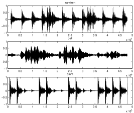
Figure 2: Sample data generated by a synthesizer (by courtesy of N.Murata).

Pseudo-observed data are generated by mixing the source by a random matrix,

$$A=I_{3}+S,$$ (5.2)

where each element of $S$ is distributed uniformly on $(-1/2,1/2)$. The residual crosstalk of the signals demixed by our method is $1.29\%$ on average. It takes about $122$ seconds (CPU time) for one hundred iteration of the same problem on our workstation. For reference, we have also solved the same demixing problem by the FastICA[Hurri et al.,1998]. In this case the residual crosstalk is $1.36\%$ on average and it takes about $156$ seconds for one hundred iteration on the same workstation. Since the author’s knowledge about the FastICA package is limited, one should not take this result seriously. It can, however, be said that our method is quite good also in practice.

6 Summary

We have constructed a new algorithm for finding a critical point of broad classes of cost functions on the orthogonal groups. This method is second-order-convergent since it is in essence the Newton method. The method here constructed is an extension (or a restriction) of the multiplicative updating method developed in our previous work[T.Akuzawa & N.Murata,1999]. The constraint for $\Delta$ from the nature of the orthogonal groups makes the problem a little complicated. We have, however, obtained a rigorous and explicit updating rule. We have also constructed a Levenberg-Marquardt-type variation, which is suitable for practical purpose. The global instability inherent in the Newton method is remedied in this version. Since our discussion does not depend on the detail of the cost function, this method is applicable to many concrete problems. The relatively mild assumption (2.1) on the form of the cost function, however, implies that our algorithm is especially suitable for the ICA. Its practical utility for the ICA have been illustrated here by a numerical simulation.

To summarize, our algorithm has numerous theoretical virtues such as the rigorous second order convergence, the explicit and strict formulation, and so on. It provides, also in practice, fast and powerful tools for the ICA and many other problems.

References

- [A.Hyvärinen,1997] A.Hyvärinen (1997). A Fast Fixed-Point Algorithm for Independent Component Analysis. Neural Computation, 9, 1483–1492.
- [B.W.Sliverman,1986] B.W.Sliverman (1986). Density Estimation for Statistics and Data Analysis. London: Chapman & Hall.
- [D.Cox,1985] D.Cox, D. (1985). A Penalty Method for Nonparametric Estimation of the Logarithmic Derivative of a Density Function. Ann.Inst.Statist.Math., 37, 271–288.
- [Hurri et al.,1998] Hurri, J., Gävert, H., Sälelä, J., & Hyvärinen, A. (1998). FastICA package for MATLAB. http://www.cis.hut.fi/projects/ica/fastica/.
-
[T.Akuzawa & N.Murata,1999]
T.Akuzawa & N.Murata (1999).
Multiplicative Nonholonomic/Newton -like Algorithm.
preprint
(available from http://www.islab.brain.riken.go.jp/~akuzawa/). - [W.H.Press et al.,1988] W.H.Press, B.P.Flannery, S.A.Teukolsky, & W.T.Vetterling (1988). Numerical Recipes in C. Cambridge: Cambridge U.P.