Brownian Particles far from Equilibrium

Abstract

We study a model of Brownian particles which are pumped with energy by means of a non-linear friction function, for which different types are discussed. A suitable expression for a non-linear, velocity-dependent friction function is derived by considering an internal energy depot of the Brownian particles. In this case, the friction function describes the pumping of energy in the range of small velocities, while in the range of large velocities the known limit of dissipative friction is reached. In order to investigate the influence of additional energy supply, we discuss the velocity distribution function for different cases. Analytical solutions of the corresponding Fokker-Planck equation in 2d are presented and compared with computer simulations. Different to the case of passive Brownian motion, we find several new features of the dynamics, such as the formation of limit cycles in the four-dimensional phase-space, a large mean squared displacement which increases quadratically with the energy supply, or non-equilibrium velocity distributions with crater-like form. Further, we point to some generalizations and possible applications of the model.

1 Introduction

As we know from classical physics, Brownian motion denotes the erratic motion of a small, but larger than molecular, particle in a surrounding medium, e.g. a gas or a liquid. This erratic motion results from the random impacts between the atoms or molecules of the medium and the (Brownian) particle, which cause changes in the direction and the amount of its velocity, $v$.

This type of motion would be rather considered as passive motion, simply because the Brownian particle does not play an active part in this motion. The Brownian particle keeps moving because the dissipation of energy caused by friction is compensated by the stochastic force, as expressed in the fluctuation-dissipation theorem (Einstein relation).

In this paper, we are particularly interested in the non-equilibrium motion of Brownian particles. The out-of-equilibrium state is reached by considering an additional influx of energy which is transfered into kinetic energy of the particles. This will be considered by a more complex friction coefficient, $\gamma_{0}$, which now can be a space- and/or velocity-dependent function, $\gamma(\mbox{\boldmath$r,v$})$, which can be also negative.

Negative friction is known i.e. from technical constructions, where moving parts cause a loss of energy, which is from time to time compensated by the pumping of mechanical energy. For example, in a mechanical clock the dissipation of energy by moving parts is compensated by a heavy weight. The weight stores potential energy, which is gradually transferred to the clock via friction, i.e. the strip with the weight is pulled down. Another example are violin strings, where friction-pumped oscillations occur, if the violin bow transfers energy to the string via friction. Already in the classical work “The Theory of Sound” of Lord Rayleigh considered motion with energy supply Ra45 .

Provided a supercritical influx of energy, passive motion could be transformed into active motion, which relies on the supply of energy from the surroundings. Active motion is of interest for the dynamics of driven systems, such as physico-chemical VaRoChYa87 ; DeDu71 ; DuDe74 ; Ge85 ; MiMe97 or biological SchiGr93 systems. However, recent models on self-driven particles often neglect the energetic aspects of active motion while focusing on the interaction of particles ViCzBeCoSh95 ; DeVi95 .

In order to describe active motion in the presence of stochastic forces, we have suggested a model of active Brownian particles, which have the ability to take up energy from the environment, to store it in an internal energy depot and to convert internal into kinetic energy SchwEbTi98 ; EbSchwTi99 ; SchwTiEb99 ; TiSchwEb99 ; EbErSchiSchw99 . Two of us have shown that these particles could move in an “high-velocity” or active mode, which results in different types of complex motion.

Other previous versions of active Brownian particle models consider also specific activities, such as environmental changes or signal-response behavior. In particular, the active Brownian particles are assumed to generate a self-consistent field which effects their further movement SchwSchi94 ; SchiMiRoMa95 ; Er99 . The non-linear feedback between the particles and the field generated by themselves may result in an interactive structure formation process on the macroscopic level. Hence, these models have been used to simulate a broad variety of pattern formations in complex systems, ranging from physical to biological and social systems La95 ; SchwLaFa97 ; HeSchwKeMo97 ; MiZa99 .

The main objective of this work is to study the influence of different types of non-linear friction terms on active Brownian particles and the corresponding probability distributions. Hence, we neglect possible environmental changes of the particles and rather focus on the energetic aspects of motion in the presence of noise. In Sect. 2, we introduce the idea of pumping by active friction and outline the basic dynamics of our model by means of Langevin and Fokker-Planck equations. Further, we investigate the distribution function for spatially uniform systems, i.e. in the absence of an external potential. In Sect. 3 we consider active Brownian motion in external potentials. For the case of a parabolic potential, we derive analytical expressions for the distribution function and present computer simulations based on the Langevin equation, which show the occurrence of limit cycles. The basic ideas are then generalized for other types of potentials. Finally, we discuss some possible applications for the dynamics of pumped Brownian particles.

2 Active Brownian Motion of Free Particles

2.1 Equations of Motion for Active Brownian Motion

The motion of a Brownian particle with mass $m$, position $r$, and velocity $v$ moving in a space-dependent potential, $U(\mbox{\boldmath$r$})$, can be described by the following Langevin equation:

$$\dot{\mbox{\boldmath$r$}}=\mbox{\boldmath$v$}\,;\,\,\dot{\mbox{\boldmath$v$}}=-\gamma(\mbox{\boldmath$v$})\,\mbox{\boldmath$v$}-\frac{1}{m}\mbox{\boldmath$\nabla$}U(\mbox{\boldmath$r$})+{\cal F}(t)$$ (1)

Here, $\gamma(\mbox{\boldmath$v$})$ is the friction coefficient, which is assumed to depend on velocity and and therefore implicitly on time. This rather general ansatz will allow us to consider more complex functions for the friction coefficient, as discussed below. ${\cal F}(t)$ is a stochastic force with strength $D$ and a $\delta$-correlated time dependence

$$\left\langle{\cal F}(t)\right\rangle=0\,;\,\,\left\langle{\cal F}(t){\cal F}(t^{\prime})\right\rangle=2D\,\delta(t-t^{\prime})$$ (2)

In the case of thermal equilibrium systems with $\gamma(\mbox{\boldmath$v$})=\gamma_{0}={\rm const.}$ we may assume that the loss of energy resulting from friction, and the gain of energy resulting from the stochastic force, are compensated in the average. In this case the fluctuation-dissipation theorem (Einstein relation) applies:

$$D=\gamma_{0}\frac{k_{B}T}{m}$$ (3)

$T$ is the temperature and $k_{B}$ is the Boltzmann constant.

In this paper we are mainly interested in the discussion of the probability density $P(\mbox{\boldmath$r$},\mbox{\boldmath$v$},t)$ to find the particle at location $r$ with velocity $v$ at time $t$. As well known, the distribution function $P(\mbox{\boldmath$r$},\mbox{\boldmath$v$},t)$ which corresponds to the Langevin Eq. (1), can be described by a Fokker-Planck equation of the form:

$$\frac{\partial P(\mbox{\boldmath$r$},\mbox{\boldmath$v$},t)}{\partial t} = \frac{\partial}{\partial\mbox{\boldmath$v$}}\left\{\gamma(\mbox{\boldmath$v$})\,\mbox{\boldmath$v$}\,P(\mbox{\boldmath$r$},\mbox{\boldmath$v$},t)+D\,\frac{\partial P(\mbox{\boldmath$r$},\mbox{\boldmath$v$},t)}{\partial\mbox{\boldmath$v$}}\right\}$$ (4)

$$-\mbox{\boldmath$v$}\,\frac{\partial P(\mbox{\boldmath$r$},\mbox{\boldmath$v$},t)}{\partial\mbox{\boldmath$r$}}+\frac{1}{m}\nabla U(\mbox{\boldmath$r$})\,\frac{\partial P(\mbox{\boldmath$r$},\mbox{\boldmath$v$},t)}{\partial\mbox{\boldmath$v$}}$$

In the special case $\gamma(\mbox{\boldmath$v$})=\gamma_{0}$ the stationary solution of Eq. (4), $P^{0}(\mbox{\boldmath$r$},\mbox{\boldmath$v$})$, is known to be the Boltzmann distribution:

$$P^{0}(\mbox{\boldmath$r$},\mbox{\boldmath$v$})=C\,\exp{\left(-\frac{U(\mbox{\boldmath$r$})}{k_{B}T}\right)}\;\exp{\left(-\frac{\gamma_{0}}{2\,D}\,\mbox{\boldmath$v$}^{2}\right)}$$ (5)

where the constant $C$ results from the normalization condition.

The major question discussed throughout this paper is how this known picture changes if we add a new degree of freedom to the model by considering that Brownian particles can be also pumped with energy from the environment. This extension leads to the model of active Brownian particles SchwSchi94 ; SchiMiRoMa95 ; EbSchwTi99 ; SchwEbTi98 . While the usual dynamic approach to Brownian motion is based on the assumption of a passive friction described by a constant, non-negative friction coefficient, $\gamma_{0}>0$, active Brownian motion considers active friction as an additional mechanism of the particle to gain energy. In the present model, this will be described by a more complex friction coefficient $\gamma(\mbox{\boldmath$v$})$ which is a velocity-dependent function. Several aspects of an additional space dependence were discussed in an earlier work SteEbCa94 .

In the next section, we will introduce two possible ansatzes for the pumping of energy, where the active friction depends on the velocity $v$ of the particle. In Sect. 2 we will restrict the discussion to the case $U(\mbox{\boldmath$r$})={\rm const.}$, but in Sect. 3 also the influence of external forces will be discussed. Further, from now on we will choose units in which $m\equiv 1$.

2.2 Pumping By Velocity-Dependent Friction

The velocity-dependent pumping of energy plays an important role e.g. in models of the theory of sound developed by Rayleigh Ra45 already at the end of the last century. In the simplest case we may assume the following friction function for the Brownian particle:

$$\gamma(\mbox{\boldmath$v$})=-\gamma_{1}+\gamma_{2}\,\mbox{\boldmath$v$}^{2}=\gamma_{1}\left(\frac{\mbox{\boldmath$v^{2}$}}{\mbox{\boldmath$v$}_{0}^{2}}-1\right)$$ (6)

This Rayleigh-type model is a standard model for self-sustained oscillations studied in different papers on nonlinear dynamics Kl94 ; MiZa99 . We note that

$$\mbox{\boldmath$v$}_{0}^{2}=\frac{\gamma_{1}}{\gamma_{2}}$$ (7)

defines a special value of the velocity where the friction function, Eq. (6), is zero (cf. Fig. 1).

Figure 1: Two different types of velocity dependent friction functions: (top) Rayleigh type, Eq. (6), (bottom) Eq. (8). Parameters: $\gamma_{1}=5$, $\gamma_{2}=1.4$, $\gamma_{0}=2$, $v_{0}=1.889$.

Another standard model for active Brownian dynamics with a zero $\mbox{\boldmath$v$}_{0}$ in the friction function introduced in SchiGr93 reads (cf. Fig. 1):

$$\gamma(\mbox{\boldmath$v$})=\gamma_{0}\left(1-\frac{v_{0}}{v}\right)$$ (8)

It has been shown that Eq. (8) allows to describe the active motion of different cell types, such as granulocytes SchiGr93 ; FrGr90 ; GrBu84 monocytes BoRaGr89 or neural crest cells GrNu91 . Here, the speed $v_{0}$ expresses the fact that the motion of cells is not only driven by stochastic forces, instead cells are also capable of active motion.

To compare Eqs. (6), (8) (cf. Fig. 1), we note that in both ansatzes we have a certain range of (small) velocities, where the friction coefficient can be negative, i.e. the motion of the particle can be pumped with energy. Due to the pumping mechanism, the conservation of energy clearly does not hold for the particle, i.e. we now have a strongly non-equilibrium canonical system FeEb89 .

Above a critical value of the velocity, described by $\mbox{\boldmath$v$}_{0}$, the active friction turns into passive friction again. In Eq. (6), the increase of the friction with increasing velocity is not bound to a maximum value. However, this is the case in Eq. (8), where the friction function converges into the constant of passive friction, $\gamma_{0}$, for large $v$. The disadvantage of Eq. (8), on the other hand, is the singularity of the friction function for $\mbox{\boldmath$v$}\to 0$. In Sect. 2.3, we will suggest a model of active friction which avoids these drawbacks, while providing a more general approach to derive a suitable function $\gamma(\mbox{\boldmath$v$})$.

But before, we want to discuss some features which result from the Rayleigh ansatz, Eq. (6). The stationary solution of the corresponding Fokker-Planck Eq. (4) reads in the isotropic case:

$$P^{0}(\mbox{\boldmath$v$})=C\exp\left(\frac{\gamma_{1}}{2D}\,\mbox{\boldmath$v$}^{2}-\frac{\gamma_{2}}{4D}\,\mbox{\boldmath$v$}^{4}\right)$$ (9)

The distribution $P^{0}(\mbox{\boldmath$v$})$, Eq. (9), has its maximum for $\mbox{\boldmath$v$}=0$, if $\gamma_{1}\leq 0$. For $\gamma_{1}>0$, the mean of the velocity distribution is still zero, but the maxima are different. Considering a two-dimension motion, the distribution then has the form of a hat (cf. also Fig. 3), indicating that the particle most likely moves with a constant absolute velocity $\mbox{\boldmath$v$}^{2}=\mbox{\boldmath$v$}_{0}^{2}=\gamma_{1}/\gamma_{2}$.

For the calculation of the normalization constant $C$ in Eq. (9) we use a method described by St67 and find with $\gamma_{2}=1$ the explicit expression Er97 :

$$C^{-1}=\pi\sqrt{\pi D}\;\exp\left(\frac{\gamma_{1}^{2}}{4D}\right)\left[1+{\rm erf}\left(\frac{\gamma_{1}}{2\sqrt{D}}\right)\right]$$ (10)

Using Eqs. (9), (10), we are able to calculate the different moments of the stationary velocity distribution and find:

$$\left\langle v^{2n}\right\rangle=\frac{(2D)^{n}}{Z_{2D}(\gamma_{1})}\;\frac{\partial^{n}}{\partial\gamma_{1}^{n}}\;Z_{2\mathrm{d}}(\gamma_{1})$$ (11)

with the function:

$$Z_{2\mathrm{d}}(\gamma_{1})=\pi\sqrt{\pi D}\;\exp\left(\frac{\gamma_{1}^{2}}{4D}\right)\left[1+{\rm erf}\left(\frac{\gamma_{1}}{2\sqrt{D}}\right)\right]$$ (12)

In particular, the second moment, which is proportional to the temperature, and the fourth moment which is proportional to the fluctuations of the temperature, read:

$$\left\langle\mbox{\boldmath$v$}^{2}\right\rangle = \gamma_{1}+\sqrt{\frac{D}{\pi}}\;\frac{2\exp\left(\frac{\displaystyle\gamma_{1}^{2}}{\displaystyle 4D}\right)}{1+{\rm erf}\left(\frac{\displaystyle\gamma_{1}}{\displaystyle 2\sqrt{D}}\right)}$$

$$\left\langle\mbox{\boldmath$v$}^{4}\right\rangle = \gamma_{1}^{2}+2D+\gamma_{1}\left\langle\mbox{\boldmath$v$}^{2}\right\rangle$$ (13)

We note that a similar discussion can be carried out also for the case of the friction function, Eq. (8). In this case the stationary solution of the Fokker-Planck Eq. (4) is of particular simplicity SchiGr93 :

$$P^{0}(\mbox{\boldmath$v$})=C\exp\left(\frac{\gamma_{0}}{2D}\,\left(v-v_{0}\right)^{2}\right)$$ (14)

In the following section, we will derive a model which allows us to generalize both special cases introduced here, so that the further discussion can be unified.

2.3 Pumping from an Internal Energy Depot

In order to avoid the drawbacks of the friction functions, Eqs. (6), (8), mentioned in the previous section, we need a friction function $\gamma(\mbox{\boldmath$v$})$ which does not diverge in the limit of small or large velocities. Further the case of the “normal” passive friction should be included as a limiting case. The ansatz suggested here is based on the recently developed model of Brownian motion with internal energy depot SchwEbTi98 ; EbSchwTi99 ; TiSchwEb99 ; SchwTiEb99 .

We assume that the Brownian particle should be able to take up external energy, which can be stored in an internal energy depot, $e(t)$. This energy depot may be may be altered by three different processes:

1. take-up of energy from the environment; where $q$ is the pump rate of energy,

2. internal dissipation, which is assumed to be proportional to the internal energy. Here the rate of energy loss, $c$, is assumed to be constant,

3. conversion of internal energy into motion, where $d\left(\mbox{\boldmath$v$}^{2}\right)$ is the rate of conversion of internal to kinetic degrees of freedom and $\eta\left(\mbox{\boldmath$v$}^{2}\right)$ is the efficiency of conversion. This means that the depot energy may be used to accelerate motion of the particle.

This extension of the model is motivated by investigations of active biological motion, which relies on the supply of energy. This energy can be dissipated by metabolic processes, but can be also converted into kinetic energy. The resulting balance equation for the internal energy depot of a pumped Brownian particle is then given by:

$$\frac{d}{dt}e(t)=q-c\;e(t)-\eta(\mbox{\boldmath$v$}^{2})d(\mbox{\boldmath$v$}^{2})\;e(t)$$ (15)

Generalizing the ansatz given in EbSchwTi99 ; SchwEbTi98 we postulate the following Langevin equation for the motion of Brownian particles with internal energy depot:

$$\dot{\mbox{\boldmath$v$}}+\gamma_{0}\mbox{\boldmath$v$}+\nabla U=\frac{\eta\left(\mbox{\boldmath$v$}^{2}\right)d\left(\mbox{\boldmath$v$}^{2}\right)}{\mbox{\boldmath$v$}^{2}}\;e(t)\mbox{\boldmath$v$}+{\cal F}(t)$$ (16)

Let us consider now two limiting cases:

(i) First, we assume

$$q(\mbox{\boldmath$r$})\equiv q_{0}\;;\quad d\left(\mbox{\boldmath$v$}^{2}\right)=d_{2}\mbox{\boldmath$v$}^{2}\;;\quad\eta\left(\mbox{\boldmath$v$}^{2}\right)\equiv 1$$ (17)

where $d_{2}>0$ is the conversion factor. Using the assumption of a fast relaxation of the internal energy depot we find the quasistationary value:

$$e_{0}=\frac{q_{0}}{c+d_{2}\mbox{\boldmath$v$}^{2}}$$ (18)

With the quasistationary approximation $e_{0}$, Eq. (18), the internal energy can be adiabatically eliminated, and we find the following effective friction function:

$$\gamma\left(\mbox{\boldmath$v$}^{2}\right)=\gamma_{0}-\frac{q_{0}\,d_{2}}{c+d_{2}\mbox{\boldmath$v$}^{2}}\;.$$ (19)

which is plotted in Fig. 2. We see that in the range of small velocities pumping due to negative friction occurs, as an additional source of energy for the Brownian particle. Hence, slow particles are accelerated, while the motion of fast particles is damped.

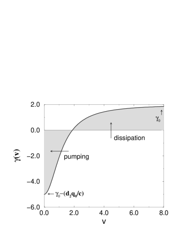
Figure 2: Velocity-dependent friction function $\gamma(v)$, Eq. (19) vs. velocity $v$. The velocity ranges for “pumping” ($\gamma(v)<0$) and “dissipation” ($\gamma(v)>0$) are indicated. Parameters: $q_{0}=10$; $c=1.0$; $\gamma_{0}=2$, $d_{2}=0.7$.

The friction function, Eq. (19), has again a zero, which reads in the considered case:

$$\mbox{\boldmath$v$}_{0}^{2}=\frac{q_{0}}{\gamma_{0}}-\frac{c}{d_{2}}$$ (20)

Eq. (19) agrees with the Rayleigh ansatz, Eq. (6), in the limit of rather small velocities, $\mbox{\boldmath$v$}\leq\mbox{\boldmath$v$}_{0}$. From the conditions $\gamma(\mbox{\boldmath$v$}=0)$ and $\gamma(\mbox{\boldmath$v$})=0$, we find for the two parameters of the Rayleigh ansatz:

$$-\gamma_{1}=\gamma_{0}-q_{0}\frac{d_{2}}{c}\;\;;\quad\gamma_{2}=\gamma_{0}\frac{d_{2}}{c}$$ (21)

Thus, the further discussion will also cover this case as long as $v\leq v_{0}$.

(ii) In the second limiting case we consider a very large energy depot which is then assumed to be constant, $e(t)=e_{0}={\rm const.}$ However, we may assume that the efficiency of conversion, $\eta\left(\mbox{\boldmath$v$}^{2}\right)$, decreases with increasing velocity as follows:

$$\eta\left(\mbox{\boldmath$v$}^{2}\right)=\frac{\eta_{1}}{1+\eta_{2}\mbox{\boldmath$v$}^{2}}$$ (22)

where $\eta_{1}$ and $\eta_{2}$ are constants. With $\eta_{0}=\eta_{1}d_{2}$, this case leads to the effective friction function TiSchwEb99 :

$$\gamma\left(\mbox{\boldmath$v$}^{2}\right)=\gamma_{0}-\frac{\eta_{0}\;e_{0}}{1+\eta_{2}\mbox{\boldmath$v$}^{2}}$$ (23)

Both expressions, Eq. (19) and Eq. (23), can be brought into the same form by defining some constants:

$$\gamma\left(\mbox{\boldmath$v$}^{2}\right) = \gamma_{0}\;\left[1-\frac{q^{\star}}{1+d^{\star}\mbox{\boldmath$v$}^{2}}\right]$$ (24)

$$q^{\star} = \frac{q_{0}d_{2}}{c\gamma_{0}}=\frac{\eta_{0}e_{0}}{\gamma_{0}}\;;\;d^{\star}=\frac{d_{2}}{c}=\eta_{2}$$ (25)

Using further the expression for the stationary velocity $\mbox{\boldmath$v$}_{0}^{2}$, Eq. (20), we find for Eq. (24)

$$\gamma\left(\mbox{\boldmath$v$}^{2}\right)=\gamma_{0}\;\frac{\left(\mbox{\boldmath$v$}^{2}-\mbox{\boldmath$v$}_{0}^{2}\right)}{(q_{0}/\gamma_{0})+\left(\mbox{\boldmath$v$}^{2}-\mbox{\boldmath$v$}_{0}^{2}\right)}$$ (26)

We restrict the further discussion to the two-dimensional space $\mbox{\boldmath$r$}=\{x_{1},x_{2}\}$. Then the stationary velocities $v_{0}$, Eqs. (7), (20), where the friction is just compensated by the energy supply, define a cylinder in the four-dimensional space:

$$v_{1}^{2}+v_{2}^{2}=\mbox{\boldmath$v$}_{0}^{2}$$ (27)

which attracts all deterministic trajectories of the dynamic system. The stationary solution of the Fokker-Planck Eq. (4) reads for the friction function, Eq. (19), and in the absence of an external potential, i.e. $U(x_{1},x_{2})\equiv 0$:

$$P^{0}(\mbox{\boldmath$v$})=C^{\prime}\,\left(1+\frac{d_{2}\mbox{\boldmath$v$}^{2}}{c}\right)^{\frac{q_{0}}{2D}}\;\exp{\left(-\frac{\gamma_{0}}{2D}\,v^{2}\right)}$$ (28)

Compared to Eq. (5), which describes the Maxwellian velocity distribution of “simple” Brownian particles, a new prefactor appears now in Eq. (28) which results from the internal energy depot. In the range of small values of $v^{2}$, the prefactor can be expressed by a power series truncated after the first order, and Eq. (28) reads then:

$$P^{0}(\mbox{\boldmath$v$})\sim\exp{\left[-\frac{\gamma_{0}}{2D}\left(1-\frac{q_{0}d_{2}}{c\gamma_{0}}\right)\,\mbox{\boldmath$v$}^{2}+\cdots\right]}$$ (29)

In Eq. (29), the sign of the expression in the exponent depends significantly on the parameters which describe the balance of the energy depot. For a subcritical pumping of energy, $q_{0}d_{2}<c\gamma_{0}$, the expression in the exponent is negative and an unimodal velocity distribution results, centered around the maximum $\mbox{\boldmath$v$}_{0}=0$. This is the case of the “low velocity” or passive mode for the stationary motion which here corresponds to the Maxwellian velocity distribution. However, for supercritical pumping,

$$q_{0}d_{2}>c\gamma_{0}$$ (30)

the exponent in Eq. (29) becomes positive, and a crater-like velocity distribution results. This is also shown in Fig. 3. The maxima of $P^{0}(\mbox{\boldmath$v$})$ correspond to the solutions for $\mbox{\boldmath$v$}_{0}^{2}$, Eq. (20). The corresponding “high velocity” or active mode SchwTiEb99 for the stationary motion is described by strong deviations from the Maxwell distribution.

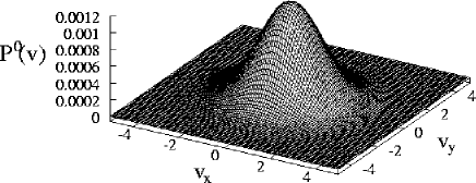
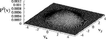
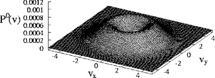
Figure 3: Normalized stationary solution $P^{0}(\mbox{\boldmath$v$})$, Eq. (28), for $d_{2}=0.07$ (top), $d_{2}=0.2$ (middle) and $d_{2}=0.7$ (bottom). Other parameters: $\gamma_{0}=2$, $D=2$, $c=1$, $q_{0}=10$. Note that $d_{2}=0.2$ is the bifurcation point for the given set of parameters.

2.4 Investigation of two Limit Cases

In the limit of strong noise $D\sim T\rightarrow\infty$, i.e. at high temperatures, we get from Eq. (28) the known Maxwellian distribution by means of Eq. (3):

$$P^{0}(\mbox{\boldmath$v$})=\left(\frac{1}{2\pi k_{B}T}\right)\;\exp\left(-\frac{\mbox{\boldmath$v$}^{2}}{2k_{B}T}\right)$$ (31)

which corresponds to standard Brownian motion in two dimensions. Hence, many characteristic quantities are explicitly known as e.g. the dispersion of the velocities

$$\left\langle\mbox{\boldmath$v$}^{2}\right\rangle=2k_{B}T$$ (32)

and the Einstein relation for mean squared displacement

$$\left\langle\Big{(}\mbox{\boldmath$r$}(t)-\mbox{\boldmath$r$}(0)\Big{)}^{2}\right\rangle=4\frac{k_{B}T}{\gamma_{0}}\,t$$ (33)

In the other limiting case of strong activation, i.e. relatively weak noise $D\sim T\rightarrow 0$ and/or strong pumping, we find a $\delta$-distribution instead:

$$P^{0}(\mbox{\boldmath$v$})=C\delta\left(\mbox{\boldmath$v$}^{2}-\mbox{\boldmath$v$}_{0}^{2}\right)\;;\quad\left\langle\mbox{\boldmath$v$}^{2}\right\rangle=\mbox{\boldmath$v$}_{0}^{2}$$ (34)

In order to treat this case in the full phase space, we follow SchiGr93 ; MiMe97 and introduce first an amplitude-phase representation in the velocity-space:

$$v_{1}=v_{0}\,\cos{(\varphi)}\;;\quad v_{2}=v_{0}\,\sin{(\varphi)}$$ (35)

This allows us to separate the variables and we get a distribution function of the form:

$$P(x_{1},x_{2},v_{1},v_{2},t)=P(x_{1},x_{2},t)\cdot\delta(v_{1}^{2}+v_{2}^{2}-v_{0}^{2})\cdot P\left(\varphi,t\right)$$ (36)

The distribution of the phase $\varphi$ satisfies the Fokker-Planck equation:

$$\frac{\partial}{\partial t}P\left(\varphi,t\right)=D_{\varphi}\frac{\partial^{2}}{\partial\varphi^{2}}P\left(\varphi,t\right)$$ (37)

By means of the known solution of Eq. (37) we get for the mean square:

$$\left\langle\varphi^{2}(t)\right\rangle=D_{\varphi}t\;;\quad D_{\varphi}=\frac{D}{v_{0}^{2}}$$ (38)

where $D_{\varphi}$ is the angular diffusion constant. By means of this, the mean squared spatial displacement $\left\langle r^{2}(t)\right\rangle$ of the particle can be calculated according to MiMe97 as:

$$\left\langle r^{2}(t)\right\rangle=\frac{2v_{0}^{4}t}{D}+\frac{v_{0}^{6}}{D^{2}}\left[\exp\left(-\frac{2Dt}{v_{0}^{2}}\right)-1\right]$$ (39)

For times $t\gg v_{0}^{2}/D$, we find from Eq. (39) the following expression for the effective spatial diffusion constant:

$$D_{r}^{\rm eff}=\frac{2v_{0}^{4}}{D}=\frac{2}{D}\left(\frac{q_{0}}{\gamma_{0}}-\frac{c}{d_{2}}\right)^{2}$$ (40)

where $v_{0}$, Eq. (20), considers the additional pumping of energy resulting from the friction function, $\gamma(\mbox{\boldmath$v$})$. Due to this additional pumping, we obtain a high sensitivity with respect to noise expressed in the scaling with $(1/D)$.

3 Active Brownian Motion in External Potentials

3.1 Motion in a Parabolic Potential

In the following, we discuss the motion in a two-dimensional external potential, $U(x_{1},x_{2})$, which results in additional forces on the pumped Brownian particle. The case of a constant external force was experimentally and theoretically investigated in SchiGr93 . Here we concentrate first on a simple non-linear potential:

$$U(x_{1},x_{2})=\frac{1}{2}a\,(x_{1}^{2}+x_{2}^{2})$$ (41)

If we for the moment restrict the discussion to a deterministic motion, the dynamics will be described by four coupled first-order differential equations:

$$\begin{array}[]{rcl}\dot{x}_{1}=v_{1}&&\dot{v}_{1}=-\gamma\left(v_{1},v_{2}\right)v_{1}-ax_{1}\\ \dot{x}_{2}=v_{2}&&\dot{v}_{2}=-\gamma\left(v_{1},v_{2}\right)v_{2}-ax_{2}\end{array}$$

For the one-dimensional Rayleigh model it is well known that this system processes a limit cycle corresponding to sustained oscillations with the energy $E_{0}=\gamma_{1}/\gamma_{2}$. For the two-dimensional case we have shown EbSchwTi99 that limit cycles occur in the four-dimensional space. The projection of this periodic motion to the $\{v_{1},v_{2}\}$ plane is again the cylinder, defined by Eq. (27). The projection to the $\{x_{1},x_{2}\}$ plane corresponds to a circle

$$x_{1}^{2}+x_{2}^{2}=r_{0}^{2}={\rm const.}$$ (42)

The energy for motions on the limit cycle is:

$$E_{0}=\frac{1}{2}(v_{1}^{2}+v_{2}^{2})+\frac{a}{2}(x_{1}^{2}+x_{2}^{2})=\frac{1}{2}v_{0}^{2}+\frac{a}{2}r_{0}^{2}$$ (43)

In EbSchwTi99 we have shown that any initial value of the energy converges (at least in the limit of strong pumping) to

$$H\longrightarrow E_{0}=v_{0}^{2}$$ (44)

This corresponds to an equal distribution between kinetic and potential energy. As for the harmonic oscillator in one dimension, both parts contribute the same amount to the total energy. This result was obtained in EbSchwTi99 using the assumption that the energy is a slow (adiabatic) variable which allows a phase average with respect to the phases of the rotation.

In explicite form we may represent the motion on the limit cycle in the four-dimensional space by the four equations:

$$\begin{array}[]{rcl}x_{1}=r_{0}\,\cos(\omega t+\varphi_{0})&&v_{1}=-r_{0}\,\omega\,\sin(\omega t+\varphi_{0})\\ x_{2}=r_{0}\,\sin(\omega t+\varphi_{0})&&v_{2}=r_{0}\,\omega\,\cos(\omega t+\varphi_{0})\end{array}$$

The frequency $\omega$ is given by the time the particle needs for one period while moving on the circle with radius $r_{0}$ with constant speed $v_{0}$. This leads to the relation

$$\omega_{0}=\frac{v_{0}}{r_{0}}=\sqrt{a}=\omega$$ (45)

This means that even in the case of strong pumping the particle oscillates with the frequency given by the linear oscillator frequency $\omega$.

The trajectory defined by the four equations (3.1) is like a hoop in the four-dimensional space. Therefore, most projections to the two-dimensional subspaces are circles or ellipses. However there are two subspaces, namely $\{x_{1},v_{2}\}$ and $\{x_{2},v_{1}\}$, where the projection is like a rod.

A second limit cycle is obtained by time reversal:

$$t\rightarrow-t;\quad v_{1}\rightarrow-v_{1};\quad v_{2}\rightarrow-v_{2}$$ (46)

This limit cycle also forms a hula hoop which is different from the first one in that the projection to the $\{x_{1},x_{2}\}$ plane has the opposite rotation direction compared to the first one. However both limit cycles have the same projections to the $\{x_{1},x_{2}\}$ and to the $\{v_{1},v_{2}\}$ plane. The separatrix between the two attractor regions is given by the following plane in the four-dimensional space:

$$v_{1}+v_{2}=0$$ (47)

Applying similar arguments to the stochastic problem we find that the two hoop-rings are converted into a distribution looking like two embracing hoops with finite size, which for strong noise converts into two embracing tires in the four-dimensional space EbErSchiSchw99 . The projections of the distribution to the $\{x_{1},x_{2},v_{2}\}$ subspace and to the $\{v_{1},v_{2},x_{2}\}$ subspace are two-dimensional rings as shown in Fig. 4. While in the deterministic case either left- or righthanded rotations are found, in the stochastic case the system may switch randomly between the left- and righthand rotations, since the separatrix becomes penetrating (see Fig. 5). This can be also confirmed by looking at the projections of the distribution to the $\{x_{1},v_{2}\}$ plane and the $\{x_{2},v_{1}\}$ plane (cf. Fig. 6). Since the hula hoop distribution intersects perpendicular the $\{x_{1},v_{2}\}$ and the $\{x_{2},v_{1}\}$ plane, the projections to these planes are rod-like and the intersection manifold with these planes consists of two ellipses located in the diagonals of the planes.

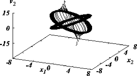
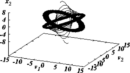
Figure 4: Projections of a stochastic trajectory on the three-dimensional subspaces $\{x_{1},x_{2},v_{2}\}$ and $\{x_{1},x_{2},v_{2}\}$ for very low noise ($D=0.01$). The particle will not leave the attractor which was reached dependant on the initial conditions (One of the trajectories represents righthanded and the other on lefthanded rotations). The trajectories were obtained with long time computer simulations of Eq. (16) with constant energy depot, Eq. (18). Other parameters: $\gamma_{0}=0.2$, $c=0.01$, $d_{2}=0.1$, $a=2.0$ and $q_{0}=10.0$.

Figure 5: Projections of a stochastic trajectory on the three-dimensional subspaces $\{x_{1},x_{2},v_{2}\}$ and $\{x_{1},x_{2},v_{2}\}$ for strong noise ($D=0.8$). Other parameters see Fig. 4.

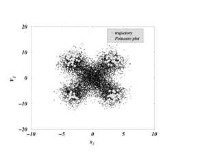
Figure 6: Poincaré plots and projections of a stochastic trajectory on the two-dimensional subspaces $\{x_{1},v_{2}\}$ and $\{x_{2},v_{1}\}$ (same simulation as in Fig. 4). The noise strength is large enough to allow one particle to penetrate the separatrix between the two hula-hoop-like attractors in finite time. For smaller noise one would need to simulate the particle’s motion with different initial conditions to reach both hoops/tires.

In order to get the explicite form of the distribution we may introduce the amplitude-phase representation

$$\begin{array}[]{rcl}x_{1}=\varrho\,\cos(\omega t+\varphi)&&v_{1}=-\varrho\,\omega\,\sin(\omega t+\varphi)\\ x_{2}=\varrho\,\sin(\omega t+\varphi)&&v_{2}=\varrho\,\omega\,\cos(\omega t+\varphi)\end{array}$$ (48)

where the radius $\varrho$ is now a slow stochastic variable and the phase $\varphi$ is a fast stochastic variable. By using the standard procedure of averaging with respect to the fast phases we get for the Rayleigh model of pumping, Eq. (6), the following distribution of the radii:

$$P_{0}(\varrho) \simeq \exp{\left[2\,\frac{\gamma_{1}}{D}a\varrho^{2}\left(1-\frac{\varrho^{2}}{r_{0}^{2}}\right)\right]}$$ (49)

$$r_{0}^{2} = \frac{v_{0}^{2}}{\omega^{2}}=\frac{\gamma_{1}}{a\gamma_{2}}$$

This distribution has its maximum value at $\varrho=r_{0}$.

For the friction function Eq. (19) resulting from the depot model, we get the following stationary solution for the distribution of the radii:

$$P_{0}(\varrho)\simeq\left(1+\frac{d_{2}}{c}a\varrho^{2}\right)^{\frac{q_{0}}{2D}}\exp{\left(-\frac{\gamma_{0}}{D}a\varrho^{2}\right)}$$ (50)

Again, we find that the maximum is located at:

$$\varrho^{2}=r_{0}^{2}=\frac{v_{0}^{2}}{\omega^{2}}=\left(\frac{q_{0}}{\gamma_{0}}-\frac{c}{d_{2}}\right)\frac{1}{\omega^{2}}$$ (51)

Due to the special form of the attractor which consists, as pointed out above, of two hula hoops embracing each other, the distribution in the phase space cannot be constant at $\varrho={\rm const.}$ An analytical expression for the distribution in the four-dimensional phase space is not yet available. But it is expected that the probability density is concentrated around the two deterministic limit cycles.

3.2 Generalization for Other Potentials

For the harmonic potential discussed above the equal distribution between potential and kinetic energy, $mv_{0}^{2}=ar_{0}^{2}$, is valid, which leads to the relation: $\omega_{0}=v_{0}/r_{0}=\omega$. For other radially symmetric potentials $U(r)$, this relation has to be replaced by the condition that on the limit cycle the attracting radial forces are in equilibrium with the centrifugal forces. This condition leads to

$$\frac{v_{0}^{2}}{r_{0}}=|U^{\prime}(r_{0})|$$ (52)

For a given $v_{0}$, this equation defines an implicit relation for the the equilibrium radius $r_{0}$, namely: $v_{0}^{2}=r_{0}\,|U^{\prime}(r_{0})|$. Then the frequency of the limit cycle oscillations is given by

$$\omega_{0}^{2}=\frac{v_{0}^{2}}{r_{0}^{2}}=\frac{|U^{\prime}(r_{0})|}{r_{0}}$$ (53)

In the case of linear oscillators this leads to $\omega_{0}=\sqrt{a}$ as before, Eq. (45). But e.g. for the case of a quartic potential

$$U(r)=\frac{k}{4}r^{4}$$ (54)

we get the limit cycle frequency

$$\omega_{0}=\frac{k^{1/4}}{v_{0}^{1/2}}$$ (55)

If Eq. (52) has several solutions for the equilibrium radius $r_{0}$, the dynamics might be much more complicated, e.g. we could find Kepler-like orbits oscillating between the solutions for $r_{0}$. In other words, we then find – in addition to the driven rotations already mentioned – also driven oscillations between the multiple solutions of Eq. (52).

In the general case of potentials $U\left(x_{1},x_{2}\right)$ which do not obey a radial symmetry, the local curvature of potential levels $U\left(x_{1},x_{2}\right)={\rm const.}$ replaces the role of the radius $r_{0}$. We thus define $\varrho_{U}\left(x_{1},x_{2}\right)$ as the radius of the local curvature. In general, the global dynamics will be very complicated, however the local dynamics can be described as follows: Most particles will move with constant kinetic energy

$$\mbox{\boldmath$v$}^{2}=v_{1}^{2}+v_{2}^{2}=v_{0}^{2}={\rm const.}$$ (56)

along the equipotential lines, $U\left(x_{1},x_{2}\right)={\rm const.}$ In dependence on the initial conditions two nearly equally probable directions of the trajectories, a counter-clockwise and a clockwise direction, are possible. Among the different possible trajectories the most stable will be the one which fulfills the condition that the potential forces and centrifugal forces are in equilibrium:

$$v_{0}^{2}=\varrho_{U}\left(x_{1},x_{2}\right)\left|\nabla U\left(x_{1},x_{2}\right)\right|$$ (57)

This equation is a generalization of Eq. (52).

4 Discussion and Conclusion

An interesting application of the theoretical results given above, is the following: Let us imagine a system of active Brownian particles which are pairwise bound by a potential $U(r_{1}-r_{2})$ to dumb-bell-like configurations. Thus, the pairs of active particles could be regarded as “active Brownian molecules”. Then the motion of each “molecule” consists of two independent parts: the free motion of the center of mass and the relative motion under the influence of the potential.

The motion of the center of mass is described by the equations given in Sect. 2, while the relative motion is described by the equations given in Sect. 3. As a consequence, the center of mass of the dumb-bell will perform a driven Brownian motion, but in addition the dumb-bell is driven to rotate around the center of mass. We then observe that a system of pumped Brownian molecules – with respect to their center of mass velocities – has a distribution corresponding to Eq. (9) or Eq. (28). However, since the internal degrees of freedom are excited, we also observe driven rotations and in general (if Eq. (52) has at least two solutions) also driven oscillations. Thus, we conclude that the mechanisms described here may be used also to excite the internal degrees of freedom of Brownian molecules.

Another possible application is the motion of clusters of active Brownian molecules. Similar to the case of the dumb-bells, these clusters are driven by the take-up of energy to perform spontaneous rotations. Eventually, a stationary state will be reached which is a mixture of rotating clusters or droplets, respectively.

These suggested applications for the dynamics of pumped Brownian particles will of course need further investigations. In this paper the aim was rather to study the influence of non-linear friction terms on Brownian particles from a more general perspective.

A suitable expression for a non-linear, velocity-dependent friction function $\gamma(\mbox{\boldmath$v$})$ has been obtained by considering an internal energy depot of the Brownian particles. This energy depot can be changed by energy take-up, internal dissipation and conversion of internal into kinetic energy. Provided a fast relaxation, the depot can be described by a quasistationary value. We then found that the velocity-dependent friction function describes the pumping of energy in the range of small velocities, while in the range of large velocities the known limit of (dissipative) friction is reached.

In this paper, the focus was on the distribution function of pumped Brownian particles. Therefore, in addition to the mechanisms of pumping, we had to consider the dependence on stochastic influences, namely on the strength of the stochastic force, $D$. We could find new dynamical features for pumped Brownian particles, such as:

1. new diffusive properties with large mean squared displacement, which increases quadratically with the energy supply and scales with the noise intensity as $1/D$

2. non-equilibrium velocity distributions with crater-like shape,

3. the formation of limit cycles corresponding to left/righthand rotations,

4. the switch between these opposite directions, i.e. the penetration of the separation, during the stochastic motion of a pumped Brownian particle.

Qualitative similar features are obtained for the motion of driven particles in physico-chemical systems, for example for the motion of liquid droplets on hot surfaces, or the motion of surface-active solid particles DeDu71 ; DuDe74 ; Ge85 ; MiMe97 . There are also relations to active biological motion SchiGr93 ; EbSchwTi99 . In this paper, we did not intend to model any particular object but analyzed the general physical non-equilibrium properties of such systems. While our investigations are based on rather simple physical assumptions on non-linear friction for Brownian particles, we found a rich dynamics, which might be of interest for more applied investigations later.

References

- (1) J. W. Rayleigh, The Theory of Sound, volume I, Dover, New York, 2 edition, 1945.
- (2) V. A. Vasiliev, Y. M. Romanovsky, D. S. Chernavsky, and V. G. Yakhno, Autowave Processes in Kinetic Systems, Dt. Verlag der Wissenschaften, Berlin, 1987.
- (3) B. V. Derjagin and S. S. Dukhin, in Research in Surface Forces, edited by B. V. Derjagin, volume 3, page 269, Consulatants Bureau, 1971.
- (4) S. S. Dukhin and B. V. Derjagin, in Surface and Colloidal Science, edited by E. Matiejevic, volume 7, page 322, Wiley, 1974.
- (5) P. G. de Gennes, Review of Modern Physics 57, 827 (1985).
- (6) A. S. Mikhailov and D. Meinköhn, Self-motion in physico-chemical systems far from thermal equilibrium, in Stochastic Dynamics, edited by L. Schimansky-Geier and T. Pöschel, volume 484 of Lecture Notes in Physics, pages 334–345, Springer, Berlin, 1997.
- (7) M. Schienbein and H. Gruler, Bull. Mathem. Biology 55, 585 (1993).
- (8) T. Vicsek, A. Czirok, E. Ben-Jacob, I. Cohen, and O. Shochet, Physical Review Letters 75, 1226 (1995).
- (9) I. Derényi and T. Vicsek, Physical Review Letters 75, 374 (1995).
- (10) F. Schweitzer, W. Ebeling, and B. Tilch, Physical Review Letters 80, 5044 (1998).
- (11) W. Ebeling, F. Schweitzer, and B. Tilch, BioSystems 49, 17 (1999).
- (12) F. Schweitzer, B. Tilch, and W. Ebeling, Europhysics Journal B (1999), in press.
- (13) B. Tilch, F. Schweitzer, and W. Ebeling, Physica A 273, 294 (1999).
- (14) W. Ebeling, U. Erdmann, L. Schimansky-Geier, and F. Schweitzer, Complex motion of brownian particles with energy supply, in Proceedings of the International Conference “Stochastic and Chaotic Dynamics in the Lakes”, edited by P. V. E. McClintock, American Institute of Physics, 1999, in press.
- (15) F. Schweitzer and L. Schimansky-Geier, Physica A 206, 359 (1994).
- (16) L. Schimansky-Geier, M. Mieth, H. Rosé, and H. Malchow, Physica A 207, 140 (1995).
- (17) U. Erdmann, Interjournal of Complex Systems 114 (1999), Article.
- (18) L. Lam, Chaos, Solitons & Fractals 6, 267 (1995).
- (19) F. Schweitzer, K. Lao, and F. Family, BioSystems 41, 153 (1997).
- (20) D. Helbing, F. Schweitzer, J. Keltsch, and P. Molnár, Physical Review E 56, 2527 (1997).
- (21) A. S. Mikhailov and D. Zanette, Physical Review E 60, 4571 (1999).
- (22) O. Steuernagel, W. Ebeling, and V. Calenbuhr, Chaos, Solitons & Fractals 4, 1917 (1994).
- (23) Y. L. Klimontovich, Physics-Uspekhi 37, 737 (1994).
- (24) K. Franke and H. Gruler, Europ. Biophys. J. 18, 335 (1990).
- (25) H. Gruler and B. Bültmann, Blood Cells 10, 61 (1984).
- (26) A. d. Boisfleury-Chevance, B. Rapp, and H. Gruler, Blood Cells 15, 315 (1989).
- (27) H. Gruler and R. Nuccitelli, Cell Mot. Cytoskel. 19, 121 (1991).
- (28) R. Feistel and W. Ebeling, Evolution of Complex Systems. Self-Organization, Entropy and Development, Kluwer, Dordrecht, 1989.
- (29) R. L. Stratonovich, Topics in the Theory of Random Noise, volume vol II, Gordon and Breach, London, 1967.
- (30) U. Erdmann, Ensembles von van-der-Pol-Oszillatoren, Master’s thesis, Humboldt University, Berlin, 1997.