Non-equilibrium tunneling into general quantum Hall edge states

Abstract

In this paper we formulate the theory of tunneling into general Abelian fractional quantum Hall edge states. In contrast to the simple Laughlin states, a number of charge transfer processes must be accounted for. Nonetheless, it is possible to identify a unique value corresponding to dissipationless transport as the asymptotic large-$V$ conductance through a tunneling junction, and find fixed points (CFT boundary conditions) corresponding to this value. The symmetries of a given edge tunneling problem determine the appropriate boundary condition, and the boundary condition determines the strong-coupling operator content and current noise.

I Introduction

Tunneling into the edges of fractional quantum Hall (FQH) states is important as the most experimentally accessible probe of the fractionally charged quasiparticles believed to exist in bulk FQH states. Although a large body of work has been carried out on tunneling between edges of Laughlin states, and more generally on tunneling between Luttinger liquids, a theoretical understanding of tunneling into general FQH states is still missing beyond weak coupling, where the comparison to experiment is puzzling. As opposed to the edges of Laughlin states ($\nu=\frac{1}{2q+1}$), general Abelian edge states such as the main sequence $\nu=\frac{p}{2pq+1}$ contain several quasiparticle and electron operators and thus multiple tunneling processes transferring different amounts of charge. The purpose of this paper is to develop a framework to study this multiple tunneling problem.

The chiral-Luttinger-liquid ($\chi$LL) model [1] for incompressible filling fractions [2, 3] and a composite-fermion theory for compressible states [4] both predict that the tunneling exponent $\alpha$ in $I\propto V^{\alpha}$ for tunneling into FQH edges has a plateau structure as a function of $\nu$. Experiments by Grayson et. al. [5] show a smooth dependence $\alpha\approx\nu^{-1}$ for most samples, although some samples do show a plateau structure near $\nu=1/3$ [6]. Different theoretical scenarios have emerged [7], some predicting $\alpha=\nu^{-1}$. The natural question to ask is whether these theories will also endure other experimental tests. More precisely, these theories share the same weak-coupling predictions, but will not necessarily agree at strong coupling. In this paper we describe the strong coupling physics for the $\chi$LL theory of edge states and show that the resulting value of large-$V$ conductance corresponds to a dissipationless zero-temperature fixed point. The result should be comparable to experiments on point tunneling between quantum Hall states and to other candidate theories.

The single-edge tunneling problem is known to contain a great deal of interesting physics. In tunneling between two $\nu=1/3$ edges, there are two starting points: electron ($e$) or quasiparticle ($e^{*}=e/3$) tunneling. These two regimes are connected by a weak-strong duality symmetry. In each regime, there is only a single tunneling process (or operator) that transfers the respective charge. An exact solution [8] via the thermodynamic Bethe ansatz describes completely the crossover between these two pictures, along the integrable trajectory. In tunneling between edges of the two-mode hierarchy state $\nu=2/5$, there are two most relevant electron operators (charge $e$ and fermionic statistics) in each edge, and consequently four ways to transfer charge $e$ between the edges. At strong coupling there are both charge $e/5$ and charge $2e/5$ quasiparticles which can tunnel from one edge to the other. We will show that the important properties (conductance, noise, operator content) near the strong-coupling fixed point can be determined without an exact solution for the crossover.

Just as interesting as tunneling between edges of the same FQH state is the “mismatched” problem of tunneling between different filling fractions $\nu_{1},\nu_{2}$ [9, 10], where new effective fractional charges appear in the strongly coupled system in the single-mode case [11]; this case includes tunneling from a metal (which can be modeled by the Fermi liquid $\nu=1$ state) to a FQH state. In this problem, like in the case of same edge tunneling, the hierachical edge states contain several electron operators, and therefore there are many ways of transferring charge from the Fermi liquid reservoir to the FQH edges.

In this paper we address the problem of tunneling between hierachical edge modes, using different approaches. We start by giving in section II an elementary argument that two values of the junction conductance correspond to dissipationless transport, and determine the boundary conditions on bosonic modes in the $\chi$LL theory which correspond to these conductances. Then a conformal field theory calculation of the partition function is used in section III to justify the strong-coupling duality picture of instantons between different minima of the tunneling operators. This calculation determines the operator content at strong coupling, which determines the noise and corrections to the tunneling current. These corrections could in principle distinguish among different candidate theories, even when they share the same asymptotic large-voltage conductance. Section IV contains a brief summary of our results.

II Large-voltage conductance

In this section we focus on the aymptotic large-voltage conductance for a general junction between two FQH states. We start with an elementary argument based on energy conservation, and show that the value suggested by this argument corresponds to specific boundary conditions on the neutral modes in the $\chi$LL theory. “Neutral modes” here refers to those which do not carry charge in their action on the complete system of two edges. For example, a mode which adds charge to one edge and removes an equal charge from the other is a neutral mode of the whole system, even though its restriction to either edge is charged. In other words, neutral modes of the combined two-edge system need not be combinations of neutral modes from each multi-mode subedge; they may also include charged modes from each subedge, as long as the total charge is zero.

A Dissipation and conductance

A simple argument shows that an upper bound on the conductance through a junction between FQH edges follows from the assumption that only one mode on each edge couples to the electric potential. In the $\chi$LL theory, this assumption holds in the presence of either unscreened Coulomb interactions or random hopping at the edge, for both nonchiral [2] and chiral [12] edges. Since in experiments the Coulomb interaction is screened only at moderate distances, and impurities are present, we assume separation of charge and neutral modes on each edge. The currents labeled in Fig. 1 are $I_{1}=\nu_{1}V_{1},I_{2}=\nu_{2}V_{2},I_{1}^{\prime}=\nu_{1}V_{1}^{\prime},I_{2}^{\prime}=\nu_{2}V_{2}^{\prime}$ (here $\frac{e^{2}}{h}=1$). Current and energy conservation at the junction give

$$\nu_{1}(V_{1}-V_{1}^{\prime})+\nu_{2}(V_{2}-V_{2}^{\prime}) = 0$$ (1)

$$\nu_{1}(V_{1}^{2}-{V_{1}^{\prime}}^{2})+\nu_{2}(V_{2}^{2}-{V_{2}^{\prime}}^{2}) = 2P.$$ (2)

Here $P$ is the power dissipated at the junction. In terms of the two-terminal conductance $g=I_{\rm t}/(V_{1}-V_{2})=I_{\rm t}/V$,

$$P=g^{2}V^{2}\left[{1\over g}-{{\nu_{1}}^{-1}+{\nu_{2}}^{-1}\over 2}\right].$$ (3)

FIG. 1.: Schematic geometry for point tunneling between quantum Hall states.

The dissipated power is zero for $g=0$ or $g=\sigma_{hm}=2\nu_{1}\nu_{2}/(\nu_{1}+\nu_{2})$, and positive for intermediate values; energy conservation forbids values $g\geq\sigma_{hm}$. The dissipated power can go into excitations of the oscillator modes of the outgoing edges [10]. The currently known fixed points for tunneling between quantum Hall edges all have zero dissipation at zero temperature except in the presence of exactly marginal operators (as in tunneling between $\nu=1$ states). We thus conjecture that, unless marginal tunneling operators are present, the conductance saturates for large $V_{1}-V_{2}$ at the value $\sigma_{hm}$.

B Boundary conditions and conductance

The two values of the dissipationless tunneling conductance result from imposing either Neumann ($N$) or Dirichlet ($D$) boundary conditions on one of the neutral bosonic modes in the $\chi$LL theory of the combined (two-edge) system. The $N$ condition corresponds to no tunneling in the geometry of Fig. 1, hence $g=0$, whereas the $D$ condition saturates the upper bound $g=\sigma_{\rm hm}$. There can be several boundary conditions with the same value of conductance: these differ in the conformally invariant boundary conditions of other neutral modes and in operator content. The total charge mode always has $N$ boundary condition from charge conservation.

An edge of a state with $n$ condensates is described by a universal $n\times n$ matrix $K$ and charge $n$-vector ${\bf t}$ inherited from the bulk Chern-Simons effective theory. For chiral edges (all modes propagate in the same direction), $K$ is positive definite and the scaling dimension of the vertex operator $O_{\bf m}=\exp(im_{j}\phi_{j})$ is $\Delta({\bf m})=\frac{1}{2}{\bf m}^{\rm T}K^{-1}{\bf m}$. For nonchiral edges such as $\nu=2/3$, the same holds but with $K^{-1}$ replaced by the scaling-dimension matrix $\Delta$ [2, 3]. Define an enlarged $n_{K}$-dimensional $K$-matrix ($n_{K}=n_{1}+n_{2}$) that combines both edges, one with an $n_{1}\times n_{1}$ matrix $K_{1}$ and the other with an $n_{2}\times n_{2}$ matrix $K_{2}$:

$$K=\left[\matrix{K_{1}&0\cr 0&K_{2}\cr}\right].$$ (4)

The conductance is obtained from the Kubo formula applied to the charge density operator on one edge [13, 14]. The charge density for edge 1 is written as $\rho_{e1}=\sum_{i=1}^{n_{K}}t^{1}_{i}\rho_{i}$, where ${\bf t}^{1}$ is the charge vector for edge 1 (notice that ${\bf t}^{1}$ is padded with $n_{2}$ zeros to length $n_{K}$). The total charge mode (for the combined system) is $\rho_{t}=\sum_{i=1}^{n_{K}}t_{i}\rho_{i}$ where the total charge vector ${\bf t}={\bf t}^{1}+{\bf t}^{2}$. We can now split the boson fields associated to these densities (through $\rho=\frac{1}{2\pi}\partial_{x}\phi$) into charged and neutral parts: $\phi_{e1}=\alpha\phi_{t}+\sum_{i=1}^{n_{K}-1}l^{n}_{i}\phi_{i}$, or alternatively, ${\bf t}^{1}=\alpha{\bf t}+{\bf l}^{n}$. The requirement that the last term be neutral implies  [1] that $Q(l^{n})={\bf t}^{\rm T}K^{-1}{\bf l}^{n}=0$, which is simply the statement that ${\bf l}^{n}$ corresponds to a neutral object. Then $\alpha$ is fixed since ${\bf t}^{T}K^{-1}{\bf t}^{1}=\alpha{\bf t}^{T}K^{-1}{\bf t}+0$. Now, using $\nu_{1}={{\bf t}^{1}}^{T}K^{-1}{\bf t}^{1}$ (and likewise for $\nu_{2}$) and the definition of $K$ in (4), we obtain $\alpha=\nu_{1}/(\nu_{1}+\nu_{2})$, and ${\bf l}^{n}=\nu_{2}{\bf t}^{1}/(\nu_{1}+\nu_{2})-\nu_{1}{\bf t}^{2}/(\nu_{1}+\nu_{2}).$

The conductance of the junction is given by the difference between the $N$ boundary condition (which corresponds to decoupled edges or zero tunneling conductance) and the $D$ boundary condition (corresponding to strong coupling) applied to the neutral mode ${\bf l}^{n}$. This mode transfers charge from one edge to the other but conserves total charge. Explicitly, in terms of correlations of the boson fields across the tunneling site ($x=0$)

$$g_{D}^{1}-g_{N}^{1}=2\frac{|\omega|}{2\pi}\left(\langle|\phi_{e_{1}}(\omega)|^{2}\rangle{\big{|}}_{D}-\langle|\phi_{e_{1}}(\omega)|^{2}\rangle{\big{|}}_{N}\right).$$ (5)

For the $N$ case we have:

$$\frac{|\omega|}{2\pi}\langle\phi_{e_{1}}(\omega)\phi_{e_{1}}(-\omega)\rangle = \alpha^{2}{\bf t}^{T}K^{-1}{\bf t}+{{\bf l}^{n}}^{T}K^{-1}{\bf l}^{n}$$ (6)

$$= {{\bf t}^{1}}^{T}K^{-1}{\bf t}^{1}=\nu_{1}.$$ (7)

Now, for the $D$ boundary condition we have

$$\frac{|\omega|}{2\pi}\langle\phi_{e_{1}}(\omega)\phi_{e_{1}}(-\omega)\rangle = \alpha^{2}{\bf t}^{T}K^{-1}{\bf t}+{\rm zero}$$ (8)

$$= \alpha^{2}(\nu_{1}+\nu_{2})=\frac{\nu_{1}^{2}}{\nu_{1}+\nu_{2}}.$$ (9)

Notice that because ${\bf l}^{n}$ was pinned to zero ($D$ boundary condition) its contribution to the correlation is null. It then follows from Eqs. (5,7,9) that the conductance through the junction in Fig. 1 is

$$g=g_{N}^{1}-g_{D}^{1}=\frac{2\nu_{1}\nu_{2}}{\nu_{1}+\nu_{2}}=\sigma_{hm},$$ (10)

the harmonic average of the two filling factors. The two different boundary conditions on ${\bf l}^{n}$ correspond to the two values $g=0$ and $g=\sigma_{hm}$ for which the transport is dissipationless. The conductance is independent of the boundary condition on neutral modes ${\bf n}$ with ${\bf n}^{\rm T}K^{-1}{\bf l}^{n}=0$, and it will be shown below that in tunneling between edges of the same state, some neutral modes retain $N$ boundary conditions at strong coupling. Because the strong coupling conductance depends only on the neutral mode ${\bf l}^{n}$ formed from the charge operators on each edge, our result may well apply in other edge theories with the same charge mode as the $\chi$LL but different neutral modes. However, only in bosonic theories such as the $\chi$LL are there known techniques (e.g., instanton expansion) to calculate properties at strong coupling. If other theories do become calculable at strong coupling, there will likely be differences in operator content from the $chi$LL predictions.

III Properties of the strong-coupling fixed point

We now study the strong-coupling state for two illustrative cases (tunneling between $\nu=1$ and $\nu=2/5$ edges, and tunneling between two $\nu=2/5$ edges) using techniques which generalize directly to other cases. For $\nu=1$ to $\nu=2/5$ the strong-coupling properties correspond to the above conjectured fixed point with $D$ conditions on the neutral modes of the combined system. In a scaled and rotated basis $(\phi_{c},\phi_{1},\phi_{2})$ with $K=I$ and $\phi_{1},\phi_{2}$ neutral, the most relevant electron tunneling operators at weak coupling are given by ${\bf m}^{\pm}=(0,\sqrt{7}/2,\pm 1/2)$ with scaling dimension $\Delta({\bf m}^{\pm})=2$. The action in this basis is

$$S = \int_{-L}^{0}dx\int_{0}^{T^{-1}}d\tau\,\Big{[}{\partial_{\tau}\phi_{i}\,\partial_{\tau}\phi_{i}\over 2}+{\partial_{x}\phi_{i}\,\partial_{x}\phi_{i}\over 2}$$ (12)

$$-\delta(x)\Gamma_{\pm}\cos(\sqrt{2\pi}m^{\pm}_{j}\phi_{j})\Big{]}$$

The cosines result from a tunneling term of the form ${\psi_{2}}^{\dagger}\psi_{1}+{\rm h.c.}$, where the electron operator on an edge is a sum over operators $O_{\bf m}$ with charge 1. The form (12) assumes that each edge has at most $n$ terms in the electron operator, so that possible phases in the cosine term can be eliminated by translations $\phi\rightarrow\phi+a$.

At weak coupling the tunneling conductance scales with voltage $I\propto V^{\alpha}$ with $\alpha=3$, just as in tunneling between $\nu=1$ and $\nu=1/3$, since the most relevant tunneling operators have scaling dimension 2, but for strong coupling differences emerge, for example in the large-$V$ conductance, which is ${e^{2}\over 2h}$ for $\nu=1/3$ but ${4e^{2}\over 7h}$ for $\nu=2/5$. A simple picture of what happens at strong coupling is that the coefficient of the cosine term $\Gamma_{\pm}$ becomes large, trapping the $\phi$ fields at minima of the cosines; this corresponds to a change from $N$ to $D$ boundary conditions on the neutral modes of the combined system.

FIG. 2.: The lattice of tunneling operators and its reciprocal lattice for tunneling between $\nu=1$ and $\nu=2/5$. The scaling dimension of an operator is its squared distance from the origin. The normalization for both lattices is such that length 1 corresponds to the self-dual radius ($\Delta=1$).

The joint minima in $(\phi_{1},\phi_{2})$-space of the two tunneling terms $\cos(\sqrt{2\pi}m^{\pm}_{i}\phi_{i})$ are given by a rectangular lattice $\sqrt{2\pi}[n_{1}(2/\sqrt{7},0)+n_{2}(0,2)]$ plus a single basis vector $\sqrt{2\pi}(1/\sqrt{7},1)$. Of course this lattice is also a Bravais lattice with (nonorthogonal) vectors $(1/\sqrt{7},\pm 1)$. At strong coupling $\phi_{1}$ and $\phi_{2}$ are trapped at minima of the cosines (Dirichlet boundary conditions), which are points on the reciprocal lattice of the original operator lattice (Fig. 2). The operator content at strong coupling can be calculated via an instanton expansion [15]: the operators correspond to tunneling paths between different minima. We will instead calculate the partition function to find the (neutral) operator content, which verifies the instanton picture and gives some additional information. Because the instanton and partition-function approaches agree, we expect the result to apply even if strict conformal invariance is broken, e.g., by different mode velocities.

We can write the conformal field theory (CFT) boundary state [16, 17] with $\phi_{1}$ and $\phi_{2}$ pinned at minima of the cosines as, up to translations of the rectangular lattice,

$$|B\rangle=C(|\phi_{1}=\phi_{2}=0\rangle+|\phi_{1}=\sqrt{\frac{2\pi}{7}},\phi_{2}=\sqrt{2\pi}\rangle),$$ (13)

with $C$ some overall constant determined by the normalization of the partition function. Here the notation is that $|\phi_{i}=a\rangle$ is the eigenstate of the operator $\phi_{i}(0,t)$ with eigenvalue $a$. The partition function with both ends pinned can be directly calculated from the boundary state (13) by a standard technique [16] (a good pedagogical review of exactly this type of calculation is in [17]):

$$Z_{DD} = \langle B|\exp(-LH)|B\rangle$$ (14)

$$= {1\over\eta(q)^{2}}\Biggl{[}\left(\sum_{n_{1}}q^{4{n_{1}}^{2}/7}\right)\left(\sum_{n_{2}}q^{4{n_{2}}^{2}}\right)$$ (16)

$$+\left(\sum_{n_{1}}q^{4(n_{1}+\frac{1}{2})^{2}/7}\right)\left(\sum_{n_{2}}q^{4(n_{2}+\frac{1}{2})^{2}}\right)\Biggr{]}.$$

Here $q=e^{-\pi/LT}$ is fixed by the system size and $\eta(q)=q^{\frac{1}{24}}\prod_{n=1}^{\infty}(1-q^{n}).$ There is an overall constant from the charge mode (which always has free boundary condition) which is ignored. The partition function (16) cannot be written as a product of the partition functions for two bosons with well-defined radii, and the strong-weak coupling duality does not reduce to independent duality transformations on $\phi_{1}$ and $\phi_{2}$. This results from the non-orthogonality of the basis vectors in Fig. 2.

The partition function with both ends pinned allows us to read off the scaling dimensions of neutral operators from the exponents of $q$. The first scaling dimensions appearing are $\Delta=4/7$, $\Delta=8/7$, $\Delta=4$, agreeing with lengths of vectors on the reciprocal lattice. The fact that the most relevant tunneling operator at strong coupling has scaling dimension $\Delta=4/7$ is additional evidence that the limiting conductance is $\sigma_{hm}=4/7$, since for charge-unmixed FQH edges the most relevant tunneling operator has $\Delta=\nu=\sigma$ [1]. The strongly coupled state is not just a $\nu=4/7$ quantum Hall state, however, because it has a different spectrum of charge excitations away from the junction which is not modified by the boundary interaction.

The above boundary state has a “boundary entropy” which has a natural interpretation in terms of the lattice of minima. The boundary entropy is defined from the free energy in the $L\rightarrow\infty$ limit:

$$F=-T\log Z=-Lf-T\log g_{a}-T\log g_{b}$$ (17)

and $g_{a}$ and $g_{b}$ are the boundary contributions to the $T\rightarrow 0$ degeneracy. The pinned boundary state $|B\rangle$ in (13) has entropy

$$\Delta S_{B}=\log{g_{B}\over g_{\rm free}}=-\log A,\quad A=l_{1}l_{2}/2={2\over\sqrt{7}}.$$ (18)

Here $l_{1},l_{2}$ are the lengths of the sides of the rectangular unit cell and $A$ is the area of the true (nonrectangular) unit cell indicated in Fig. 2. Intuitively, a smaller unit cell means more minima where $\phi_{1},\phi_{2}$ can be trapped, and hence a greater boundary entropy, in agreement with (18). Since $A<1$ the state $|B\rangle$ has greater entropy than the free state, so the renormalization-group flow should be from $|B\rangle$ to the free state, according to the principle that the RG reduces degrees of freedom. The same relationship $\Delta S_{B}=-\log A$ applies for more complicated lattices (edges with more modes), where now $A$ is a parallelogram in more dimensions.

Another way to calculate the conductance is from the operator content at weak coupling, via a generalization of the single-tunneling-operator result [8, 10, 12]. For tunneling between edges with one mode on each side, so that the combined system has only one neutral mode ${\bf n}$, the conductance difference between $N$ and $D$ boundary conditions is $\sigma_{D}-\sigma_{N}=\frac{{e^{*}}^{2}}{h}\Delta^{-1}({\bf n}),$ where $e^{*}$ is the charge transferred by the operator $O_{\bf n}$. With several neutral modes, this becomes a sum over an orthogonal basis of neutral modes:

$$\sigma_{D}-\sigma_{N}=\sum_{i}{{e^{*}_{i}}^{2}\over h\Delta({\bf n}_{i})}.$$ (19)

The result $\sigma_{D}-\sigma_{N}=\sigma_{hm}$ follows from evaluating the sum in the basis discussed above where only one neutral mode transfers charge.

For tunneling between $\nu=1$ and $\nu=2/5$, it is instructive to look at the conductance sum (19) in a different basis. The $K$ matrix can be rotated to be diag$(7/5,4,28)$, with only the first mode charged. The second mode is either of the two most relevant tunneling operators, which have scaling dimension 2 and transfer a single electron just as in tunneling between $\nu=1$ and $\nu=1/3$. The third mode also transfers a single charge and has its scaling dimension 14 fixed by orthogonality. Then the strong-coupling conductance is $\sigma=\frac{1}{2}+\frac{1}{14}=\frac{4}{7}.$ In this basis the different strong-coupling conductances for tunneling into $\nu=1/3$ and $\nu=2/5$ can be pictured as resulting from the existence of an additional conduction channel in the $\nu=2/5$ state.

The requirement that the conductance difference $\sigma=4/7$ in (19) be the same when evaluated using the strong-coupling operator content for tunneling between $\nu=1$ and $\nu=2/5$ suggests that the operator of scaling dimension $4/7$ found above transfers charge $e^{*}=\frac{4e}{7}$. If so, it seems likely that the shot noise in the “backscattering” current for large $V$ ($I_{\rm B}=\frac{4}{7}V-I$) is $S=2\frac{4e}{7}I_{\rm B}$.

Tunneling between edges of the same FQH state $\nu$ differs from the above in that the physical strong-coupling fixed point does not correspond to $D$ boundary conditions on all neutral modes. It was shown above that the asymptotic large-voltage conductance is only sensitive to the boundary condition on one neutral mode of the joint system, the “charge transfer” mode. For point tunneling between similar edges, each with $n$ modes, $n$ neutral modes of the combined system (including the charge transfer mode) acquire $D$ boundary conditions while the charge mode and $n-1$ neutral modes stay with $N$. This results from the “folding” symmetry in the action for the case of $\nu$–$\nu$ tunneling [17]: we can form even and odd combinations of the original fields, and only the even combinations couple to the impurity. The folding symmetry strictly exists only for exactly identical edges and an idealized point impurity, so it may be possible to access experimentally fixed points without this symmetry.

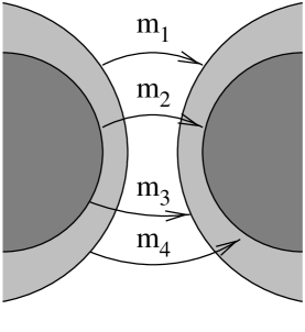
FIG. 3.: One representation of the four operators tunneling quasiparticles between two $\nu=2/5$ edges, each of which contains two branches of edge modes.

As an example of the above, consider tunneling between $\nu=2/5$ states, where each subedge contains two modes (Fig. 3). There is a three-dimensional subspace of neutral operators of the combined system (the four operators indicated in Fig. 3 are linearly dependent), and $D$ boundary conditions on all neutral modes corresponds to lattice duality in a three-dimensional subspace and leading operator dimensions $(2/5,11/10,\ldots)$, while the fixed point preserving the folding symmetry corresponds to duality in a two-dimensional subspace (two neutral modes get $D$) and leading operator dimensions $(2/5,3/5,\ldots)$, which are the dimensions of quasiparticle tunneling operators. The two modes which pass to $D$ boundary conditions can be taken to be ${\bf m}_{1}$ and ${\bf m}_{2}$ in Fig. 3. The possibility of different fixed points suggests that if the folding symmetry is broken, e.g., by having multiple tunneling points, the true strong-coupling point could correspond to the full three-dimensional duality.

It is easy to prove that, with the restriction of folding symmetry, the dual of electron tunneling between the same state $\nu$ is quasiparticle tunneling. The duality takes place in the $n$-dimensional subspace of operators $({\bf m},-{\bf m})$ in our unfolded notation, since only the $n$ even combinations couple to the impurity. In the case of $\nu=1$ to $\nu=2/5$ tunneling discussed above, there is one neutral mode which can be either $N$ or $D$ without altering the value of the conductance. The choice $D$ taken above corresponds to duality in a two-dimensional subspace, while $N$ gives a leading tunneling operator of dimension $1/7$ and transferred charge $2e/7$, which may be realizable if some tunneling operators are tuned to zero. We see that the symmetries of a given tunneling problem help determine which of the $\sigma=\sigma_{hm}$ fixed points is physically appropriate.

IV Conclusions

Our approach has been to study edge tunneling between general quantum Hall states at three increasing levels of sophistication. A simple energy conservation argument gives an upper bound on the conductance of a tunnel junction, and the Kubo formula applied to the $\chi$LL theory of the edge modes indicates that the bound is saturated for Dirichlet boundary conditions on the neutral mode which transfers charge between the edges. The same picture of strong-weak duality previously obtained for the single-mode case also applies to the general case, but with some new features: the duality in the multiple-mode case does not reduce to independent dualities on individual neutral modes of the combined system, but instead is a multidimensional lattice duality. For tunneling between specific filling fractions, there can be several different fixed points with the dissipationless value of conductance corresponding to dualities on different sets of neutral modes; which fixed point is the physical high-voltage limit can be determined from symmetry considerations. In sum, we have shown that the $\chi$LL model applied to hierarchical edges has a consistent and physically reasonable strong-coupling limit with interesting alterations from the exactly solvable single-mode case. The conductance, noise, and operator content at strong coupling can be compared to possible experiments and to the predictions of other theories.

The authors wish to thank E. Fradkin and X.-G. Wen for helpful comments. Support was provided by the Fannie and John Hertz Foundation (J. E. M.), NSF Grant DMR-98-76208 (P. S. and C. C.), and the Alfred P. Sloan Foundation (C. C.).

REFERENCES

- [1] X.-G. Wen, Phys. Rev. B 43, 11025 (1991); Phys. Rev. Lett. 64, 2206 (1990); Adv. in Phys. 44, 405 (1995).
- [2] C. L. Kane, M. P. A. Fisher, and J. Polchinski, Phys. Rev. Lett. 72, 4129 (1994).
- [3] J. E. Moore and X.-G. Wen, Phys. Rev. B 57, 10138 (1998).
- [4] A. V. Shytov, L. S. Levitov, and B. I. Halperin, Phys. Rev. Lett. 80, 141 (1998).
- [5] M. Grayson et al., Phys. Rev. Lett. 80, 1062 (1998).
- [6] A. M. Chang, unpublished.
- [7] D.-H. Lee and X.-G. Wen, cond-mat/9809160; A. Lopez and E. Fradkin, Phys. Rev. B 59, 15323 (1999); S. Conti and G. Vignale, cond-mat/9801318; D. V. Khveshchenko, Solid State Comm. 111, 501 (1999); U. Zülicke and A.H. MacDonald, Phys. Rev. B 60, 1837 (1999); V. Pasquier and D. Serban, cond-mat/9912218.
- [8] P. Fendley, A. W. W. Ludwig, and H. Saleur, Phys. Rev. B 12, 8934 (1995).
- [9] D. B. Chklovskii and B. I. Halperin, Physica E 1, 75 (1997).
- [10] C. Chamon and E. Fradkin, Phys. Rev. B 56, 2012 (1997).
- [11] N. P. Sandler, C. Chamon, and E. Fradkin, Phys. Rev. B 59, 12521 (1999).
- [12] J. E. Moore and X.-G. Wen, unpublished.
- [13] C. L. Kane and M. P. A. Fisher, Phys. Rev. B 46, 15233 (1992).
- [14] C. Nayak et al., Phys. Rev. B 59, 15694 (1999).
- [15] A. Schmid, Phys. Rev. Lett. 51, 1506 (1983).
- [16] J. L. Cardy, Nucl. Phys. B 270, 186 (1986).
- [17] H. Saleur, “Lectures on non-perturbative field theory and quantum impurity problems,” to be published in Les Houches 1998 proceedings, cond-mat/9812110.