A Monte Carlo analysis of the phase transitions in the $2D$, $J_{1}-J_{2}$ XY model

Abstract

We consider the $2D$ $J_{1}-J_{2}$ classical XY model on a square lattice. In the frustrated phase corresponding to $J_{2}>J_{1}/2$, an Ising like order parameter emerges by an “order due to disorder” effect. This leads to a discrete $Z_{2}$ symmetry plus the $U(1)$ global one. Using a powerful algorithm we show that the system undergoes two transitions at different but still very close temperatures, one of Kosterlitz-Thouless (KT) type and another one which does not belong to the expected Ising universality class. A new analysis of the KT transition has been developed in order to avoid the use of the non-universal helicity jump and to allow the computation of the exponents without a precise determination of the critical temperature. Moreover, our huge number of data enables us to exhibit the existence of large finite size effects explaining the dispersed results found in the literature concerning the more studied frustrated $2D$, XY models.

PACS NUMBERS: 05.50.+q, 75.10.Hk, 05.70.Fh, 64.60.Cn, 75.10.-b

I Introduction

The ground state of a large class of two-dimensional classical frustrated XY models have the particularity to exhibit both continuous and discrete $Z_{2}$ degeneracy simultaneously in the ground state. It results the appearance of a new Ising-like order parameter, in addition to the continuous $U(1)$ symmetry. The most famous example exhibiting such behaviors is certainly the fully frustrated XY model (FFXY) which was originally introduced by Villain as a frustrated XY model without disorder [1]. In this model, the $Z_{2}$ symmetry is associated with the two types of chirality ordering. This model is also of great interest because it describes a superconducting array of Josephson junctions under an external transverse magnetic field such that the flux per plaquette is half the quantum flux [2]. For fifteen years, extensive (essentially numerical) works have been carried on the FFXY [3]-[10] and also to some related models like the triangular antiferromagnetic XY model[11], the helical XY model[12], the Coulomb gas system of half integer charges [13, 14]. The interplay between the two transitions can lead a priori to two transitions, namely a Kosterlitz-Thouless one and an Ising one. Nevertheless, the entanglement between the two order parameters considerably complicates the analysis. The nature of the phase diagram is still rather unconclusive and controversial. Three different scenari have been advocated: either the two transitions occur at the same point and eventually merge to give a new universality class [5, 6, 4, 7]; or the two transitions occur at different points and are of Ising and Kosterlitz-Thouless types plus some strong finite size effects [13, 15]; or finally the two transitions are effectively separated but the transition associated to the chiral order parameter is not of Ising type [8, 9, 14]. The most recent numerical studies are in favor of the latter scenario. Nonetheless, without a strong analytical support, the problem is still completely open.

The purpose of the present article is other. We want to clarify the critical behavior of a less studied frustrated XY model: the $2D$, $J_{1}-J_{2}$ XY model on a square lattice which, as will be shown, is in the same universality class as the models quoted above (or more precisely has the same problematic). The Hamiltonian reads

$$H = -J_{1}\sum\limits_{<i,j>}{\bf S}_{i}{\bf S}_{j}+J_{2}\sum\limits_{<<k,l>>}{\bf S}_{k}{\bf S}_{l}$$ (1)

$$= -J_{1}\sum\limits_{<i,j>}\cos(\theta_{i}-\theta_{j})+J_{2}\sum\limits_{<<k,l>>}\cos(\theta_{k}-\theta_{l})~{},$$ (2)

where ${\bf S}_{i}$ are two component classical vectors of unit length, with $J_{1},J_{2}>0$, $<~{}>$ and $<<~{}>>$ indicate respectively the sum over nearest neighbors and next to nearest neighbors. When $2J_{1}>J_{2}$ the ground state is ferromagnetic. It leads to a Kosterlitz-Thouless (KT) transition at the temperature $T_{KT}\approx{\pi(J_{1}-2J_{2})\over 2}$ [16]. This temperature is obtained from the Villain treatment of the Hamiltonian (1) (see ref. [17] for details). However, when $2J_{1}<J_{2}$, the ground state consists of two independent $\sqrt{2}\times\sqrt{2}$ sublattices with AF order. The ground state energy $E_{0}=-2NJ_{2}$ does not depend on $\phi$, an angle parameterizing the relative orientations between both sublattices. This non-trivial degeneracy is lifted by thermal fluctuations and a collinear ordering (corresponding to $\phi=0$ or $\pi$) is selected [18]. The two possible ground states are depicted in Fig. 1. The angle $\phi$ thus plays a role analogous to the chiral order parameter. This selection mechanism is one of the most famous “order due to disorder” effect [18] in a sense that fluctuations brings kind of order by lifting this extra continuous symmetry. The resulting symmetry is therefore $U(1)\times Z_{2}$. Monte-Carlo simulations predict only a low temperature phase with a nematic ordering and a disordered high temperature phase [18, 19]. The critical behavior has, as far as we know, only been partially explored in ref. [19]. Unfortunately the results are very approximate and no definite conclusion on the presence of one or two transitions and either on their universality classes has been given. In this work, we have carried on extensive numerical Monte Carlo simulations on the $J_{1}-J_{2}$ XY model using algorithms which allow us to obtain very accurate and robust results.

We now give the outline of the paper. Section 2 contains a brief summary of analytical results showing the relations between the $J_{1}-J_{2}$ XY model and the Ising-XY model, which is a generic model used to describe the universality class of frustrated XY models with symmetry $Z_{2}\times U(1)$ like the FFXY. In section 3, we present our numerical results and the analysis of some critical exponents. Finally, section 4 is devoted to the discussion of the results and to a brief conclusion. The estimation of statistical and systematic errors has been relegated in the appendices.

II The $J_{1}-J_{2}$ XY and Ising-XY model

In this section, we sum up the main analytical results concerning the $J_{1}-J_{2}$ XY model. We essentially focus on the more interesting frustrated phase corresponding to $2J_{2}>J_{1}$, where the ground state consists of two independent sublattices. Thermal fluctuations select a collinear ordering [18], and we have two kinds of domains represented in Fig. 1. The first step, following Chandra et al. [20], is to perform a gradient expansion of the classical energy (1). The problem is now translated in a new one on a $(2\times 2)$ square lattice, but now with two spins $1$ and $2$ per vertices pointing in the same directions. The new classical action ${\cal A}$ reads

$${\cal A} = -{2J_{2}\over 2T}\sum\limits_{r}\left[(\vec{\nabla}\theta_{1})^{2}+(\vec{\nabla}\theta_{2})^{2}\right.$$ (3)

$$+ \left.2\lambda\cos\phi~{}~{}(\nabla^{x}\theta_{1}\nabla^{x}\theta_{2}-\nabla^{y}\theta_{1}\nabla^{y}\theta_{2})\right]~{},$$ (4)

where we have defined $\lambda={J_{1}\over 2J_{2}}<1$ and introduced the lattice derivatives $\nabla^{x},~{}\nabla^{y}$ [16]. The signature of the $U(1)$ degeneracy lies now in the strong anisotropy between $x$ and $y$ directions. The $\cos\phi$ labels the different possible classical ground states at $T=0$. Notice that, if we do the Gaussian integration over the angular variables, we recover the results of Henley [18], namely

$${\cal A}\sim const-0.32\left({J_{1}\cos\phi\over 2J_{2}}\right)^{2}~{},$$ (5)

proving that a collinear ordering is selected when minimizing the free energy($\cos(\phi)=\pm 1$).

Let us now include the effects of the vortices. The most natural way to include them would be to apply the Villain transformation to all quadratic terms in the action (3). Such a treatment is quite tedious and unappropriated because the vortices variables built with the anisotropic term $(\nabla^{x}\theta_{1}\nabla^{x}\theta_{2}-\nabla^{y}\theta_{1}\nabla^{y}\theta_{2})$ are not well defined due to the strong fluctuations between the two sublattices which tend to decouple in the infrared limit ( see [16] for more details). A simplest way to take into account the coupling between the two sublattices is to replace the anisotropic term in (3) by the local spin waves effect i.e. by $-0.32\lambda^{2}\sum\limits_{r}\cos^{2}(\theta_{1}(r)-\theta_{2}(r))$. This term is just the local version of (5). Such a treatment has already been used by Garel et al. for helimagnets [12] and also by Chandra et al. for the $J_{1}-J_{2}$ Heisenberg model [20]. By applying the Villain transformation to the first two terms in (3) and using

$$\exp\left[h\cos p(\theta_{1}(\vec{r})-\theta_{2}(\vec{r}))\right]= \sum\limits_{S(\vec{r})}\exp\left[ipS(\vec{r})(\theta_{1}(\vec{r})-\theta_{2}(\vec{r}))\right.$$ (7)

$$+\left.\log y_{s}S^{2}(\vec{r})\right],$$

with $p=2$ and $y_{s}=h/2=0.08\lambda^{2}$, we obtain

$${\cal Z}=\sum\limits_{\{n_{1}^{\mu}(r)\}}\sum\limits_{\{n_{2}^{\mu}(r)\}}\sum\limits_{S(r)} \int{\cal D}\theta_{1}{\cal D}\theta_{2}\exp\left(-{J_{2}\over T}\sum\limits_{r}\sum\limits_{i=1,2}\left[(\nabla^{\mu}\theta_{i}(r)-2\pi n_{i}^{\mu}(r))^{2}\right]\right.$$ (8)

$$+ ip\left.\sum\limits_{r}\left[S(r)(\theta_{1}(\vec{r})-\theta_{2}(\vec{r}))+\log y_{s}S^{2}(\vec{r})\right]\right)$$ (9)

The $n_{i}^{\mu}$ ($i=1,2$) are integer link variables living on the two diagonal sublattices. By integrating on angular variables, we easily find

$${\cal A}_{eff} =\sum\limits_{r\neq r^{\prime}}\left[\pi\beta J_{2}M_{1}(r)\log{|r-r^{\prime}|\over a}M_{1}(r^{\prime})+\pi\beta J_{2}M_{2}(r)\log{|r-r^{\prime}|\over a}M_{2}(r^{\prime})\right.$$ (12)

$$-ip(M_{1}(r)+M_{2}(r))\Theta|r-r^{\prime}|S(r^{\prime})+\left.{p^{2}\over 2\pi\beta}S(r)\log{|r-r^{\prime}|\over a}S(r^{\prime})\right]$$

$$+\sum\limits_{r}\left[\log y_{1}~{}(M_{1})^{2}(r)+\log y_{2}~{}(M_{2})^{2}(r)+\log y_{s}~{}S^{2}(r)\right]~{},$$

where we have introduced the vortex variables $M_{i}=\epsilon^{\mu\nu}\nabla^{\mu}n_{i}^{\nu}$ corresponding to vortices on the two sublattices. The fugacities are as usual considered as genuine variables defined initially by $y_{i}^{0}=\exp(-{\pi^{2}\beta J_{2}\over 2})$. The interaction $\Theta$ is defined by $\Theta|r-r^{\prime}|=\arctan({y-y^{\prime}\over x-x^{\prime}})$, and verifies $\partial_{y}\log|r-r^{\prime}|=-\partial_{x}\Theta|r-r^{\prime}|$. This action corresponds to two coupled XY models. Under real space renormalization group transformations, the coupling term is strongly relevant and locks the phase difference in $\theta_{1}(r)=\theta_{2}(r)+k\pi$ with $k=0,1$ [21]. It leads in the strong coupling limit to an effective model whose Hamiltonian has the following form

$$H_{I-XY}=-\sum\limits_{<i,j>}[A(1+\sigma_{i}\sigma_{j})\cos(\theta_{i}-\theta_{j})+C\sigma_{i}\sigma_{j}]~{}.$$ (13)

The value of $A$ and $C$ depend of the initial values of $h=f(J_{1},J_{2})$ and $\beta J_{2}$. This model refereed as the Ising-XY model in the literature has been largely debated. This Ising-XY model is believed to describe the critical behavior of all frustrated XY models quoted in the introduction. The phase diagram has been obtained numerically by Granato et al. [22] and has been reproduced for convenience in Fig. 2. Three different phases can be distinguished: the upper right corner phase correspond to the low temperature ordered phase, the low left corner phase is the high temperature disordered one, and the intermediate one is Ising ordered but XY disordered (namely with free vortices). Above the point $P$, the Ising and XY transitions are well separated and mix under P. The question concerning the transition(s) under $P$ is still under debate. A recent work of S. Lee et al. seems to indicate that the two transitions never merge completely but get closer [15]. Nevertheless the Ising-like magnetization exponent has been found different from $1$ and continuously varying along the line (PT) [22]. We have shown that the $J_{1}-J_{2}$ XY model should be also described by the Ising-XY model and should therefore correspond to a curve crossing the line under P (so with only one or two very close transitions). Since we are not able to provide analytical relations between $(h,J_{2})$ and $(A,C)$, the form of this curve and its intersection with the segment (PT) is unaccessible. Moreover, when varying $J_{2}/J_{1}$, we shall obtain a different intersection point as it was firstly noted in [16]. Nevertheless, it opens the possibility that the critical exponent $\nu$ should vary with the ratio $J_{2}/J_{1}$ as in the analysis of Granato al. [22] or of Lee al. [15]. Similar considerations have been done in the study of a generalized frustrated XY model where an extra-parameter has been added [10]. No clear conclusion concerning the nature of the phase transitions can be therefore drawn at this level. The purpose of the next section is therefore to answer these questions by help of extensive Monte Carlo simulations. Moreover, it can also be regarded as an indirect way of studying the Ising-XY model and other related models.

III Monte Carlo analysis

A Observables

As explained above we can define two order parameters corresponding to the two symmetries $U(1)$ and $Z_{2}$. The first one is the total magnetization $M$ defined by the sum of all spins, the second is the chirality $\kappa$ defined by the sum of all chiralities $\kappa_{i}$ defined on each cell by:

$$\kappa_{i}={1\over 4}\ (S_{i}-S_{k})(S_{j}-S_{l})$$ (14)

where ($i,j,k,l$) are the four corners of one cell with diagonal (i,k) and (j,l). The two ground states depicted in Fig. 1 have $\kappa_{i}=\pm 1$.

We have studied our system in the finite size scaling region where the correlation length is much bigger than the lattice size. The quantities needed for our analysis are defined below. For each temperature we calculate:

$$\chi^{M} = {{N<M^{2}>}\over{k_{B}T}}$$ (15)

$$\chi^{\kappa} = {{N(<\kappa^{2}>-<\kappa>^{2})}\over{k_{B}T}}$$ (16)

$$\chi_{2}^{\kappa} = {{N<\kappa^{2}>}\over{k_{B}T}}$$ (17)

$$V_{1}^{\kappa} = {{<\kappa E>}\over{<\kappa>}}-<E>$$ (18)

$$V_{2}^{\kappa} = {{<\kappa^{2}E>}\over{<\kappa^{2}>}}-<E>$$ (19)

$$V_{2}^{M} = {{<M^{2}E>}\over{<M^{2}>}}-<E>$$ (20)

$$U^{M} = 1-{{<M^{4}>}\over{3<M^{2}>^{2}}}$$ (21)

$$U^{\kappa} = 1-{{<\kappa^{4}>}\over{3<\kappa^{2}>^{2}}}$$ (22)

where $E$ is the energy, $\chi$ is the magnetic susceptibility per site, $V_{1,2}$ are cumulants used to obtain the critical exponent $\nu$, $U$ are the fourth order cumulants, $<...>$ means the thermal average.

B Algorithm

We use in this work the standard Metropolis algorithm. At each site a new random orientation for the spin is chosen. The interaction energy between this spin and its neighbors is then calculated. If lower than the energy of the old state, the new state is accepted, otherwise, it is accepted only with a probability $p$ according to the standard Metropolis algorithm.

However the critical slowing down is important and we improve the speed of the simulation using the local over-relaxation algorithm (OR) [23]. This algorithm consists in choosing the new orientation of the spin such that the energy remains unchanged. For $XY$ spins the only possibility is to take the symmetric of the old spin to the local field (the sum of the neighbors). This algorithm is obviously non ergodic, i.e. all states can not be reached. It must thus be used in combination with the standard Metropolis algorithm (MET). Therefore, at each step (regarded as one unit) we use one MET step and a certain number of steps of over-relaxation ($NOR$) algorithm. The larger $NOR$, the smaller the autocorrelation time (the number of steps between two independent configurations), but then the larger the time needed for each step is. We have thus to choose the best $NOR$ to minimize the real autocorrelation time. This depends on the time needed for each algorithm. In our implementation the Metropolis algorithm is six times larger than the over relaxation algorithm.

In order to calculate the autocorrelation time we follow the procedure explained in appendix A. In table I we present the results of the autocorrelation time $\tau_{\kappa}$ for different $NOR$ at the critical temperature $T_{c}^{\kappa}$ for a lattice size $L=30$ and $J_{2}/J_{1}=0.7$. The second column gives $\tau_{\kappa}$ while the third column gives the real autocorrelation time $\tau_{\kappa}\,(1+NOR/6)$, i.e. the quantity to be minimized. The value $NOR\sim L/5=6$ seems to fit best. We have checked that this ratio does not change significantly for sizes $L=20$ and $L=40$, which is in agreement with the argument of Adler [24] where the best $NOR$ should be proportional to the correlation length, i.e. to the lattice size in the finite size scaling region.

In Fig 3 we have shown in a log-log scale the real chirality autocorrelation time function of the lattice size for $NOR=0$ and $NOR=L/5$. For larger lattice sizes the gain is more than a factor 30 using the over relaxation algorithm. The critical exponent $z$ defined by $\tau\sim L^{z}$ is 2.29(4) without the use of the OR algorithm and is in agreement with the results on the Villain lattice 2.31 [25] but in disagreement with the dynamic approach of Luo et al. [9] who obtained 2.17(4). We note for this last case that an error on $z$ leads to errors on the other exponents.

In the following the simulations have been done using $NOR=L/5$ for each Metropolis algorithm. For each simulation, we use a number $t_{av}$ measurements, made after an updating time $t_{up}$ is carried out for equilibration. For each size, between three and six different initial configurations (ordered or random) have been tested to be sure that our system is not trapped into a metastable state. In table II we present some details of our simulations. We want to stress that the number of Monte Carlo steps used in this work is one order of magnitude larger than previous studies and, combined with a better algorithm, produces a better estimate of the thermodynamic quantities.

Our errors are calculated with the help of the Jackknife procedure [26]. When compiling the different results from previous studies we have noticed that the errors reported are quite often strongly underestimated. Therefore we have presented in the appendix A our method to evaluate the errors coming from the simulation and in particular a simplified method of the Jackknife procedure.

We use in this work the histogram MC technique developed by Ferrenberg and Swendsen [27, 28]. From a simulation done at $T_{0}$, this technique allows to obtain thermodynamic quantities at $T$ close to $T_{0}$.

C Phase diagram

We have performed many simulations in varying the value of $J_{2}/J_{1}$ to obtain the critical temperature $T_{c}$ which is represented in Fig 4. The transition for $J_{2}/J_{1}<0.5$ is a standard Kosterlitz-Thouless transition in agreement with theoretical predictions. For $J_{2}/J_{1}>0.5$ it is difficult to discriminate between the hypothesis of one or two transitions separating the low temperature nematic phase from the high temperature disordered phase. We have therefore decided to focus on the particular value $J_{2}=0.7,J_{1}=1.$ (black circle) in the remainder of this work. It is worth noticing that Fernandez et al. [19] have done their calculation for $J_{2}=J_{1}=1$.

As it was first emphasized in section 2, it is possible that the exponents could vary with the ratio $J_{2}/J_{1}$ [16]. This should be coherent with the picture proposed by Granato et al for the Ising-$XY$ model [22] and by Lee et al. [15]. Nevertheless, the first step is to perform very highly accurate Monte Carlo simulations at some fixed value of $J_{2}/J_{1}$ to show the existence to test the existence of two close transitions, and check that the chiral magnetic exponent $\nu$ is clearly different from $1$.

D $Z_{2}$ symmetry

We concentrate first on the breakdown of the $Z_{2}$ symmetry with the order parameter $\kappa$ defined in (14).

To find the critical temperature $T_{c}$ we record the variation of $U^{\kappa}$ with $T$ for various system sizes in Fig 6 and then locate $T^{\kappa}_{c}$ at the intersection of these curves [29] since the ratio of $U^{\kappa}$ for two different lattice sizes $L$ and $L^{\prime}=bL$ should be 1 at $T^{\kappa}_{c}$, namely

$${{{U^{\kappa}_{bL}}\over{U^{\kappa}_{L}}}}\Bigg{\arrowvert}_{T=T_{c}}=\>1\>.$$ (23)

Due to the presence of residual corrections to finite size scaling, one has actually to extrapolate the results taking the limit (ln$b$)${}^{-1}\rightarrow 0$ in the upper part of the Fig. 8. We observe a strong correction for the small sizes. However for the biggest sizes the fit seems good enough and we can extrapolate $T^{\kappa}_{c}$ as

$$T_{c}^{\kappa}=0.56465(8)\ ,$$ (24)

The estimate for the universal quantity $U^{\kappa}_{*}$ at the critical temperature is

$$U^{\kappa}_{*}=0.6269(7).$$ (25)

This value is far away of the two dimensional Ising value $U_{*}^{Ising}\sim 0.611$, [30] which is a strong indication that the universality class associated to the chirality order parameter is not of Ising type. We will verify this prediction studying now the critical exponents.

At $T=T^{\kappa}_{c}$ the critical exponents can be determined by log–log fits. We obtain $\nu^{\kappa}$ from $V_{1}^{\kappa}$ and $V_{2}^{\kappa}$ (Fig. 9), $\gamma^{\kappa}/\nu^{\kappa}$ from $\chi^{\kappa}$ and $\chi_{2}^{\kappa}$ (Fig. 10), and $\beta^{\kappa}/\nu^{\kappa}$ from $\kappa$ (see Fig. 11). We observe in all these figures a strong correction to a direct power law. It is worth noticing however that $X_{2}^{\kappa}$ shows smaller corrections. Using only the three (four for $X_{2}^{\kappa}$) largest terms we obtain:

$$\nu^{\kappa} = 0.795(20)$$ (26)

$$\gamma^{\kappa}/\nu^{\kappa} = 1.750(10)$$ (27)

$$\beta^{\kappa}/\nu^{\kappa} = 0.127(10)\ .$$ (28)

The uncertainty of $T^{\kappa}_{c}$ is included in the estimation of the errors. The large values in our errors come from the use of only few sizes for our fits. If we had used more, the exponents would change and for example $\nu^{\kappa}$ would grow until 0.91 using all the sizes. The non observation of the corrections in previous studies could explain the very dispersed results obtained in various studies of different frustrated $2D$ XY models (between 0.76 to 0.90). We note that we have used much more statistics (due to one part to a better algorithm, and in other part to longer simulations) than previous works (between one or two order of magnitude more) which enables us to observe the finite size corrections. Moreover, we expect that the critical exponents written above could vary with the ratio $J_{2}/J_{1}$. It makes therefore difficult quantitative comparisons with other studies. Nevertheless, we can safely state that an Ising universality class is excluded. If we try to introduce a correction to calculate the exponents, for example like $V_{1}^{\kappa}=(1+L^{-\omega})L^{1/\nu^{\kappa}}$, we obtain $\omega=1.0(2)$ and values for critical exponents fully compatible with (26-28). We have noticed that the exponents have a tendency to move away from the ferromagnetic Ising values when the size grows and thus seems to exclude a crossover to the ferromagnetic Ising fixed point for larger sizes (unless it occurs at very large and not yet accessible size).

The values given in (26-28) use the properties of the free energy at the critical temperature. But an error on $T^{\kappa}_{c}$ leads to an error on the exponents, it is therefore interesting to find them without the help of $T^{\kappa}_{c}$. This can be done using the whole finite size scaling region and the method given in [31]. It consists to plot, for example, the susceptibility $X^{\kappa}L^{-\gamma^{\kappa}/\nu^{\kappa}}$ as function of $U^{\kappa}$, choosing the exponents as the curves collapse. This fit is stronger than the fit at the critical temperature in so far as it does not depend only on results at $T^{\kappa}_{c}$ but on a large region of temperature. However the errors are a little bit larger. We show in Fig. 12-14 the results for three choices of $\gamma^{\kappa}/\nu^{\kappa}$. Obviously the result $\gamma^{\kappa}/\nu^{\kappa}=1.76$ is the best one. With this method we arrive at $\gamma^{\kappa}/\nu^{\kappa}=1.76(2)$ which is compatible with the result (27) and thus constitutes an indirect check of the critical temperature. We have verified, using cumulants $V_{1}$ and $V_{2}$ and $<\kappa>$, that the results for $\nu^{\kappa}$ and $\beta^{\kappa}/\nu^{\kappa}$ are compatible with (26) and (28).

From the scaling relation

$$\gamma^{\kappa}/\nu^{\kappa}=2-\eta^{\kappa}$$ (29)

we obtain $\eta^{\kappa}=0.25(1)$. The results are summarized in table III.

In conclusion the chirality order parameter does not seem to belong to the standard two dimensional Ising universality class. Such conclusion has already been reached in many studies of frustrated XY models. Nevertheless, due to the fact that the exponents could be $J_{2}/J_{1}$ dependent, we cannot safely compare the results we get for the $J_{1}-J_{2}$ XY model with other frustrated XY models. However we observe that the exponents vary strongly if corrections are not taken into account and we suspect that this is also the case in the other studied models.

If the transition belongs to a new universality class, the use of Binder’s cumulant at the critical temperature $U^{\kappa}_{*}$ could be a new approach to track it. It should be very interesting to test this idea in other systems like the Villain or the triangular models.

E $U(1)$ symmetry

We now focus on the phase transition associated to the $U(1)$ symmetry, i.e. to the $XY$ spins. The usual ferromagnetic XY model undergoes a Kosterlitz-Thouless phase transition driven by the unbounding of vortex-antivortex pairs. The best method to obtain reliable results is to use the jump of the helicity parameter defined by the answer of the system to a twist in one direction. The knowledge of the jump at the critical temperature allows to obtain $T_{c}$ with a good precision [32]. However, in our problem the presence of the chirality order parameter coupled with topological defects leads to a non-universal jump. This fact explains why this transition is usually not explored in Monte-Carlo simulations of frustrated XY models or, when it is, why results are not very accurate. In the following study we will use a method introduced in [33] using Binder’s cumulant to study this transition. It was proved in this article that, contrary to the common belief, the Binder cumulant for ferromagnetic XY systems crosses for different sizes, allowing thus a rough estimate of the critical temperature and especially of the exponent $\eta$ without the precise knowledge of the critical temperature.

We proceed in a way similar as for the Ising order parameter, replacing $\kappa$ by $M$. We record the variation of $U^{M}$ (31) with the temperature for various system sizes in Fig 7. We want to underline the differences between the result of $U^{\kappa}$ (Fig 7) and $U^{M}$ which are plotted with the same scale. $U^{M}$ shows a crossing on a smaller region than $U^{\kappa}$, and at least one order of magnitude less than the standard XY model (see the figure 1 of [33]) We then locate the intersection of these curves and plot the results in the lower part of the Fig. 8.

Let us first consider a power law behavior at $T>Tc$ for this system. In this case we have to consider a linear fit for (ln$b$)${}^{-1}\rightarrow 0$. We observe corrections for the smallest size $L=20$ but the others seem to converge to the temperature

$$T_{c}^{M}=0.56271(5)\ .$$ (30)

Secondly we consider the behavior to be exponential as in the standard $XY$ model. In this case figure 2 of [33] shows that a linear fit could be wrong and that a ”crossover” to a different critical temperature could be observed for bigger $b$, i.e. greater sizes. However contrary to the ferromagnetic XY model, the region of crossing is so small and the different linear fits tend only to one critical temperature. Therefore we think that the linear fit works well enough. Moreover in the following we will show strong arguments in favor of the temperature (30).

With the help of the critical temperature we have found an estimate of $U^{M}$ at $T_{c}^{M}$ fitting the value with a law $U^{M}=U^{M}_{*}+aL^{-\theta}$. We obtain

$$U^{M}_{*}=0.638(5)\ .$$ (31)

By log–log fit we calculate some exponents. The exponent $\eta$ could be obtained by a fit with $X_{2}^{M}$ shown in Fig 10. We obtain here

$$2-\eta^{M} = 1.657(5)$$ (32)

$$\eta^{M} = 0.345(5)$$ (33)

The fit has been done discarding the two smallest sizes ($L=20$ and $L=40$) which show small corrections. This value is different from the standard XY case where $\eta=0.25$. Notice also that it is in contradiction with the result of Monte Carlo simulations in the high temperature region obtained by José et al. [6] for the FFXY (which is believed to be in the same universality class as our model) where $\eta\sim 0.20$ was found. To our knowledge, it seems one of the first times this exponent is calculated using finite size scaling. From a theoretical point of view the $KT$ transition has an exponential behavior, i.e. a correlation length of the form $\xi\sim\exp[B_{0}\,(T-T_{c})^{-\nu}]$, however a power law behavior like ($\xi\sim(T-T_{c})^{-\nu}$) can not be excluded numerically. In the latter case the critical exponent $\nu$ can be calculated with the cumulant $V_{2}^{M}$ (20). We have obtained $\nu^{M}=0.92(3)$. With the finite size scaling method we were not able to compute the exponent $\nu$ in the case of an exponential behavior.

As for the Ising order parameter, the calculation of the exponents have been done at the critical temperature but an error on $T_{c}^{M}$ leads to errors on the exponents, it is thus interesting to find them without the help of $T^{M}_{c}$. This can be done using the same method as described before. We have shown in [33] that this method is accurate enough in order to obtain $\eta$ whatever the type of the behavior is (power law or exponential). In Fig. 15-17 we show our results for three values of $\eta^{M}$. Obviously the value $\eta^{M}=0.33$ is the best and we are able to obtain:

$$\eta^{M}=0.33(2)$$ (34)

which is compatible with (33). Moreover this result is a strong indication that our choice of the critical temperature is correct. Indeed another choice leads to other non-compatible exponents. For example, had we chosen $T_{c}^{M}=T_{c}^{\kappa}=0.56465$ we would obtain $\eta^{M}(T=T_{c})=0.47$ which is incompatible with (34).

To sum up, we have computed for the first time the critical exponent $\eta^{M}=0.345(5)$ for the Kosterlitz-Thouless transition using the finite size scaling region in Monte Carlo simulations. We have given strong arguments that, in our range of sizes, the critical temperature for this transition is less than the critical temperature corresponding to the Ising-like transition ($T_{c}^{M}<T_{c}^{\kappa}$). Note that this is in agreement with the phase diagram of the Ising-XY model (Fig 2), where if the two transitions never merge, we have $T_{KT}<T_{I}$ (see also ref. [15]). We cannot exclude, contrary to the ferromagnetic XY model, a power law behavior at $T>T_{c}^{M}$ which should be characterized besides the exponent $\eta^{M}$, by $\nu^{M}\sim 0.92$ and $U^{M}_{*}\sim 0.638$.

IV Conclusion

In this paper we have investigated the critical behavior of the $2D$, $J_{1}-J_{2}$ XY model on the square lattice. We have first theoretically argued that this model should be in the same universality class as the Ising-XY model for $2J_{2}>J_{1}$. We have then carried on extensive Monte Carlo simulations for the particular ratio $J_{2}/J_{1}=0.7$. Our main conclusion is that this system undergoes two distinct and separate transitions. The first one is of Kosterlitz-Thouless type with an exponent $\eta=0.345(5)$ different to the ferromagnetic case, whereas the second one (associated to the chirality order parameter) seems to be in a non-Ising universality class. The temperatures of transitions and the values of the critical exponents are summarized in table III. It is worth mentioning that the estimate of the exponents can be obtained without the help of a precise determination of the critical temperatures. The values of the critical exponents associated to the Ising symmetry are consistent with those obtained in various recent works for different frustrated XY models [4, 6, 8, 9, 15]. Nevertheless, our analysis has been done at $J_{2}/J_{1}=0.7$. We expect that the exponents we obtained could vary with the ratio $J_{2}/J_{1}$ which makes accurate comparisons difficult. Consequently, numerically speaking, we cannot safely state that the $J_{1}-J_{2}$ XY model is in the same universality class as other models quoted above.

The fact that two transitions exist at two different temperatures and that the critical exponents of the chiral order parameter transition is not of Ising type seems puzzling. How could we reconciliate them ? One first idea, is to use an argument by Olsson [13] which explains these strong deviations from the Ising universality class by a large screening length (due to vortices) which prevents observing the expected Ising behavior. In our case, we would therefore expect for large sizes, a crossover to such behavior, i.e. for example, $\nu$ grows to reach the value 1 for an infinite size. However no sign of this crossover has appeared for our largest sizes ($L=150$). Obviously, such a crossover could not be excluded for much larger size ($L\sim 1000$) but seems not very plausible. Two more plausible interpretations can be a priori formulated. One, due to Granato et al. [7] consists in invoking a new universality class for the chiral order parameter. The idea of the $3-$state Potts model universality class has for example been recently advocated in [8]. Another one is due to Knops et al. [4]. These authors have introduced a possible instable fixed point on the critical line PT of the phase diagram of the Ising-XY model (see Fig. 2) which is able to induce strong cross over phenomena in the infrared limit. This conjecture has the advantage to explain the whole set of dispersed results found in the literature. Notably, it would explain the continuous variation of exponents found by Granato et al. in the Ising-XY model [22] but also the the $J_{2}/J_{1}$ dependence of critical exponents in the $J_{1}-J_{2}$ XY model under consideration here. To answer these questions, very high precision Monte-Carlo simulations for large size systems could bring some answers to this problem. Moreover new analytical developments are deeply needed.

V Acknowledgments

This work was supported by the Alexander von Humboldt Foundation and the EC TMR Program Integrability, non-perturbative effects and symmetry in Quantum Field Theories, grant FMRX-CT96-0012

$NOR$	$\tau_{\kappa}$	$\tau_{\kappa}\,(1+NOR/6)$
0	256(9)	256(9)
2	18.9(4)	25.1(5)
3	14.5(2)	21.7(3)
4	12.3(2)	20.5(3)
5	11.2(1)	20.5(2)
6	10.2(2)	20.3(3)
7	9.5(2)	20.5(3)
10	8.4(1)	22.4(2)
15	7.50(4)	26.2(1)

TABLE I.: Autocorrelation times for the chirality for $L=30$ in function of the number of over-relaxation steps $NOR$.

$L$	$t_{up}$	$t_{av}$	$\tau_{\kappa}$	$t_{av}/\tau_{\kappa}$
20	$5.10^{5}$	$20.10^{6}$	7.95(13)	$2.5\,10^{6}$
40	$5.10^{5}$	$15.10^{6}$	13.19(6)	$1\,10^{6}$
60	$7.10^{5}$	$18.10^{6}$	19.17(17)	$9\,10^{5}$
80	$8.10^{5}$	$18.10^{6}$	25.58(33)	$7\,10^{5}$
100	$1.10^{6}$	$16.10^{6}$	31.66(50)	$5\,10^{5}$
120	$2.10^{6}$	$20.10^{6}$	40.6(10)	$5\,10^{5}$
150	$3.10^{6}$	$32.10^{6}$	50.9(15)	$6\,10^{5}$

TABLE II.: Number of Monte Carlo steps to thermalize $T_{up}$ and to average $T_{av}$ as function of the size of the lattice $L$. $\tau_{\kappa}$ are calculated with shorter MC runs. The last column gives the number of ”independent” measures which are, at least, one or two orders greater than previous studies.

symmetry	$T_{c}$	$U_{*}$	$\nu$	$\gamma/\nu$	$\eta$	$\beta/\nu$
$Z_{2}$	0.56465(8)	0.6269(7)	0.795(20)	1.750(10)	0.250(10)1	0.127(10)
$U(1)$	0.56271(5)	0.638(5)	0.92(3)2		0.345(5)

TABLE III.: Summary of our results for the Ising symmetry ($Z_{2}$) and the $XY$ symmetry $U(1)$. ¹calculated using $2-\eta=\gamma/\nu$. ²for a power law behavior.

A Calculation of errors

We describe here our procedure to calculate statistical errors for the different quantities. The first stage is to find the number of independent steps in our Monte Carlo. Indeed the Monte Carlo is a Markov process and therefore two consecutive steps are correlated.

1 Autocorrelation time

We define the autocorrelation function:

$$\rho(t)={<A(0)A(t)>-<A(t)>^{2}\over<A(t)^{2}>-<A(t)>^{2}},$$ (A1)

where $A(t)$ is a thermodynamic quantity ($\kappa$, $\chi^{M}$, $\chi^{\kappa}$ …). An example is shown in figure 5 for the chirality $\kappa$ at the temperature $T=T_{c}^{\kappa}$ and for a lattice size $L=20$. $N_{MC}=50$ millions steps of Metropolis algorithm are used after discarding 1 millions steps to thermalize the system. We calculate the autocorrelation time following the procedure of [34] by $\tau=\sum_{t=0}^{t_{f}}\rho(t)$ where $t_{f}$ is calculated in a self consistent way as $\rho(t)<0.01$ which corresponds to $t_{f}\sim 5\tau$. In this case the value we get is systematically underestimated for less than $1$ percent. It is important to stop the summation because the variance of $\tau$ is of the order of the number of summation ($t_{f}$) and thus the error proportional to $\sqrt{t_{f}}$. Madras and Sokal [34] have proposed an estimation of the error:

$$\Delta\tau \sim \sqrt{2(2\,t_{f}+1)\tau^{2}/N_{MC}}\,.$$ (A2)

However this formula seems to underestimate the result. Indeed we calculate $\tau(\Delta\tau)$ function of the number of MC steps. We obtain 104(5), 112(2) and 116.2(8) for one, ten and fifty millions respectively. Obviously the errors are underestimated ($104+5<116.2-0.8$). Therefore, in order to compute the errors for $\tau$ we make several simulations for different initial configurations and use the results as independent quantities to calculate the average and estimate the error.

2 Statistical Errors

The second step after having computed the autocorrelation time $\tau$, is to calculate the error on each quantities. As they depend only on a single average like the chirality or the susceptibility $\chi^{K}_{2}$ (17), the result is straightforward [35]:

$$(\Delta<\kappa>)^{2} = (<\kappa^{2}>-<\kappa>^{2}){(1+2\,\tau/\tau_{s})\over N_{MC}/\tau_{s}},$$ (A3)

$$(\Delta\chi_{2})^{2} = (<\kappa^{4}>-<\kappa^{2}>^{2}){(1+2\,\tau/\tau_{s})\over N_{MC}/\tau_{s}}{N\over k_{B}T},$$ (A4)

where $N_{MC}$ is the number of Monte Carlo steps to average, $\tau_{s}$ the number of steps between two measurements and $N$ the number of lattice sites. Choosing $\tau_{s}=1$ we obtain $(1+2\,\tau)/N_{MC}\sim 2\,\tau/N_{MC}$ for large $\tau$ while choosing $\tau_{s}=\tau$ we get $3\,\tau/N_{MC}$ which gives larger errors.

Problems arise when quantities are a combination of different averages, for example the chirality $\chi^{\kappa}$ (16). We could try to treat $<\kappa>$ and $<\kappa^{2}>$ as independent quantities and estimate the error by the sum of the errors of the two quantities. However the result will be overestimated due to the correlation between the two elements of the sum. To solve this problem we can use, for example, the Jackknife procedure. We do not review this method here but just present the essential points we need (for a more complete review see [26]).

In order to avoid being too abstract, we show how this method works for the susceptibility of the chirality (16). For clarity we choose $\tau_{s}=1$. The application for different $\tau_{s}$ is then straightforward. We have to define

$$\bar{\kappa}_{t} = {N_{MC}\,<\kappa>-\kappa_{t}\over N_{MC}-1}$$ (A5)

$$\bar{\kappa^{2}}_{t} = {N_{MC}\,<\kappa^{2}>-\kappa^{2}_{t}\over N_{MC}-1}$$ (A6)

$$\bar{\chi}_{t} = (\bar{\kappa^{2}}_{t}-\bar{\kappa}_{t}^{2}){N\over k_{B}T}$$ (A7)

where $t$ designs the MC step and $N_{MC}$ the total number of MC steps. Our estimate for the susceptibility and the error will be given by:

$$\chi \sim {1\over N_{MC}}\sum_{t=1}^{N_{MC}}\bar{\chi}_{t}$$ (A8)

$$\Delta\chi^{2} \sim {N_{MC}-1\over N_{MC}}\sum_{t=1}^{N_{MC}}(\bar{\chi}_{t}-\chi)^{2}*(1+2\,\tau)$$ (A9)

If we save the chirality at each MC step the formulas are not difficult to apply. However we need a large hard disc to store the data. For example if we wanted to save the 32 millions steps for the simulation of the size $L=150$ we would then need 72 bytes for each step to save the energy, the magnetization and the chirality, which implies more than two giga bytes. To avoid this problem, we could only save the data every $\tau_{s}=\tau$ but then the size of the file would still be more than ten millions of bytes. Moreover we would lose informations and therefore errors would be greater. We propose now a way which allows to obtain a good estimate without the problem of large storage and with minor changes in the program.

We use a development for large $n=N_{MC}/(1+2\,\tau)$ (which is always the case in MC), choosing $\tau_{s}=1$. In this case the formula (A8-A9) becomes, keeping only the dominant term:

$$\chi \sim (<\kappa^{2}>-<\kappa>^{2}){N\over k_{B}T}$$ (A10)

$$\Delta\chi^{2} \sim {(1+2\,\tau)\over N_{MC}}{[}<\kappa^{4}>-<\kappa^{2}>^{2}+4<\kappa>^{2}(<\kappa^{2}>-<\kappa>^{2})$$ (A12)

$$-4<\kappa>(<\kappa^{3}>-<\kappa^{2}><\kappa>){]}({N\over k_{B}T})^{2}$$

The chirality conserves its initial form while the error is the sum of the two errors (of $<\kappa^{2}>$ and $<\kappa>^{2}$) subtracted by the third term which representing the correlation between them. We note that this procedure induces a small change in the program: we have only to save in the histogram $<\kappa^{3}>$ plus the values of $<\kappa>$ and $<\kappa^{2}>$. To test our formula we have computed the susceptibility associated to the chirality (16) and its errors calculated by three ways. We perform the simulation with a lattice size $L=20$ with 4 steps of over relaxation algorithm between each Monte Carlo, for one million steps. In this case the autocorrelation time is about 8 (see table II). The first method consists in saving at each step the energy, the magnetization and the chirality, the second in saving the data only at each $\tau$ steps, while the third in using the approximate formula (A12). We obtain, respectively: $\chi^{\kappa}=$ 11.22(8), 11.23(10), 11.22(8). The three methods give compatible results but the third one gives the best estimate with the smallest size of storage (some hundred thousands bytes).

We give hereafter the results of our calculation for the binder parameters (21-22) and the cumulant $V_{1}$ and $V_{2}$ (18-19):

$$\Delta{U}^{2} \sim {(1+2\,\tau)\over N_{MC}}{[}4<\kappa^{4}>^{3}-4<\kappa^{2}><\kappa^{4}><\kappa^{6}>+8<\kappa^{2}>^{2}<\kappa^{8}>$$ (A14)

$$-<\kappa^{2}>^{2}<\kappa^{4}>^{2}{]}$$

$$\Delta{V_{1}}^{2} \sim {(1+2\,\tau)\over N_{MC}}{[}{<\kappa E>^{2}\over<\kappa>^{2}}({<\kappa^{2}E^{2}>\over<\kappa E>^{2}}-2{<\kappa^{2}E>\over<\kappa E><\kappa>}+{<\kappa^{2}>\over<\kappa>^{2}})$$ (A17)

$$+<E^{2}>-<E>^{2}$$

$$-2{<\kappa E>\over<\kappa>}({<\kappa E^{2}>\over<\kappa E>}-{<\kappa E>\over<\kappa>}){]}$$

$$\Delta{V_{2}} = \Delta{V_{1}}\ substituing\ \kappa\ by\ \kappa^{2}$$ (A18)

3 Systematic Errors

In addition to statistical errors, we have to take care of systematic errors. There are essentially of two kinds: one due to the correlation between the random number and one due to the use of the histogram technic.

The first one appears when we use a bad random generator. In this case the period of the random numbers could be very small and could thus introduce correlations between data. One example is the linear congruential generator used by many physicist for Monte Carlo simulations! For certain choices of the initial parameter, the period could be very small (less than 2000) and therefore could induce systematic errors. We use in this work a random generator with a period of more than 100 millions found in Numerical Recipes (ran1) [36].

A second source of systematic error comes from the histogram technic and the difference between the temperature of simulation and the temperature where the quantities are computed [37, 38]. In our simulation this difference is kept less than 0.005 in order to minimize this effect.

FIGURE CAPTIONS

Fig. 1: Ground state of the $J_{1}-J_{2}$ XY model for $2J_{2}>J_{1}$

Fig. 2: Phase diagram of the Ising-XY model. Solid and dotted lines indicate continuous and first-order transitions respectively.

Fig. 3: Real autocorrelation time for the standard Metropolis algorithm (circle) and in combination with the over-relaxation algorithm (square).

Fig. 4: Phase diagram for the $J_{1}-J_{2}$ model. For $2J_{2}<J_{1}$ we find the normal Kosterlitz-Thouless transition. Lines are just guides for the eyes. Our study is done for $J_{2}/J_{1}=0.7$ (black circle).

Fig. 5: Autocorrelation $\rho(t)$ for the chirality $\kappa$ at $T=T_{c}^{\kappa}$. The lattice size is $L=20$ and the number of MC is $N_{MC}=50$ millions. The estimated $\tau=116(2)$ is shown by an arrow.

Fig. 6: Binder’s parameter $U^{\kappa}$ for the Ising order parameter function of the temperature for various sizes $L$. The arrow shows the temperature of simulation $T_{s}=0.565$.

Fig. 7: Binder’s parameter $U^{M}$ for the $U(1)$ order parameter function of the temperature for various sizes $L$. The arrow shows the temperature of simulation $T_{s}=0.565$. the scales is similar to those of Fig. 6

Fig. 8: Crossing $T$ plotted vs inverse logarithm of the scale factor $b=L^{\prime}/L$. The upper part of the figure corresponds to $U^{\kappa}$ while the lower part to $U^{M}$. In the last case the size $L=60$ is not shown for clarity. We obtain $T_{c}^{\kappa}=0.56465(8)$ and $T_{c}^{M}=0.56271(5)$ with a linear fit (see text for comments).

Fig. 9: Values of $V_{1}^{\kappa}$ and $V_{2}^{\kappa}$ function of $L$ in a log–log scale at $T_{c}^{\kappa}$. The value of the slopes gives $1/\nu^{\kappa}$. We observe strong corrections for small sizes. Only the three largest sizes are used for the fits. When not shown, the estimated statistical errors are smaller than the symbol.

Fig. 10: Values of $\chi^{\kappa}$ and $\chi_{2}^{\kappa}$ function of $L$ in a log–log scale at $T_{c}^{\kappa}$ and $\chi_{2}^{M}$ at $T_{c}^{M}$. The value of the slopes gives $\gamma/\nu=2-\eta$. We observe strong corrections for the small sizes for $\chi^{\kappa}$. Only the three largest sizes are used for the fit for $\chi^{\kappa}$ while only the smallest sizes $L=20$ and $L=40$ are discarded for the fits for $\chi_{2}^{\kappa}$ and $\chi_{2}^{M}$. When not shown, the estimated statistical errors are smaller than the symbol.

Fig. 11: Values of $<\kappa>$ as function of $L$ in a log–log scale at $T_{c}^{\kappa}$. The value of the slopes gives $\beta^{\kappa}/\nu^{\kappa}$. We observe strong corrections for the small sizes. Only the three largest sizes are used for the fits. When not shown, the estimated statistical errors are smaller than the symbol.

Fig. 12: $\chi^{\kappa}L^{-\gamma^{\kappa}/\nu^{\kappa}}$ function of $U^{\kappa}$ with $\gamma^{\kappa}/\nu^{\kappa}=1.79$ for the sizes $L=60,~{}80,~{}100,~{}120$ and 150. The curves do not collapse in one curve.

Fig. 13: $\chi^{\kappa}L^{-\gamma^{\kappa}/\nu^{\kappa}}$ as function of $U^{\kappa}$ with $\gamma^{\kappa}/\nu^{\kappa}=1.76$ for the sizes $L=60,~{}80,~{}100,~{}120$ and 150. The curves collapse in one curve.

Fig. 14: $\chi^{\kappa}L^{-\gamma^{\kappa}/\nu^{\kappa}}$ function of $U^{\kappa}$ with $\gamma^{\kappa}/\nu^{\kappa}=1.73$ for the sizes $L=60,~{}80,~{}100,~{}120$ and 150. The curves do not collapse in one curve.

Fig. 15: $\chi^{M}L^{2-\eta^{M}}$ function of $U^{M}$ with $\eta^{M}=0.31$ for the sizes $L=60,~{}80,~{}100,~{}120$ and 150. The curves do not collapse in one curve.

Fig. 16: $\chi^{M}L^{2-\eta^{M}}$ function of $U^{M}$ with $\eta^{M}=0.33$ for the sizes $L=60,~{}80,~{}100,~{}120$ and 150. The curves collapse in one curve.

Fig. 17: $\chi^{M}L^{2-\eta^{M}}$ function of $U^{M}$ with $\eta^{M}=0.35$ for the sizes $L=60,~{}80,~{}100,~{}120$ and 150. The curves do not collapse in one curve.

FIG. 1.:

FIG. 2.:

FIG. 3.:

FIG. 4.:

FIG. 5.:

FIG. 6.:

FIG. 7.:

FIG. 8.:

FIG. 9.:

FIG. 10.:

FIG. 11.:

FIG. 12.:

FIG. 13.:

FIG. 14.:

FIG. 15.:

FIG. 16.:

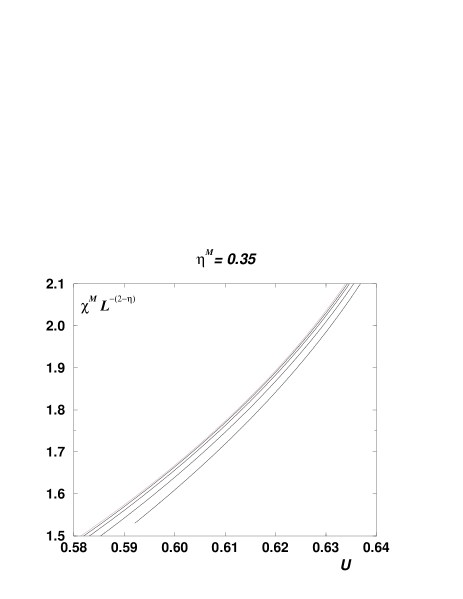
FIG. 17.:

REFERENCES

- [1] J. Villain, J. Phys. C 10, 1717 (1977); ibid 4793 (19977).
- [2] S. Teitel and C. Jayaprakash, Phys. Rev. B 27, 598 (1983); Phys. Rev. Lett. 51, 199 (1983); E. Granato, J. M. Kosterlitz and M. P. Nightingale, Physica B 222, 266 (1996), and references therein.
- [3] B. Berge, H. T. Diep, A. Ghazali and P. Lallemand, Phys. Rev. B 34, 3177 (1986).
- [4] J. M. Thijssen and H. J. F. Knops, Phys. Rev. B 37, 7738 (1988); Y. M. M. Knops, B. Nienhuis, H. J. F. Knops and W. J. Blöte, Phys. Rev. B 50, 1061 (1994).
- [5] J. Lee, J. M. Kosterlitz and E. Granato, Phys. Rev. B 43, 11531 (1991);
- [6] G. Ramirez-Santiago and J.V. José, Phys. Rev. B 49, 9567 (1994); J.V. José and G. Ramirez-Santiago, Phys. Rev. Lett. 77, 4849 (1996).
- [7] E. Granato and M. P. Nightingale, Phys. Rev. B 48, 7438 (1993).
- [8] S. Lee and K.-C. Lee, Phys. Rev. B 49, 15184 (1994).
- [9] H. J. Luo, L. Schuelke and B. Zheng, Phys. Rev. Lett. 81 (1998) 180.
- [10] M. Benakli and E. Granato, Phys. Rev. B 55, 8361 (1997).
-
[11]
D. H. Lee, J. D. Joannopoulos and J. W. Negele,
Phys. Rev. Lett. 52, 433 (1984); Phys. Rev. B 33, 450 (1986);
W. M. Saslow, M. Gabay and W. M. Wang, Phys. Rev. Lett. 68, 3627, (1992). -
[12]
T. Garel and S. Doniach, J. Phys. C 13, L887 (1980);
N. Parga and J. E. Himbergen, Solid. State. Commun. 35, 607 (1980). - [13] P. Olsson, Phys. Rev. Lett. 75, 2758 (1995); Phys. Rev. B 55, 3585 (1997).
- [14] J. R. Lee, Phys. Rev. B 49, 3317, (1994).
- [15] S. Lee, K.-C. Lee and J. M. Kosterlitz, Phys. Rev. B 56, 340 (1997).
- [16] P. Simon, Euro. Phys. lett. 39, 129 (1997).
- [17] P. Simon, J.Phys. A30, 2653 (1997).
- [18] C. L. Henley, Phys. Rev. Lett. 62, 2056 (1989); J. Appl. Phys. 61, 3962 (1987).
- [19] J. F. F. Fernandez, M. Puma and R. F. Angulo, Phys. Rev. B44, 10057 (1991).
- [20] P. Chandra, P. Coleman and A. I. Larkin, Phys. Rev. Lett. 64, 88 (1990).
- [21] M. Yosefin and E. Domany, Phys. Rev. B 32, 1778 (1985); E. Granato, J. M. Kosterlitz, Phys. Rev. B 33, 4767 (1985).
- [22] E. Granato, J. M. Kosterlitz, J. Lee and M. P. Nightingale, Phys. Rev. Lett. 66, 1090 (1991); J. Lee, E. Granato and J. M. Kosterlitz, Phys. Rev. B 44, 4819 (1991); M. P. Nightingale, E. Granato and J. M. Kosterlitz, Phys. Rev. B 52, 7402 (1995).
- [23] M. Creutz, Phys. Rev. D 36, 515 (1987)
- [24] S.L. Adler, Phys. Rev. D 23, 2901 (1981), J. Apostolakis, C.F. Baillie and G.C. Fox, Phys. Rev. D 43, 2687 (1991)
- [25] S. Groe Pawig and K. Pinn, cond-mat/9807137
- [26] B. Efron, The Jackknife, The Bootstrap and other Resampling Plans (SIAM, Philadelphia, PA, 1982)
- [27] A. M. Ferrenberg and R. H. Swendsen, Phys. Rev. Let. 61, 2635 (1988)
- [28] A. M. Ferrenberg and R. H. Swendsen, Phys. Rev. Let. 63, 1195 (1989)
- [29] K. Binder, Z. Phys. B 43, 119 (1981)
- [30] G. Kamienarz and H.W.J. Blöte, J. Phys. A 26 (1993) 201
- [31] D. Loison, Physica A 271, 157 (1999)
- [32] P. Olson, Phys. Rev. B 52, 4527 (1995)
- [33] D. Loison, J. Phys.: Condensed Matter, 11, L401 (1999).
- [34] N. Madras and A.D. Sokal, J. Stat. Phys. 50, 109 (1988) Appendix C
- [35] H. Müller-Krumbhaar and K. Binder, J. Stat. Phys. 8, 1 (1973)
- [36] Numerical Recipes in Fortran, second edition, Cambridge University Press, 1992 (chap. 7).
- [37] A. M. Ferrenberg, D.P. Landau and R.H. Swensen, Phys. Rev. E 51, 5092 (1995)
- [38] M.E.J. Newman and R.G. Palmer, cond-mat/9804306