Instability and Fluctuations of Flux Lines with Point Impurities
in a Parallel Current

Abstract

A parallel current can destabilize a single flux line (FL), or an array of FLs. We consider the effects of pinning by point impurities on this instability. The presence of impurities destroys the long-range order of a flux lattice, leading to the so called Bragg glass (BrG) phase. We first show that the long-range topological order of the BrG is also destroyed by a parallel current. Nonetheless, some degree of short-range order should remain , whose destruction by thermal and impurity fluctuations, as well as the current, is studied here. To this end, we employ a cage model for a single FL in the presence o f impurities and current, and study it analytically (by replica variational methods), and numerically (using a transfer matrix technique). The results are in good agreement, and in conjunction with a Lindemann criterion, provide the boundary in the magnetic field–temperature plane for destruction of short-range order. In all cases, we find that the addition of impurities or current (singly or in combination) leads to further increase in equilibrium FL fluctuations. Thus pinning to point impurities does not stabilize FLs in a parallel current $j_{z}$, although the onset of this instability is much delayed due to large potential barriers that diverge as $j_{z}^{-\mu}$.

I Introduction and Summary

There is currently much effort devoted to understanding the nature of vortex phases in high temperature superconductors [1]. The flux lines (FLs) in a clean material prefer to sit on the sites of a triangular lattice forming an Abrikosov solid for fields $H>H_{c_{1}}$. However, this mean field phase diagram is modified by the combined effects of thermal fluctuations and various types of disorder, such as oxygen vacancies, columnar defects, or twin boundaries. Understanding the precise nature of these new phases is very important for the determination of the transport properties of these materials. In this paper, we focus on the combined effects of point-like disorder, such as oxygen vacancies, and a parallel current. (There are many studies that consider other types of disorder [2, 3]).

It is known that pinning to even a small amount of random impurities is sufficient to destroy the long-range translational order of the Abrikosov lattice[4]. If randomness is strong, the underlying order is destroyed at every scale, but for weak enough randomness, some order is expected to survive at short distances. Indeed, it has been suggested that there may exist a stable, dislocation-free Bragg Glass (BrG) phase at low magnetic fields and temperatures in the presence of weak point impurities [5, 6]. It is important, both for technical applications of high $T_{c}$ materials and from a theoretical point of view, to understand the stability of this new phase with respect to an external current. For example, one may wish to control the melting transition of the BrG phase by some external parameter such as current. The case of a current perpendicular to the vortex lines was studied in Ref. [7], where it was shown that the driven lattice may still maintain a topologically ordered moving BrG phase. Here, we study the case in which current is applied parallel to the FLs. The instability of the proposed equations for the BrG suggests that the long-range topological order of this phase is most likely destroyed by a parallel current. Using a Lindemann criterion and a cage model, we then discuss the destruction of any remnant short range order. This is in the same spirit as a recent calculation[10], in which we used a Langevin equation to examine the dynamics and fluctuations of a FL in the presence of an alternating parallel current. The basic idea is that even in the absence of true long-range order due to current or impurities, there remains a great deal of translational order in the vortex system at short scales. A “phase diagram” is then constructed to indicate the apparent limits of this “ordered” region.

The response of FLs to a parallel current $j_{z}$ was studied extensively even prior to the high-$T_{c}$ era [8]. While, a straight FL is stable in the presence of $j_{z}$, any fluctuation of the line causes helical instabilities at long wavelengths [8]. A lattice of FLs is similarly unstable in the presence of an infinitesimal $j_{z}$, if it penetrates the whole sample. As shown by Brandt [9], for a finite penetration depth of current, a finite $j_{z}\sim{\varepsilon}^{{1}/{4}}$, is needed to cause instability, where $\varepsilon$ is related to the shear modules $c_{66}$. Brandt has suggested [8] that FLs can also be stabilized for infinitesimal $j_{z}$ (which decays exponentially into the sample) due to pinning by disorder. However, this study predates the introduction of the BrG phase, which is more ordered than a flux liquid. We may thus ask if the BrG phase is stable with respect to $j_{z}$? More generally, what is the behavior of the flux line in response to the current $j_{z}$ when point impurities are present? Since, the melting of the BrG phase is thought to be first order, the possibility of diverging longitudinal and perpendicular penetration depths of the current at the transition point is excluded. Nonetheless, we shall assume a current $j_{z}$ which uniformly penetrates the whole sample, and calculate the mean-squared fluctuations of the FL based on this assumption [11, 10]. This quantity is then used to examine the extent of short-range order, and to construct an apparent “phase diagram” in the magnetic field–temperature ($B-T$) plane.

Two models used for the study of FLs with disorder are introduced in Sec. II. The first model describes the elastic behavior of the vortex lattice in the presence of impurities, and is appropriate for the study of its long-wavelength fluctuations. The true long-range order of the lattice is destroyed by such fluctuations, and possibly replaced by the weaker topological order of the proposed Bragg glass[5]. The second model considers a single FL confined by a harmonic cage potential that represents interactions with the other FLs. This model provides an approximate measure of the extent of short-range fluctuations, and in conjunction with a Lindemann criterion can be used to construct a phase diagram[6]. The addition of current to these models is straightforward.

In Sec. III replica variational methods are used to estimate FL fluctuations in the presence of impurities and current. The BrG phase is described by a variational ansatz that breaks full replica symmetry. We propose a natural extension of this solution in the presence of current. This solution, however, has unbounded fluctuations and suffers from the same long-wavelength instabilities as the uniform lattice. We interpret this as a signal of the destruction of BrG order by the current. (Naturally, we cannot rule out other potential variational solutions with other forms of remnant long-range order.) However, it is quite likely that some degree of short-range translational order survives for weak currents and impurities. Using the cage model, we then estimate the fluctuations of a single FL. To this end, we generalize the replica variational ansatz proposed by Goldschmidt[12] to include a current. The mean-squared fluctuations of the FL are found to grow with increasing current and/or impurities. Consequently, in the absence of the cage potential, a single FL is unstable in the presence of an infinitesimal current, and is not stabilized by the impurities alone.

We test the predictions of the replica calculations (for the single FL in a cage) using a transfer matrix method which is introduced in Sec. IV. For a given realization of randomness, this method provides numerically exact results for the extent of fluctuations of a discretized FL in a cage potential. While it is difficult to provide an exact correspondence with the corresponding continuum limit, the results are qualitatively in agreement with those of the replica variational ansatz. In particular, we again find that both impurities and currents enhance transverse fluctuations, and that the FL is unstable in the absence of the cage potential.

The conclusion that pinned FLs are unstable, even to infinitesimal current $j_{z}$, may appear as somewhat counterintuitive: The force due to the current on a portion of the FL is then much less than the attractive potential from impurities. The resolution lies in the size of the energy barriers that separate metastable pinned configurations. In Sec. V we argue that the size of these barriers diverges as $j_{z}^{-\mu}$, where the exponent $\mu$ is related to collective pinning effects. At finite temperatures, an exponentially long time is required for activated hopping over these barriers. Thus the onset of the instability can be much delayed due to pinning by impurities.

II Model Hamiltonians

A Flux lattice with impurities

To discuss the large-scale deformations of the Bragg glass, we employ the elastic description introduced by Giamarchi and Le Doussal [5]. If the displacements of the FLs with respect to their equilibrium positions, $\vec{R}_{i}$, are denoted by the two-component displacement field $\vec{u}(\vec{R}_{i},z)$, then the energy cost of deforming the lattice, in the continuum limit, is given by

$${\cal H}_{L} = \frac{1}{2}\sum_{\alpha\beta}\int\frac{d^{3}q}{(2\pi)^{3}}u_{\alpha}(q)\Phi_{\alpha\beta}(q)u_{\beta}(-q)$$ (1)

$$+ \int d^{3}xV(x)\rho(x),$$ (2)

where $\alpha,\beta=1,2$ label the coordinates. The first term in the above equation denotes the elastic energy, and the $q$–integration is over the Brillouin zone. The symmetries of the lattice constrain the form of the elastic kernel $\Phi_{\alpha\beta}$, for example resulting in two elastic moduli as $q\to 0$ in an isotropic system. For the sake of brevity, following Ref. [5], we shall assume the simplified form of $\Phi_{\alpha\beta}(q)=cq^{2}\delta_{\alpha\beta}$. The second term in Eqn. (1) is related to the potential produced by the point impurities. In the limit where many weak impurities act collectively on a FL, the resulting disorder is modeled by a Gaussian random potential with correlations $\overline{V(x)V(x^{\prime})}=\Delta(|\vec{r}-\vec{r}^{\prime}|)\delta(z-z^{\prime})$. Here, $\vec{r}$ and $z$ denote coordinates perpendicular and parallel to the FL respectively, while $\Delta(r)$ is a short range function of the scale of the superconducting coherence length. The density of the vortices at a given point $x$ is also given by

$$\rho(x)=\sum_{i}\delta\left(\vec{r}-\vec{R}_{i}-\vec{u}(\vec{R}_{i},z)\right).$$ (3)

The average over the quenched disorder can be performed using the replica method. After averaging over disorder, the $n$-th moment of the partition function at a temperature $T$ is the same as that of the replicated Hamiltonian [5],

$${\cal H}_{eff} = \frac{c}{2}\int d^{3}x\left(\partial_{\alpha}u^{a}_{\beta}\right)^{2}-\int d^{3}x\sum_{a,b}\Bigg{[}\frac{\Delta_{0}}{2T}\partial_{\alpha}u^{a}_{\alpha}\partial_{\beta}u^{b}_{\beta}$$ (4)

$$+ \sum_{\vec{K}\neq 0}\frac{\Delta_{K}}{2T}\cos\left\{\vec{K}\cdot\left[\vec{u}^{a}(x)-\vec{u}^{b}(x)\right]\right\}\Bigg{]},$$ (5)

where $a,b=1,\cdots,n$ refer to the replica indices. Due to the lattice periodicity, averaging over disorder introduces both harmonic ($\Delta_{0}$) and anharmonic ($\Delta_{K}$) interactions between the replicated fields, where $\vec{K}$ is any reciprocal lattice vector, and $\Delta_{K}$ is the Fourier component of $\Delta(r)$.

Generalizing the above Hamiltonians to include a current $j_{z}$, parallel to the magnetic field, is straightforward, and achieved by adding the term $\phi_{0}j_{z}\vec{u}\times\partial_{z}\vec{u}/2$. In general the current $j_{z}$ may be inhomogeneous, decaying from the surface into the bulk. To further simplify the calculations, we shall assume that the current uniformly penetrates the sample[11]. This assumption enables us to write the replicated Hamiltonian as

$${\cal H}_{eff} = \frac{1}{2}\int\frac{d^{3}q}{(2\pi)^{3}}\sum_{a}G_{0,\alpha\beta}^{-1}(q)u^{a}_{\alpha}(q)u^{a}_{\beta}(-q)$$ (6)

$$- \int d^{3}x\sum_{a,b}\Bigg{[}\frac{\Delta_{0}}{2T}\partial_{\alpha}u^{a}_{\alpha}\partial_{\beta}u^{b}_{\beta}$$ (7)

$$+ \sum_{K\neq 0}\frac{\Delta_{K}}{2T}\cos\left\{\vec{K}.\left[\vec{u}^{a}(x)-\vec{u}^{b}(x)\right]\right\}\Bigg{]},$$ (8)

where $G_{0,\alpha\beta}^{-1}(q)=cq^{2}\delta_{\alpha\beta}+i\phi_{0}j_{z}q_{z}\epsilon_{\alpha\beta}$. Properties of this Hamiltonian will be discussed in Sec.III A.

B The Cage Model for a single FL

To examine fluctuations of a representative FL at short scales, we shall use the cage model. The collective interactions of the other FLs is then approximated by a simple harmonic potential. The applicability of the cage model to the BrG is discussed in Refs. [6, 10]. We again consider the limit where many weak impurities act collectively on the FL, so that the disorder can be modeled by a Gaussian random potential. Thus, the Hamiltonian for a single FL, whose position is denoted by the two-component vector $\vec{r}\,(z)$, is[10, 12]

$${\cal H}=\int dz\Bigg{[}\frac{\varepsilon_{1}}{2}\left(\frac{\partial\vec{r}}{\partial z}\right)^{2}+\frac{\mu}{2}\,\vec{r}\,^{2}+V\left(z,\vec{r}\,\right)+$$ (9)

$$\frac{\phi_{0}j_{z}}{2}\vec{r}\,\times\partial_{z}\vec{r}\Bigg{]}.$$ (10)

Here, $\varepsilon_{1}=\varepsilon_{0}/\gamma^{2}$ is the line tension of the FL, $\gamma^{2}=m_{z}/m_{\perp}\gg 1$ is the mass anisotropy, $\varepsilon_{0}=(\phi_{0}/{4\pi\lambda})^{2}$, and $\phi_{0}=hc/2e$. The spacing of the FLs is indicated by $a$, while $\lambda$ is the penetration depth [1]. The spring constant $\mu$, is approximated in the dense limit of $B>H_{c_{1}}$, by $\mu\approx{\varepsilon_{0}}/{a^{2}}$. The last term of the Hamiltonian is generated by the Lorentz force due to the parallel current. The random potential is assumed to have the following correlations[6, 12],

$$\left\langle V(z,\vec{r})V(z^{\prime},\vec{r}\,^{\prime})\right\rangle=\tilde{\Delta}\epsilon_{0}^{2}\xi^{3}\delta_{\xi}^{(2)}(\vec{r}-\vec{r}\,^{\prime})\delta(z-z^{\prime}),$$ (11)

where

$$\delta_{\xi}^{(2)}(\vec{r}-\vec{r}\,^{\prime})\approx 1/(2\pi\xi^{2})\exp\left[-(\vec{r}-\vec{r}\,^{\prime})^{2}/2\xi^{2}\right].$$ (12)

The dimensionless parameter $\tilde{\Delta}$ is a measure of the strength of the disorder, and $\xi$ is the vortex core diameter (coherence length).

Goldschmidt [12] has used replica and variational methods to compare and contrast the effects of point and columnar disorder in the above Hamiltonian. In Sec.III B we shall generalize his results to the case of a non-zero current.

III The Replica variational method

A Instability of the Bragg Glass

In the absence of disorder, the elastic Hamiltonian of Eqn. (6) has normal mode energies of $cq^{2}\pm\phi_{0}j_{z}q_{z}$. Clearly, there are negative energies at small $q_{z}$ for any finite $j_{z}$, indicating the instability of the lattice to long wavelength deformations. We ask if a similar instability is present in the presence of disorder, when the vortex lattice is replaced by a Bragg glass. To this end, we shall first briefly review the approach of Giamarchi and Le Doussal [5], and then generalize it to a finite $j_{z}$.

It is convenient to first decompose the propagator $G^{-1}_{0,\alpha\beta}$ as,

$$G^{-1}_{0,\alpha\beta} = (cq^{2}+\phi_{0}j_{z}q_{z})[(\delta_{\alpha\beta}+i\varepsilon_{\alpha\beta})/2]$$ (13)

$$+ (cq^{2}-\phi_{0}j_{z}q_{z})[(\delta_{\alpha\beta}-i\varepsilon_{\alpha\beta})/2]$$ (14)

$$= G_{0}^{-1,L}P^{L}_{\alpha\beta}+G_{0}^{-1,R}P^{R}_{\alpha\beta},$$ (15)

where $P^{L,R}_{\alpha\beta}$ are projection operators (to left and right circular polarizations), which satisfy $P^{i}_{\alpha\beta}P^{j}_{\beta\gamma}=\delta_{ij}\delta_{\alpha\gamma}$.

The essence of the variational approach is to find an optimal Gaussian trial Hamiltonian of the form

$${\cal H}_{0}=\int\frac{d^{3}q}{2(2\pi)^{3}}G^{-1}_{\alpha\beta,ab}(q)u^{a}_{\alpha}(q)u^{b}_{\beta}(-q),$$ (16)

where $G^{-1}_{\alpha\beta,ab}=G^{-1,L}_{ab}(q)P^{L}_{\alpha\beta}+G^{-1,R}_{ab}(q)P^{R}_{\alpha\beta}.$ The generic form chosen for the trial propagators is $G^{-1,i}_{ab}=\delta_{ab}G^{-1,i}_{0}-\sigma_{ab}^{i}$. The matrices $\sigma^{L/R}_{ab}$ act as effective caging potentials due to disorder, and may in principle stabilize the system. The best variational approximant to the Hamiltonian of Eqn. (6) is obtained by minimizing the variational free energy $F=F_{0}+\left\langle{\cal H}_{eff}-{\cal H}_{0}\right\rangle$, and results in

$$\sigma^{L/R}_{a\neq b}=\sum_{K}\frac{\Delta_{K}}{2T}K^{2}\exp\left[-\frac{K^{2}}{4}\left(B_{ab}^{L}+B_{ab}^{R}\right)\right],$$ (17)

where

$$B_{ab}^{L/R}=T\int\frac{d^{3}q}{(2\pi)^{3}}\Bigg{[}G_{aa}^{L/R}(q)+G_{bb}^{L/R}(q)$$ (18)

$$-2G_{ab}^{L/R}(q)\Bigg{]}.$$ (19)

These equations have been discussed extensively in Ref. [5]. Remarkably, they have solutions which break the replica symmetry. The full breaking of replica symmetry is best represented by replacing the symbols ${ab}$ with a continuous variable $v\in(0,1)$. The previous equations for matrix elements can now be written as coupled integral equations

$$\sigma^{L/R}(v) = \sum_{K}\frac{\Delta_{K}}{2T}K^{2}\exp\left[-\frac{K^{2}}{4}\left(B^{L}(v)+B^{R}(v)\right)\right],$$ (20)

$$B^{L/R}(v) = 2T\int\frac{d^{3}q}{(2\pi)^{3}}\left[\tilde{G}^{L/R}(q)-G^{L/R}(q,v)\right].$$ (21)

(The propagators $G_{ab}(q)$ and $G_{aa}(q)$ are replaced by $G(q,v)$ and $\tilde{G}(q)$ respectively.) It is apparent from Eqs. (18) and (20) that $\sigma^{L}(v)=\sigma^{R}(v)$, and we shall henceforth drop the indices $L/R$. A typical solution for $\sigma(v)$ is a constant for $v>v_{c}$, and an arbitrary function for $v<v_{c}$, where $v_{c}$ is itself a variational parameter. The algebraic rules for inversion of hierarchical matrices give[5, 13],

$$B^{L/R}(v) = B^{L/R}(v_{c})$$ (22)

$$+ \int_{v}^{v_{c}}d\omega\int\frac{d^{3}q}{(2\pi)^{3}}\frac{2T\sigma^{\prime}(\omega)}{\left(G_{0}^{-1,L/R}(q)+[\sigma](\omega)\right)^{2}},$$ (23)

where $\sigma^{\prime}(v)=d\sigma/dv$, $[\sigma](v)=v\sigma(v)-\int_{0}^{v}d\omega\sigma(\omega)$, and

$$B^{L/R}(v_{c})=\int\frac{d^{3}q}{(2\pi)^{3}}\frac{2T}{G_{0}^{-1,L/R}(q)+[\sigma](v_{c})}.$$ (24)

To simplify calculations, we keep only the first term, with $K=K_{0}$, in the sum in Eqn. (18). (This is the single cosine model of the Ref.[5]).) Eqs. (18)-(24) are now solved by first differentiating the expression for $\sigma(v)$ with respect to $v$. Eliminating $\sigma^{\prime}(v)$ from both sides of the equation, and performing the integrals over $q$, yields

$${\sigma(v)}=\frac{8\pi c^{3/2}}{K_{0}^{2}T}{\sqrt{[\sigma](v)-(j_{z}/j_{0})^{2}}},$$ (25)

for $[\sigma]>(j_{z}/j_{0})^{2}$, and $\sigma(v)=0$ for $[\sigma]<(j_{z}/j_{0})^{2}$, where $j_{0}=\sqrt{4c/\phi_{0}^{2}}$. Taking one more derivative, and using $[\sigma]^{\prime}(v)=v\sigma^{\prime}(v)$, gives

$$[\sigma](v)=\left(\frac{v}{v_{0}}\right)^{2}+\left(\frac{j_{z}}{j_{0}}\right)^{2},$$ (26)

where $v_{0}=K_{0}^{2}T/(4\pi c^{3/2})$.

Note that the above solution for $[\sigma](v)$ is always positive, and hence incompatible with the initial condition of $[\sigma](v=0)=0$. A potential resolution is to assume that it goes to zero discontinuously for $v$ less than some $v_{c}^{\prime}$, i.e.

$$[\sigma](v)=\left\{\begin{array}[]{ll}0&{\rm,~{}for~{}}v<v_{c}^{\prime},\\ \left(\frac{v}{v_{0}}\right)^{2}+\left(\frac{j_{z}}{j_{0}}\right)^{2}&{\rm,~{}for~{}}v_{c}^{\prime}<v<v_{c},\\ \Sigma&{\rm,~{}for~{}}v>v_{c}.\end{array}\right.$$ (27)

Self-consistency of this solution with the condition $[\sigma](v)=v\sigma(v)-\int_{0}^{v}d\omega\sigma(\omega)$ requires $v_{c}^{\prime}=v_{0}(j_{z}/j_{0})$, and thus gives $[\sigma](v=v_{c}^{\prime+})=2(j_{z}/j_{0})^{2}$. We can assume that $[\sigma]$ is continuous at $v_{c}$, leading to the condition $v_{c}=v_{0}\sqrt{\Sigma-(j_{z}/j_{0})^{2}}$. Another relation between these two unknowns is obtained by substituting $v=v_{c}$ in Eqn. (20), leading to

$$\sqrt{\Sigma-{j_{z}^{2}\over j_{0}^{2}}}=\frac{\Delta_{0}K_{0}^{4}}{16\pi c^{3/2}}\exp{\left[-\frac{K_{0}^{2}}{4}\left(B^{L}(v_{c})+B^{R}(v_{c})\right)\right]}.$$ (28)

where $B^{L/R}(v_{c})$ is defined in Eqn. (24), with $[\sigma](v_{c})=\Sigma$. Solutions to these equations (for $j_{z}=0$) are extensively discussed in the Ref. [5].

We shall now inquire if these solutions to the variational equations are physically sensible. In particular, the variance of fluctuations at a wavenumber $q$ is controlled by the correlation functions,

$$\tilde{G}^{L/R}(q)=G_{0}^{L/R}(q)\left[1+\int_{0}^{1}\frac{dv}{v^{2}}\frac{[\sigma](v)}{\left(G_{0}^{-1,L/R}(q)+[\sigma](v)\right)}\right].$$ (29)

Using the expression for $[\sigma](v)$, and performing the integrals over $v$, leads to

$$\tilde{G}^{L/R}(q) = \frac{1}{cq^{2}\pm\phi_{0}j_{z}q_{z}}\Bigg{[}1+\frac{c_{1}}{cq^{2}\pm\phi_{0}j_{z}q_{z}+(j_{z}/j_{0})^{2}}$$ (30)

$$+ \frac{c_{2}(cq^{2}\pm\phi_{0}j_{z}q_{z})}{\left(cq^{2}\pm\phi_{0}j_{z}q_{z}+(j_{z}/j_{0})^{2}\right)^{3/2}}$$ (31)

$$+ \frac{1-v_{c}}{v_{c}}\frac{\Sigma}{cq^{2}\pm\phi_{0}j_{z}q_{z}+\Sigma}\Bigg{]},$$ (32)

where $c_{1}=(1/v_{c}^{\prime}-1/v_{c})(j_{z}/j_{0})^{2}$, and $c_{2}=[\tan^{-1}(v_{c}/v_{c}^{\prime})-\pi/4]/v_{0}$. For $j_{z}=0$, the leading behavior as $\vec{q}\to 0$ comes from the third term in Eqn. (30), and results in $\tilde{G}^{L/R}\sim 1/|q|^{3}$. This is the characteristic signature of the BrG, quite distinct from the $1/q^{2}$ scaling of an elastic material in the absence pinning, and leads to logarithmic growth of fluctuations in real space[5]. The modified singularity can be traced back to the $v\to 0$ limit of the integral in Eqn. (29). A finite current removes this singularity as indicated by Eqn. (27), and in the limit of $\vec{q}\to 0$ the integrals evaluated in the square brackets of Eqn. (30) go to a constant. Thus, apart from a multiplicative constant, the form of the correlator is preserved, and the solution suffers from the same instabilities as in the absence of pinning. (In other words, our Gaussian variational solution has some eigenmodes with negative eigenvalues.) We therefore conclude that this natural extension of the BrG in the presence of current is not stable. While it is possible that there are other variational solutions that do not suffer such instability, the most likely implication is that the (quasi-)long-range order of the BrG is destroyed by the parallel current.

B A single FL

The mean-square fluctuations of each FL (due to short-wavelength fluctuations) are better estimated using the cage Hamiltonian of Eqn. (9). The average over the quenched random potential is again performed by introducing $n$ copies of the FL. After averaging over disorder, the replicated displacements (in Fourier space) of the FLs are coupled through the Hamiltonian

$${\cal H}_{n} = \int\frac{dq_{z}}{2(2\pi)}\,\sum_{a=1}^{n}G^{-1}_{0,\alpha\beta}(q_{z})r^{a}_{\alpha}(q_{z})r^{a}_{\beta}(-q_{z})$$ (33)

$$- \frac{\beta\tilde{\Delta}\xi\epsilon_{0}^{2}}{4\pi}\,\int dz\sum_{a,b}\exp\left[-\frac{(\vec{r}\,_{a}-\vec{r}\,_{b})^{2}}{2\xi^{2}}\right],$$ (34)

where

$$G^{-1}_{0,\alpha\beta}(q_{z})=\left(\varepsilon_{1}q_{z}^{2}+\mu\right)\delta_{\alpha\beta}+iq_{z}\phi_{0}j_{z}\varepsilon_{\alpha\beta}.$$ (35)

We again search for the best variational Gaussian Hamiltonian $h_{n}$, parameterized as

$$h_{n}=\int\frac{dq_{z}}{2(2\pi)}\,G^{-1}_{ab,\alpha\beta}(q_{z})r^{a}_{\alpha}(q_{z})r^{b}_{\beta}(-q_{z}).$$ (36)

Once more, it is convenient to decompose the propagator in Eqn. (35) into a sum of left and right circular polarizations as in Eqn. (13), where $G_{0}^{-1,L/R}=(\varepsilon_{1}q_{z}^{2}\pm\phi_{0}j_{z}q_{z}+\mu)$. In terms of the projection operators, the inverse of the propagator for the trial Hamiltonian is simply

$$G_{ab,\alpha\beta}=G_{ab}^{L}(q_{z})P^{L}_{\alpha\beta}+G_{ab}^{R}(q_{z})P^{R}_{\alpha\beta}.$$ (37)

The trial propagator is written as $G^{-1}_{ab,\alpha\beta}(q_{z})=\delta_{ab}G^{-1}_{0,\alpha\beta}(q_{z})-\sigma_{ab,\alpha\beta}$, with $\sigma_{ab,\alpha\beta}$ determined by minimizing the variational free energy

$$F=\left\langle{\cal H}_{n}-h_{n}\right\rangle_{h_{n}}-T\log\left(\int d[\vec{r}\,_{a}]e^{-h_{n}/T}\right).$$ (38)

Using Eqs. (33), (36) and (38), and after some algebraic calculations one finds the free energy

$$\frac{F}{2L}={\rm constant}+\frac{T}{2}\int\frac{dq_{z}}{2\pi}\sum_{\alpha,\beta,a}G^{-1}_{0,\alpha\beta}(q_{z})G_{aa,\alpha\beta}(q_{z})$$ (39)

$$-\frac{T}{2}\int\frac{dq_{z}}{2\pi}{\rm tr}\ln G(q_{z})+\frac{1}{2T}\sum_{a,b}\tilde{f}_{p}\left(\sum_{\alpha}B_{ab,\alpha\alpha}\right),$$ (40)

where the function $\tilde{f}_{p}$ is given by

$$\tilde{f}_{p}(y)=-\frac{\tilde{\Delta}\xi^{3}\varepsilon_{0}^{2}}{4\pi}\frac{1}{\xi^{2}+y},$$ (41)

and

$$B_{ab,\alpha\beta}=T\int\frac{dq_{z}}{2\pi}\left[G_{aa,\alpha\beta}+G_{bb,\alpha\beta}-2G_{ab,\alpha\beta}\right].$$ (42)

The stationary solution for the free energy is obtained for $\sigma_{ab,\alpha\beta}=\delta_{\alpha\beta}\sigma_{ab}$, with

$$\sigma {}_{ab}=\frac{2}{T}\tilde{f}_{p}^{\prime}\left[\frac{1}{2}\left(B_{ab}^{L}+B_{ab}^{R}\right)\right],\qquad{\rm for}\qquad a\neq b$$ (43)

$$\sigma {}_{aa}=\sum_{b(\neq a)}\sigma_{ab}.$$ (44)

Here, $\tilde{f}_{p}^{\prime}$ is the derivative of $\tilde{f}_{p}$ with respect to its argument, and $B^{L/R}_{ab}$ are given by

$$B^{L/R}_{ab}=T\int\frac{dq_{z}}{2\pi}\left[G^{L/R}_{aa}+G^{L/R}_{bb}-2G^{L/R}_{ab}\right].$$ (45)

We now proceed to discuss the solution of the stationarity equations with the assumption of replica symmetry (RS), i.e. with $\sigma_{ab}=\sigma$ for all off-diagonal elements. In the limit of $n\rightarrow 0$ one finds,

$$G^{L/R}_{ab}=G^{L/R}_{0}\delta_{ab}+\sigma\left(G^{L/R}_{0}\right)^{2}.$$ (46)

Using Eqs. (45) and (46) and integrating over $q_{z}$ we obtain

$$B^{L/R}_{a\neq b}=\frac{2T}{\sqrt{4\varepsilon_{1}\mu-\phi_{0}^{2}j_{z}^{2}}},\qquad{\rm for}\qquad j_{z}<j_{c}$$ (47)

and no solution for $j_{z}>j_{c}$, where $j_{c}=\sqrt{4\varepsilon_{1}\mu/\phi_{0}^{2}}$. (Note that in performing the integrals over $q_{z}$ from $-\infty$ to $+\infty$, we implicitly assume a lattice spacing smaller than the length $\sqrt{\mu/\varepsilon_{1}}$.) From Eqn. (43), the value of $\sigma$ is obtained as

$$\sigma=\frac{2}{T}\tilde{f}_{p}^{\prime}\left(\frac{2T}{\sqrt{4\varepsilon_{1}\mu-\phi_{0}^{2}j_{z}^{2}}}\right).$$ (48)

It is interesting to note that in the limit of $\mu\rightarrow 0$, $\sigma$ is equal to zero which means that there is no influence of disorder in the RS solutions in the absence of the cage potential.

The transverse excursions of a long FL are given by

$$\overline{\langle\vec{r}\,^{2}\rangle}=T\int{dq_{z}\over(2\pi)}\left[G^{L}_{aa}+G^{R}_{aa}\right].$$ (49)

Using Eqs. (49) and (46) and integrating over $q_{z}$ gives

$$\overline{\langle\vec{r}\,^{2}\rangle}=\frac{(T/\sqrt{\varepsilon_{1}\mu})}{\sqrt{1-(j_{z}/j_{c})^{2}}}\left[1+\frac{\sigma}{2\mu\left(1-(j_{z}/j_{c}\right)^{2})}\right].$$ (50)

It is convenient to introduce dimensionless parameters

$$\tilde{T}=\frac{T}{\varepsilon_{0}\xi},\qquad{\rm and}\qquad\tilde{B}=\frac{B\xi^{2}}{\phi_{0}},$$ (51)

in terms of which we have $\mu=\varepsilon_{0}\tilde{B}/\xi^{2}$ and $a^{2}=\xi^{2}/\tilde{B}$. Using Eqs. (48) and (51), and rewriting Eqn. (50) in terms of these dimensionless parameters, we obtain

$$\frac{\overline{\langle\vec{r}\,^{2}\rangle}}{a^{2}} = \frac{\gamma\tilde{T}\sqrt{\tilde{B}}}{\sqrt{1-(j_{z}/j_{c})^{2}}}$$ (52)

$$+ \frac{\gamma\tilde{\Delta}}{4\pi\sqrt{\tilde{B}}}\frac{\left[1-(j_{z}/j_{c})^{2}\right]^{-3/2}}{\left\{1+\gamma\tilde{T}\left[{\tilde{B}}\left(1-(j_{z}/j_{c})^{2}\right)\right]^{-1/2}\right\}^{2}}.$$ (53)

Since in the real system we have $\tilde{B}\ll(\gamma\tilde{T})^{2}$, Eqn. (52) can be further simplified to

$$\frac{\overline{\langle\vec{r}\,^{2}\rangle}}{a^{2}}=\frac{\gamma\tilde{T}\sqrt{\tilde{B}}}{\sqrt{1-(j_{z}/j_{c})^{2}}}\left[1+\frac{\gamma\tilde{\Delta}}{4\pi}\frac{1}{(\gamma\tilde{T})^{3}}\right].$$ (54)

As expected, this relation predicts that the mean square displacements of the FL grow with increasing disorder and/or current.

The mean square fluctuations from Eqn. (54) are plotted in Figs. 1(b) and 1(d), for zero and finite disorder, with the parameters $\gamma=125$, $\xi=30\AA$, $\varepsilon_{0}\xi=1905^{\circ}K$, at $T=50^{\circ}K$, and with $B=250G$. (Figures 1 (a) and 1(c), at the lower temperature of $T=30^{\circ}K$ require the use of 1-step RSB, which will be discussed shortly.) These are the same set of parameters used by Goldschmidt in Ref. [12]. Indeed, we have essentially followed his approach and notation throughout this section, generalizing to a finite $j_{z}$. There is, however, one point of difference in calculating the extent of transverse fluctuations of the FL: We use Eqn. (49) which sums over contributions of all modes. Goldschmidt[12] considers fluctuations of a FL segment of length $l^{*}=\sqrt{\epsilon_{1}/\mu}$, which is similar to removing the contributions for $q_{z}<1/l^{*}$ from Eqn. (49). Thus, for the same set of parameters, we obtain larger fluctuations (and a lower melting temperature).

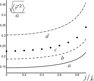
FIG. 1.: The mean-square fluctuations of a FL with zero disorder ($\tilde{\Delta}=0$) for (a) $T=30^{\circ}K$, (b) $T=50^{\circ}K$; and finite disorder ($\tilde{\Delta}/2\pi=0.2$) for (c) $T=30^{\circ}K$, (d) $T=50^{\circ}K$.

The next step is to look for variational solutions which break replica symmetry. The technical details of this calculation are presented in the appendix. Following Goldschmidt[12], we find a solution with 1-step replica symmetry breaking (RSB) for temperatures below a $j_{z}$-independent freezing transition point of

$$T_{cp}\approx(\varepsilon_{0}\xi/\gamma)(\gamma\tilde{\Delta}/2\pi)^{1/3}.$$ (55)

The mean squared fluctuations with the 1-step RSB, again in the limit of $\tilde{B}\ll(\gamma\tilde{T})^{2}$, are obtained from

$$\frac{\overline{\langle\vec{r}\,^{2}\rangle}}{a^{2}}=\gamma\tilde{T}\sqrt{\tilde{B}}\Bigg{\{}\frac{1}{v_{c}\sqrt{1-(j_{z}/j_{c})^{2}}}-\left(\frac{1-v_{c}}{v_{c}}\right)\times$$ (58)

$$\frac{1}{\sqrt{1+{\Sigma}/{\mu}-({j_{z}/j_{c})^{2}}}}+\frac{\gamma\tilde{\Delta}}{4\pi(\gamma\tilde{T})^{3}}\frac{1}{[1-(j_{z}/j_{c})^{2}]^{3/2}}\times$$

$$\left[\frac{1}{v_{c}\sqrt{1-{(j_{z}/j_{c})^{2}}}}-\left(\frac{1-v_{c}}{v_{c}}\right)\frac{1}{\sqrt{1+{\Sigma}/{\mu}-{(j_{z}/j_{c})^{2}}}}\right]^{-2}\Bigg{\}},$$

where the parameters $v_{c}$ and $\Sigma$ are obtained by minimizing the trial free energy expression given in the appendix. This minimization is carried out numerically, and the resulting points for $T=30^{\circ}K<T_{cp}\approx 35.4^{\circ}K$ are plotted in Fig. 1 (c) (and can be compared to those with zero disorder at $T=30^{\circ}K$ in Fig. 1 (a)).

The calculated FL fluctuations are now used to construct an approximate ‘phase boundary’ for the destruction of short-range translational order. According to the Lindemann criterion, ‘melting’ occurs when $\sqrt{\left\langle\vec{r}\,^{2}\right\rangle}\approx c_{L}a$, where $c_{L}$ is a constant of the order of unity. From the replica symmetric solution of Eqn. (54), we obtain a melting field

$$\tilde{B}_{m}=c_{L}^{4}\left[\gamma\tilde{T}_{m}+\left(\frac{\gamma\tilde{\Delta}}{4\pi}\right){\left(\gamma\tilde{T}_{m}\right)^{-2}}\right]^{-2}\left(1-\frac{j_{z}^{2}}{j_{c}^{2}}\right).$$ (59)

In the limit of zero disorder, the above equation reproduces the result $\tilde{B}_{m}=c_{L}^{4}(1-j_{z}^{2}/j_{c}^{2})/(\gamma\tilde{T}_{m})^{2}$ of Ref. [10], and agrees with the expected behavior of $B\sim 1/T^{2}$ for zero current. Using $c_{L}=0.16$, and the same parameters as in Fig. 1, the phase diagram is plotted in Fig. 2. For the portion of the melting line for $T<T_{cp}$, we can no longer use the above analytical form, but must instead rely on the numerical results obtained using Eqn. (58). Interestingly, the melting field shows a maximum around the freezing temperature, even for zero current. Indeed, recent experimental results[14] show a reduction of the melting field for low temperatures.

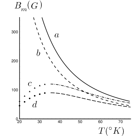
FIG. 2.: ‘Phase diagram’ of FLs for (a) $\tilde{\Delta}/2\pi=0$ and $j_{z}/j_{c}=0$, (b) $\tilde{\Delta}/2\pi=0$ and $j_{z}/j_{c}=0.5$, (c) $\tilde{\Delta}/2\pi=0.1$ and $j_{z}/j_{c}=0$, (d) $\tilde{\Delta}/2\pi=0.1$ and $j_{z}/j_{c}=0.5$.

IV The Transfer matrix method

With or without RSB, the variational method predicts that in the absence of the cage potential ($\mu=0$), the FL is unstable in the presence of infinitesimal $j_{z}$, and cannot be pinned by the impurities alone. We may still question the validity of this conclusion, given the known shortcomings of the variational method. For example, in the absence of current, this method predicts that fluctuations of a FL grow with its length $L$ as $\left\langle\vec{r}\,^{2}\right\rangle\sim L$. In fact, it is known that pinning to impurities results in $\left\langle\vec{r}\,^{2}\right\rangle\sim L^{2\zeta}$, with $\zeta>1/2$[15, 16]. We thus check the results using a numerically exact transfer matrix algorithm applied to a discrete model of the FL.

Consider a FL pinned at one end to the point $(0,0,0)$ on a cubic lattice, and denote the net Boltzmann weight of all paths terminating at the point $(x,y,z)$ by $W(x,y,z)$. We consider only paths that are directed along the $z$-direction, and hence this weight can be calculated recursively as

$$W (z+1,x,y)=\exp\left[{-{V(z,x,y)\over T}-{\mu(x^{2}+y^{2})\over 2T}}\right]\times$$ (60)

$$\Bigg{\{} W(z,x,y)+\Gamma\times$$ (62)

$$\Bigg{[}e^{y{j_{z}}/{j^{\prime}_{c}}}W(z,x+1,y)+e^{-y{j_{z}}/{j^{\prime}_{c}}}W(z,x-1,y)+$$

$$e^{x{j_{z}}{j^{\prime}_{c}}}W(z,x,y-1)+e^{-x{j_{z}}{j^{\prime}_{c}}}W(z,x,y+1)\Bigg{]}\Bigg{\}},$$ (63)

where $j^{\prime}_{c}=2T/\phi_{0}$, and $\Gamma=\exp(-\varepsilon_{1}/2T)$. Note that at each step the path is either straight, or moves by only one step in the transverse direction. Such transverse steps acquire a weight $\Gamma\ll 1$ from the FL elasticity, as well as a direction dependent contribution from the current[17].

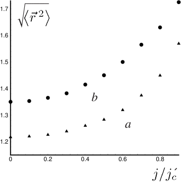
FIG. 3.: The mean-square fluctuations of a FL with $\Gamma=1$, confined to a cage of $\mu/T=0.2$, as a function of the reduced current $j_{z}/j^{\prime}_{c}$, for (a) zero disorder; and (b) binary random potentials chosen from $(0.2,2)$.

Starting with the initial values of $W(0,x,y)=\delta_{0x}\delta_{0y}$, successive applications of this recursion relation provide the weights $W(x,y,z)$ at subsequent layers, which can then be used to calculate the (exact) degree of fluctuations $\left\langle\vec{r}\,^{2}\right\rangle=\left\langle x^{2}+y^{2}\right\rangle$, for a particular realization of the random potential $V(x,y,z)$. The results are then averaged over different realizations of the disorder potential. When the FL is confined to a cage ($\mu\neq 0$), $\left\langle\vec{r}\,^{2}\right\rangle$ quickly saturates to a constant value. Fig. 3 shows the dependence of the saturation point on the external current. For this figure, the random potentials $V/T$ were taken from a binary set $(0.2,2)$, and the results averaged over $500$ realization of randomness. Since the microscopic models are different, it is hard to make a quantitative comparison with the replica calculations. The numerical results are certainly in qualitative agreement with the replica estimates depicted in Fig. 1. It is numerically difficult to probe currents close to the critical value, as the large transverse excursions require simulating large lattices.

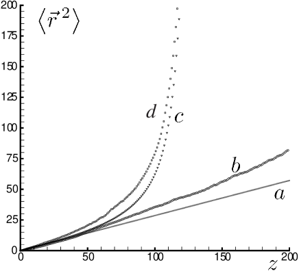
FIG. 4.: Mean-square fluctuations of a FL in a $200\times 50\times 50$ lattice, with (a) $V=0,j_{z}/j_{c}=0$ (b) $V\neq 0,j_{z}/j_{c}=0$ (c) $V=0,j_{z}/j_{c}=0.08$, and (d) $V\neq 0,j_{z}/j_{c}=0.08$.

The most interesting point is the behavior of the FL in the absence of the cage potential. As can be seen from the various limiting curves for $\mu=0$, plotted in Fig. 4, fluctuations no longer saturate, but continue to grow with $z$. When both the current and disorder are zero, the FL behaves as a directed random walk. The straight line in Fig. 4(a) corresponds to $\left\langle\vec{r}\,^{2}\right\rangle\propto t$, as expected in this case. The addition of point disorder changes the scaling of transverse fluctuations[15]. As indicated in Fig. 4(b), the average of $\left\langle\vec{r}\,^{2}\right\rangle$ grows faster than $t$. The results for the binary set $(\{0.2,2\})$ of random potentials $V/T$, averaged over $500$ realization of randomness, are consistent with $\overline{\left\langle\vec{r}\,^{2}\right\rangle}\propto t^{2\zeta}$, with $\zeta\approx 0.6$. This is in agreement with previous results for directed polymers in random media [15]. As indicated in Fig. 4(c) the addition of current to the pure system ($V=0$) leads to instability, and the transverse fluctuations become unbounded. When both binary disorder and current act on the FL, it is again found to be unstable, as depicted in Fig. 4(d). Indeed, we find that even an infinitesimal current can destabilize the FL, and that binary impurities only further increase transverse fluctuations.

Since the use of binary randomness in directed polymer simulations may lead to anomalous results related to percolation[18], we also repeated the simulations using a Gaussian distribution for the disorder potential $V/T$. Such impurities are more effective in pinning the FL, and appear to stabilize it at small scales. However, by varying the width of the lattice or $z$, we see that the FL goes to the edges of the box, indicating its instability. Fig. 5 depicts the dependence of transverse fluctuations on the strength of Gaussian disorder. The fluctuations at short scales are governed by disorder, while at longer scales the current dominates, pushing the FL outward.

FIG. 5.: Transverse fluctuations for $j_{z}/j_{c}=0.1$, with $500$ realizations of the random potential $V/T$ taken from a Gaussian distribution of variance (a) $0$, (b) $2$, and (c) $4$.

V Onset of the Instability

The results of replica and transfer matrix computations can be summarized as follows: A parallel current $j_{z}$ causes instabilities in a flux lattice, or in a single (unconfined) FL. Point impurities appear to only increase the extent of fluctuations, and do not provide stability. On the other hand, if we start with a vortex system pinned by strong point impurities at low temperatures, it is difficult to imagine how an infinitesimal $j_{z}$ can lead to drastic changes in configuration. In this section we discuss the length scales, barriers, and time scales that control the onset of the instability.

Let us first consider a single FL in the absence of point impurities or a confining potential. A normal mode of wavenumber $q_{z}$ has energy proportional to $G_{0}^{-1,L/R}(q_{z})=\varepsilon_{1}q_{z}^{2}\pm\phi_{0}j_{z}q_{z}$, indicating a band of unstable modes for $q_{z}\leq\phi_{0}j_{z}/\varepsilon_{1}$. The instability occurs only on segments of length longer than $\ell^{*}\sim\varepsilon_{1}/(\phi_{0}j_{z})$. (The divergence of $\ell^{*}$ as $j_{z}\to 0$ is cut-off by a finite confining potential.) The simplest equation of motion for the FL relates its local velocity to the force obtained from variations of the Hamiltonian by $d\vec{r}/dt=-\hat{\mu}[\delta{\cal H}/\delta\vec{r}\,]$, where $\hat{\mu}$ is a mobility[10]. The characteristic time scale for the normal modes is now given by $\tau^{-1,L/R}(q_{z})=\hat{\mu}G_{0}^{-1,L/R}(q_{z})$. The time required for the growth of unstable modes diverges as $\tau^{*}\sim\hat{\mu}\varepsilon_{1}^{2}/(\phi_{0}j_{z})^{2}$ for $j_{z}\to 0$. The FL thus appears stable at short times, or at high frequencies $\omega$.

The corresponding analysis for a flux lattice in the absence of impurities is very similar. The (inverse) time scales for growth or decay of normal modes are related to the corresponding propagators $G_{0}^{-1,L/R}$ in Eqn. (13) by a mobility factor. The unstable modes occur over an approximately spherical region centered on $q_{z}\leq\phi_{0}j_{z}/2c$, and the time scale for the onset of instability scales as $\tau^{*}\sim\hat{\mu}c^{2}/(\phi_{0}j_{z})^{2}$.

In the presence of point impurities, we claim that the instability still occurs for length scales larger than $\ell^{*}\sim(\phi_{0}j_{z})^{-1}$. The analytical support for this claim comes from the replica analysis: The best variational propagators (as for example in Eqn. (30)) are proportional to the pure one with the same range of instabilities. There is also numerical support from the transfer matrix calculations: The comparison of Figures 4(c) and 4(d) indicates that the onset of instability is not substantially modified in the presence of the disorder potential. The location of the instability (as determined from such curves for $\left\langle\vec{r}\,^{2}\right\rangle$) is plotted in Fig. 6, and indeed scales as $z^{*}\sim 1/(j_{z}/j^{\prime}_{c})$.

Fig. 6: The behavior of the position for the onset of instability as a function of the current.

In response to the current, the unstable FLs must change configuration at a length scale $\ell^{*}$. This is not easily achieved in the presence of collective pinning by point impurities, and the flux system requires the assistance of thermal fluctuations to overcome the pinning barriers[1, 19]. For a single FL the strength of the collective barriers grows with the length scale as $E_{b}\propto\ell^{\theta}$ with $\theta\approx 0.3$[20]. As $j_{z}\to 0$ the barriers at the length scale for the onset of instability thus diverge as $E_{b}\propto j_{z}^{-\mu}$ with $\mu=\theta$. The probability that the flux system has sufficient thermal energy to overcome such barriers is proportional to the Boltzmann weight $\exp(-{E_{b}/k_{B}T})$. The waiting time for such rare events grows as $\tau^{*}\sim\tau_{0}\exp[(j_{T}/j_{z})^{\mu}]$, where $\tau_{0}$ is a microscopic time scale, and $j_{T}$ is a characteristic current scaling as $T^{-1/\mu}$.

The above arguments essentially follow those of Ref.[19] which considers the response of a collectively pinned flux system to a current perpendicular to the magnetic field. They are equally valid for a collection of flux lines in the vortex glass or Bragg glass phase. The exponent $\theta$ depends on the glass phase considered, its exact value is not as well known as for a single FL. Thus while the equilibrium state of a flux system is destabilized by an infinitesimal $j_{z}$, the time for the onset of such instability diverges. The instability will not be observed if the system is probed at times shorter than $\tau^{*}$, or perturbed by an AC current $j_{z}(\omega)$ with frequency $\omega>\omega^{*}\sim 1/\tau^{*}$. (The latter is in qualitative agreement with the phase diagram presented in Ref.[10].)

A Replica Symmetry Broken solutions for a single FL

In order to find the replica symmetry breaking (RSB) solutions, we parameterize $\sigma_{ab}$ by a function $\sigma(v)$ defined for $0\leq v\leq 1$. The propagators $G_{ab}(q_{z})$ and $G_{aa}(q_{z})$ are also replaced by $G(q_{z},v)$ and $\tilde{G}(q_{z})$, respectively. The stationarity equations are now written as

$$\sigma(v)=\frac{2}{T}\tilde{f}_{p}^{\prime}\left[\frac{1}{2}\left(B^{L}(v)+B^{R}(v)\right)\right],$$ (A1)

where

$$B^{L/R}(v)=2T\int\frac{dq_{z}}{2\pi}\left[\tilde{G}^{L/R}(q_{z})-G^{L/R}(q_{z},v)\right].$$ (A2)

Inversion of the hierarchical matrices gives [13],

$$\tilde{G}^{L/R}(q_{z})-G^{L/R}(q_{z},v)=$$ (A3)

$$\frac{1}{v\left(G_{0}^{-1,L/R}(q_{z})+[\sigma](v)\right)}-\int_{v}^{1}\frac{d\omega}{\omega^{2}}\frac{1}{G_{0}^{-1,L/R}(q_{z})+[\sigma](\omega)},$$ (A4)

where $[\sigma](v)=v\sigma(v)-\int_{0}^{v}d\omega\sigma(\omega)$ as before. Integration over $q_{z}$ now leads to

$$\sigma(v)=\frac{2}{T}\tilde{f}_{p}^{\prime}\left[\frac{1}{v}g\left([\sigma](v)\right)-\int_{v}^{1}\frac{d\omega}{\omega^{2}}g\left([\sigma](\omega)\right)\right],$$ (A5)

where $g\left([\sigma]\right)=T/\sqrt{4\varepsilon_{1}\left(\mu+[\sigma]\right)-\phi_{0}^{2}j_{z}^{2}}$.

For a solution with 1-step RSB, we assume[13, 12],

$$\sigma(v)=\left\{\begin{array}[]{ll}\sigma_{0}&{\rm for}~{}v<v_{c},\\ \sigma_{1}&{\rm for}~{}v\geq v_{c}.\end{array}\right.$$ (A6)

This yields $[\sigma](v)=0$ for $v\leq v_{c}$, and $[\sigma](v)=\Sigma=v_{c}(\sigma_{1}-\sigma_{0})$ for $v\geq v_{c}$. We can substitute the above form in Eqn. (A3) and use the result to evaluate $B^{L/R}$ in Eqn. (A2). Depending on whether $v$ is bigger or smaller than $v_{c}$, we obtain two different values for $B^{L/R}$, which when placed in Eqn. (A1), lead to the self-consistency conditions

$$\sigma_{0} = \frac{2}{T}\tilde{f}_{p}^{\prime}\left[\frac{2T}{v_{c}}\frac{1}{s_{2}}-\frac{2T(1-v_{c})}{v_{c}}\frac{1}{s_{1}}\right]$$ (A7)

$$\sigma_{1} = \frac{2}{T}\tilde{f}_{p}^{\prime}\left[\frac{2T}{s_{1}}\right],$$ (A8)

where $s_{1}=\sqrt{4\varepsilon_{1}(\mu+\Sigma)-\phi_{0}^{2}j_{z}^{2}}$ and $s_{2}=\sqrt{4\varepsilon_{1}\mu-\phi_{0}^{2}j_{z}^{2}}$ (for $j_{z}<\sqrt{4\varepsilon_{1}(\mu+\Sigma)/\phi_{0}^{2}}$). One can evaluate the free energy as a function of the parameters $\Sigma$ and $v_{c}$ of the 1-step RSB solution, as

$$\frac{F}{2L}={\rm const.}+\frac{\tau}{4}\frac{1-v_{c}}{v_{c}}\Bigg{\{}\Sigma\left[1+\frac{\Sigma}{\mu}-\frac{j_{z}^{2}}{j_{c}^{2}}\right]^{-1/2}-$$ (A9)

$$2\mu\left[1+\frac{\Sigma}{\mu}-\frac{j_{z}^{2}}{j_{c}^{2}}\right]^{1/2}\Bigg{\}}-\frac{1-v_{c}}{2T}\tilde{f}_{p}\left(\frac{\tau}{\sqrt{1+{\Sigma}/{\mu}-{j_{z}^{2}}/{j_{c}^{2}}}}\right)$$ (A10)

$$-\frac{v_{c}}{2T}\tilde{f}_{p}\left(\frac{\tau}{v_{c}\sqrt{1-{j_{z}^{2}}/{j_{c}^{2}}}}-\frac{1-v_{c}}{v_{c}}\frac{\tau}{\sqrt{1+{\Sigma}/{\mu}-{j_{z}^{2}}/{j_{c}^{2}}}}\right),$$ (A11)

where $\tau=T/\sqrt{\mu\varepsilon_{1}}$. Variation with respect to $\Sigma$ reproduces the condition $\Sigma=v_{c}(\sigma_{1}-\sigma_{0})$, $\sigma_{0}$ and $\sigma_{1}$ defined in Eqn. (A7). Minimizing the free energy with respect to the $v_{c}$, after some algebraic manipulations, leads to

$$v_{c}=\frac{\tilde{T}}{\tilde{T}_{cp}},$$ (A12)

with $\tilde{T}_{cp}=(\tilde{\Delta}/2\pi\gamma^{2})^{1/3}$. Since $v_{c}\leq 1$, this solution exists only for temperatures lower than a freezing temperature, which is independent of the current and $\mu$. With this value of $v_{c}$ inserted in Eqs. (A7), we can numerically find $\Sigma$ for any temperature and current, and evaluate the FL fluctuations in Eqn. (58).

The natural question is whether there are also solutions with 2-step, or even full RSB. Taking a derivative of Eqn (A5) with respect to $\sigma$, and using the functional form for $\tilde{f}_{p}$, leads after further algebraic manipulations, to a linear relation between $\sigma(v)$ and $[\sigma](v)$. This is inconsistent with the relation $[\sigma](v)=v\sigma(v)-\int_{0}^{v}d\omega\sigma(\omega)$, unless $\sigma$ is a constant (since $\sigma^{\prime}(v)=0$ is always a solution). One the other hand, one can also show by taking two derivatives with respect to $v$, that the only possible solution is $v=v_{c}=\tilde{T}/\tilde{T}_{cp}$, consistent with the 1-step RSB result. We thus conclude that, at least for this particular form for the disorder correlator (and hence $\tilde{f}_{p}$), there is no solution with continuous RSB.

REFERENCES

• [1] G. Blatter et. al., Rev. Mod. Phys. 66, 1125 (1994).
• [2] D. R. Nelson and V. M. Vinokur, Phys. Rev. Lett. 68, 2398 (1992); Phys. Rev. B 48, 13060 (1993).
• [3] L. Balents and M. Kardar, Europhys. Lett. 23, 503 (1993).
• [4] A.I. Larkin and Y.N. Ovchinokov, J. Low Temp. Phys. 34, 409 (1979).
• [5] T. Giamarchi and P. Le Doussal, Phys. Rev. Lett. 72, 1530 (1994); Phys. Rev. B 52, 1242 (1995).
• [6] D. Ertas and D. R. Nelson, Physica C 272, 79 (1996).
• [7] T. Giamarchi and P. Le Doussal, Physica C 363, 282 (1997).
• [8] E. H. Brandt, Rep. Prog. Phys. 58, 1465 (1995); and references therein.
• [9] E. H. Brandt, J. Low. Temp. Phys. 42, 557 (1981); ibid. 44, 33 (1981); ibid. 44, 59 (1981).
• [10] M. Kohandel, M. Kardar, Phys. Rev. B 59, 9637 (1999).
• [11] When the parallel penetration depth $\lambda_{\parallel}$ is finite, our result are applicable only to thin samples with thickness of a few $\lambda_{\parallel}$, or alternatively, only close to the surface of the sample.
• [12] Y. Y. Goldschmidt, Phys. Rev. B 56, 2800 (1997).
• [13] M. Mezard, G. Parisi, J. Phys. I 1, 809 (1991).
• [14] B. Khaykovich, et. al., Phys. Rev. Lett. 76, 2555 (1996).
• [15] M. Kardar, Lectures on Directed Paths in Random Media, Les Houches Summer School (1994).
• [16] Y.-C. Zhang, Phys. Reports 254, 215 (1995).
• [17] The parallel current acts like an imaginary magnetic field[2], and the choice of the weights in Eqn.(60) is similar to those of the gauge field phases used in E. Medina and M. Kardar, Phys. Rev. B 46, 9984 (1992). We explicitly checked that despite the asymmetric appearance of the weights, the FL is equally likely to end in any of the four quadrants.
• [18] H. Chate, Q.-H. Chen, L.-H. Tang, Phys. Rev. Lett. 81, 5471 (1998).
• [19] D. S. Fisher, M. P. A. Fisher, and D. A. Huse, Phys. Rev. B 43, 130 (1991).
• [20] L. V. Mikheev, B. Drossel, and M. Kardar, Phys. Rev. Lett. 75, 1170 (1995); B. Drossel and M. Kardar, Phys. Rev. E 52, 4841 (1995).