[

Very long transients are found in the partially ordered phase of type II of globally coupled logistic maps. The transients always lead the system in this phase to a state with a few synchronous clusters. This transient behaviour is not significantly influenced by the introduction of weak noises. However, such noises generally favor cluster partitions with more stable periodic dynamics.
PACS number(s): 05.45.-a, 05.45.Xt, 05.40.Ca ]

Globally coupled maps (GCM) formed by ensembles of logistic maps have been used as a paradigm of complex collective dynamic behaviour for a decade [1, 2, 3, 4, 5]. Originally, GCM were introduced as a mean-field approach to coupled map lattices [6], but later the nontrivial dynamics and the rich collective phenomenology displayed by that system made it a subject worth of study in itself. One of the main properties of globally coupled logistic maps is the presence of different phases characterized by turbulent (non-synchronized) behaviour, clustering, and global synchronization [2]. The formation of a number of subgroups of synchronized elements out of a symmetrical ensemble has a high relevance for many applications, such as the organization of the immune or the neural system, ecological networks, cell differentiation, and structuring of social hierarchies. Therefore, the GCM phases in which the system displays clustering have been intensively studied [1, 3, 7, 8, 9, 10].

The former studies about the complex collective behavior displayed by GCM are usually based on the classical classification of the phase-space introduced by K. Kaneko [2]. As we report here, the partially ordered phase of type II is equivalent to its neighboring ordered phase, with the only difference that very long transients preceed the achievement of the final attractor. This implies a revision of the phase space of GCM, and shows that there is a strong non-monotonous dependence of the transient length with the system parameters, which has to be taken into account in any numerical study.

The simplest globally coupled discrete-time system is given by

$$x_{i}(t+1)=(1-\epsilon)f{\bf(}x_{i}(t){\bf)}+{\frac{\epsilon}{N}}\sum_{j=1}^{N}f{\bf(}x_{j}(t){\bf)}\;.$$ (1)

where the individual element evolves according to the logistic map $f(x)=1-ax^{2}$, $N$ is the total number of maps and $\epsilon$ specifies the coupling strength. In general, an attractor of this dynamical system is formed by a number ${\cal{K}}$ of synchronous clusters each containing $N_{k}$ elements, $k=1,\dots{\cal{K}}$ and can be characterized by means of the partition $({\cal{K}};\,N_{1}\geq N_{2}\geq\dots\geq N_{{\cal{K}}})$. For convenience, this classification also includes one-element ”clusters” ($N_{k}=1$) that actually correspond to individual non-entrained elements. Thus, the partition ($N;1,1,...,1$) corresponds to the asynchronous state of the entire ensemble, while the partition ($1;N$) represents its fully synchronous state, where all $N$ elements belong to a single cluster. In addition to these two states, the system would generally also have other partitions where a certain number of synchronous groups of elements with $N>{\cal{K}}>1$ are present. The choise of an attractor with a particular partition is determined by the initial conditions. The attractor corresponding to each initial condition is characterized by a certain number ${\cal{K}}_{m}$ of clusters after a transient has elapsed.

The phase space of the GCM (1) has been described by K. Kaneko [2] using the average cluster number ${\overline{{\cal{K}}}}=\sum_{m=1}^{M}{\cal{K}}_{m}/M,$ where the index $m=1,\dots,M$ enumerates the set of employed initial conditions. Four different phases have been identified [2]:

1. Coherent phase. The elements follow the same trajectory ($x_{i}(t)=x_{j}(t)$, $\forall i,\;j;\;t$), forming a single synchronous cluster ($\overline{{\cal{K}}}=1$).

2. Ordered phase. Almost all basin volume is occupied by a few-cluster attractor ($\overline{{\cal{K}}}$ is small and does not grow with $N$).

3. Partially ordered phase. Coexistence of many-cluster and few-cluster attractors ($\overline{{\cal{K}}}$ is large and grows with $N$).

4. Turbulent phase. No synchronization among the elements ($\overline{{\cal{K}}}=N$).

The coexistence of many-cluster and few-cluster attractors has been observed by K. Kaneko in two different parameter intervals. One of them separated the ordered and the turbulent phases. Here the system is in the partially ordered phase of type I, also called the intermittent phase. The other interval lies between the regions occupied by the ordered and coherent phases. In this interval the system is in the partially ordered phase of type II (called the ”glassy” phase in the initial publication [2]). The typical parameter intervals are $1.56<a<1.80$ for $\epsilon=0.3$ (partially ordered phase of type II) [2, 13], and $1.58<a<1.69$ for $\epsilon=0.1$ (intermittent phase) [2, 8, 9, 13].

To compute the asymptotic properties of a dynamical system, one has to ensure that the system has had enough time to approach its final state, i.e. that the dynamical attractor for the given initial conditions has been reached. Slow relaxation is indeed known for some dynamical systems (see, e.g., [11]). The properties of the transients of GCM have not yet been sufficiently investigated. The aim of the present Letter is to systematically study the transient behaviour of GCM, described by equation (1). Our principal result is that inside the whole parameter region, corresponding to partially ordered (”glassy”) phases of type II, only few-cluster attractors are observed after very long transients. This result holds also when weak noises are added. It contradicts to what has previously been reported by K. Kaneko [12].

We performed long runs of up to $T=10^{7}$ iterations and recorded the time at which the final minimum value of ${\cal K}$ was reached in the parameter region corresponding to the partially ordered phase of type II. To this end, the partition $({\cal{K}};\,N_{1}\geq N_{2}\geq\dots\geq N_{{\cal K}})$ was determined every $\Delta t=25-50$ time steps. Double precision real numbers were used in these computations, ensuring the absolute precision of $10^{-16}$. Two elements were taken to belong to the same cluster only if they had exactly the same state within the double computer precision, i.e. if $|x_{i}(t)-x_{j}(t)|<10^{-16}$.

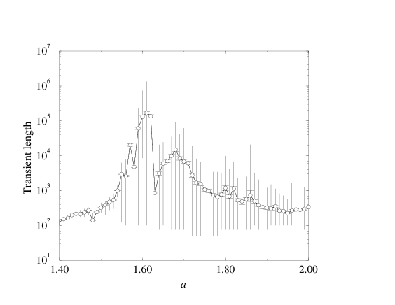
FIG. 1.: Average time required to approach an attractor as function of the control parameter $a$ for the coupling strength $\epsilon=0.3$ in a system of size $N=100$. Averages over 100 different initial conditions are performed. Vertical bars indicate minimum and maximum values of the transient time.

The computed average transient length for $\epsilon=0.3$ as a function of $a$ is shown in Figure 1. We see that the transients may extend up to tens of thousands and even millions of time steps. They become especially long near $a=1.6$. Previous numerical studies [1, 2, 13] were limited to much shorter evolution times (up to $10^{4}$ iterations) and therefore some of the behaviour observed in these studies essentially corresponded to transients. This becomes clear if we compare our Fig. 1 with Fig. 9 in Ref. [2]: A strong increase in the mean number of clusters $\overline{{\cal{K}}}$ was reported exactly where the transient length greatly increases (exceeding $3000$ time steps). Our investigation reveals that, after long transients, only attractors with ${\cal{K}}\leq 2$ are typically found for $a<1.65$, and only attractors with ${\cal{K}}\leq 6$ are observed for $1.65<a\leq 2$. Similar results are also obtained in our calculations for $\epsilon=0.25,\;0.35,$ and $0.4$.

FIG. 2.: Time dependence of the number of clusters in a system of size $N=100$ for the coupling intensity $\epsilon=0.3$ at $a=1.6$ (main plot) and $a=1.8$ (inset), and 30 different initial conditions in each case.

The time dependence of the number of clusters ${\cal K}(t)$ at $\epsilon=0.3$ for 30 different initial conditions is shown in Figure 2 for $a=1.6$ (main plot) and $a=1.8$ (inset). For $a=1.6$, the number of clusters is indeed large during the initial evolution, and comparable with the total size of the system ($N=100$). Later on the number of clusters is slowly decreasing and eventually only attractors with ${\cal{K}}=2$ (but different partitions $N_{1},\;N_{2}$) are found at this value of the parameter $a$. The system evolution at $a=1.8$ is essentially similar, though it is characterized by a much faster convergence to the final states (note the difference by almost two orders of magnitude in the time scales in these two plots). Another difference is that for $a=1.8$ the final states with various cluster numbers ${\cal{K}}=2,\;3$ and $4$ are observed. By averaging over a large number of initial conditions, the time dependence for the relaxation of the mean cluster number ${\overline{{\cal K}}}(t)$ to its asymptotic value ${\cal{K}}$ has been obtained. Figure 3 shows in the logarithmic scale the time dependence of the quantity $\delta{\cal{K}}=$ ${\overline{{\cal{K}}}}(t)-{\cal K}$ for $\epsilon=0.3$ and $a=1.6$. We clearly see that the relaxation is exponential, $\delta{\cal{K}}\propto\exp\{-\beta t\}$.

We have further analysed how the mean transient time $\tau=\beta^{-1}$ depended on the system size $N$. The explored interval of system sizes was $2^{4}\leq N\leq 2^{12}$; we have used several values of $a$ and fixed the coupling strength at $\epsilon=0.3$. We did not find any strong variation of $\tau$ with $N$, i.e. the order of magnitude of $\tau$ did not depend on the system size. The transient length depicted in Fig. 1 is characteristic for almost three decades of variation in the system size $N$.

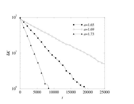
FIG. 3.: Exponential relaxation to the asymptotic state for the coupling intensity $\epsilon=0.3$ and three different values of the control parameter $a$. The slope of the curves (from top to bottom) is $\beta=1.1\times 10^{-4}$, $2.4\times 10^{-4}$, and $5.4\times 10^{-4}$, and errors are of order $10^{-7}$. The system size is $N=100$. Averaging over $M=10^{3}$ initial conditions is performed.

The presence of very long transients indicates that the system may be sensitive to the application of noise. Indeed, for the so-called Milnor attractors even a tiny perturbation would suffice to destabilize the asymptotic state [14]. The existence of Milnor attractors has been discussed both for the partially ordered phase of type II [13] and for the intermittent phase [10]. To analyze the effect of weak random perturbations, we have modified equations (1) by adding a noise term $\eta\;r_{i}(t)$. We have chosen a small noise intensity $\eta=10^{-10}$; independent random numbers $r_{i}(t)\in(-1,1)$ are drawn anew from a uniform distribution for each element and at each time step. Noise prevents the spurious synchronization of elements in the system: If the states of two maps $i$ and $j$ are equal (with computer precision) at time $t$, they will follow identical trajectories for all $t^{\prime}>t$ in a pure deterministic system. When noise is added, spurious attractors are not attained and only robust attractors should be detected.

In the presence of noise the states of elements in a cluster cannot be identical. To define a cluster, we have to choose a certain finite precision $\delta$ and say that elements $i$ and $j$ belong to the same cluster at time $t$ if $|x_{i}(t)-x_{j}(t)|<\delta$ (cf. the respective definition for the case of randomly coupled maps [4]). We have found that the application of weak noise does not qualitatively influence the above-described evolution. Figure 4 shows in logarithmic scale the mean number ${\overline{{\cal{K}}}}(t)$ of clusters as function of time when weak noise is present (all other parameters are the same as in Fig. 3). The system still evolves towards final distributions characterized by a few large clusters. Typically, a slower convergence to the limit value ${\cal{K}}$$=2$ was observed when the noise was acting. Only in a very narrow domain $1.60\leq a\leq 1.62$ did noise seem to prevent convergence to a few-cluster attractor. Note that this area coincides with the maximum transient length in the deterministic case, and is near the boundary where the single synchronous cluster becomes unstable (it is known that the unstabilization of the coherent phase proceeds through a power-law divergence of the transient lenght [4]).

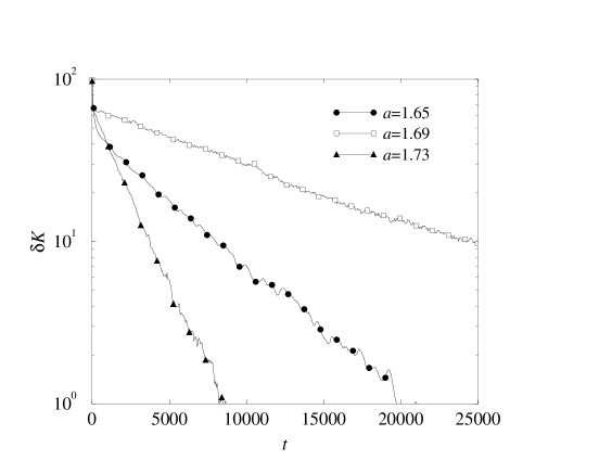
FIG. 4.: Exponential relaxation in GCM added with noise of amplitude $\eta=10^{-10}$ (other parameters as in Fig. 3). The precision is $\delta=\eta^{1/2}$. The slope of the curves (from top to bottom) is $\beta=8\times 10^{-5},\;2\times 10^{-4}$, and $5\times 10^{-4}$.

The dynamics corresponding to a particular cluster partition in our simulations was either periodic or (intrinsically) chaotic. To detect intrinsically chaotic dynamics, local Lyapunov exponents were examined. After a fixed transient of length $T=10^{7}$ we numerically calculated the local Lyapunov exponent

$$\lambda_{m}(\epsilon,a)={\frac{1}{N\tilde{t}}}\sum_{t=T}^{T+{\tilde{t}}}\sum_{j=1}^{N}\log|f^{\prime}(x_{j}(t))|$$ (2)

corresponding to the trajectories $x_{j}(t)$ of elements $j$ for the given initial condition $m$ and parameters $\epsilon$ and $a$. The averaging time was always ${\tilde{t}}=10^{4}$. Positive exponents correspond to chaotic dynamics. The same procedure was used both in the presence and in absence of the noise.

When noise is acting, it may, in principle, induce transitions from one cluster partition to another. Our numerical investigations show, however, that such transitions actually take place in the presence of very weak noises only if the dynamics corresponding to a particular cluster partition is intrinsically chaotic. This observation leads us to a conjecture that Milnor attractors in GCM are, perhaps, only generated by cluster partitions with intrinsically chaotic dynamics. Cluster partitions with periodic attractors are stable against a finite amount of perturbation, while the system leaves with certainty a partition with a chaotic attractor in a finite time when noise is present (see also [10]).

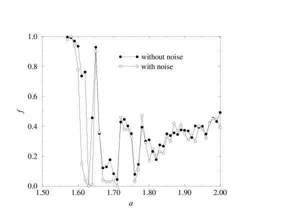
FIG. 5.: Fraction $f$ of initial conditions leading to a chaotic attractor for GCM with and without noise. The parameters are $\epsilon=0.3$ and $N=100$ and we have averaged over $M=10^{3}$ initial conditions.

Interestingly, the addition of noise favors the attainement of periodic attractors. Figure 5 shows the fraction $f$ of initial conditions leading to a cluster partition with (intrinsically) chaotic dynamics with and without noise for the coupling intensity $\epsilon=0.3$, as identified by means of (2). We see that this fraction is strongly reduced in the presence of noise around the parameter value $a=1.61$. To explain this, suppose that the system has approached a cluster partition with chaotic dynamics. Given that any such partition is destabilized even by weak noise, we expect that elements would spend only some time near this attractor, but then one of them would change its cluster affiliation and a new cluster partition would thus be produced. As long as this new partition is also chaotic, the system again easily escapes and the same procedure repeats until a much more stable partition with periodic dynamics is found. This simple argument predicts that, under the action of noise, the system would wander between chaotic Milnor attractors until it eventually finds a robust periodic attractor. If this is indeed so, chaotic attractors would always represent mere transients for sufficiently weak noises. Nonetheless, to test such hypothesis much longer iterations are apparently needed.

Thus, our numerical analysis of globally coupled logistic maps has shown that the collective dynamics of this system in the partially ordered phase of type II is characterized by the presence of very long transients. The asymptotic states of the system in this parameter region are, however, the same as in the ordered phase and include only a small number of synchronous clusters. This conclusion holds even when a small noise, eliminating spurious attractors, is introduced. We have also performed the analysis of dynamical transients in the intermittent phase, i.e. at the interface between the ordered and the turbulent phases, and have found (to be separately published) that in this region the coexistence of few- and many-cluster attractors is indeed observed. These results are important for the general classification of dynamical behaviour in GCM.

The authors acknowledge the financial support from the Alexander-von-Humboldt Foundation (Germany).

REFERENCES

- [1] Kaneko, K., Phys. Rev. Lett. 63, 219 (1989).
- [2] Kaneko, K., Physica D 41, 137 (1990).
- [3] Kaneko, K., Physica D 75, 55 (1994); Physica D 55, 368 (1992).
- [4] Manrubia, S.C. & Mikhailov, A.S., Phys. Rev. E 60, 1579 (1999).
- [5] Żochowski, M. & Liebovitch L.S., Phys. Rev. E 59, 2830 (1999); Zanette, D.H., Europhys. Lett. 45, 424 (1999); Sinha, S., Pérez G., & Cerdeira, H.A., Phys. Rev. E 57, 5217 (1998); Maistrenko, Yu. L., Maistrenko, V. L., Popovych, O., & Mosekilde, E., Phys. Rev. E 60, 1 (1999); Cencini, M., Falcioni, M., Vergni, D., & Vulpiani, A., Physica D 130, 58 (1999); Parravano, A. & Cosenza, M.G., Phys. Rev. E 58, 1665 (1998).
- [6] Kaneko, K., Prog. Theor. Phys. 72, 480 (1984).
- [7] Xie, F. & Hu, G., Phys. Rev. E 56, 1567 (1997).
- [8] Crisanti, A., Falcioni, M., & Vulpiani, A. Phys. Rev. Lett. 76, 612 (1996).
- [9] Kaneko, K., J. Phys. A 24, 2107 (1991).
- [10] Kaneko, K., Phys. Rev. Lett. 78, 2736 (1997).; Physica D 124, 322 (1998).
- [11] Daido, H., Phys. Rev. Lett. 68, 1073 (1992).
- [12] The possibility of very long transients in this region has been mentioned by K. Kaneko in one of his publications [9], but not further explored.
- [13] Kaneko, K., Physica D 77, 456 (1994).
- [14] Milnor, J., Comm. Math. Phys. 99, 177 (1985); 102, 517 (1985).