[

Generalized Phase Field Model for Computer Simulation of Grain Growth in Anisotropic Systems

Abstract

We study the dynamics and morphology of grain growth with anisotropic energy and mobility of grain boundaries using a generalized phase field model. In contrast to previous studies, both inclination and misorientation of the boundaries are considered. The model is first validated against exact analytical solutions for the classical problem of an island grain embedded in an infinite matrix. It is found that grain boundary energy anisotropy has a much stronger effect on grain shape than that of mobility anisotropy. In a polycrystalline system with mobility anisotropy, we find that the system evolves in a non-self-similar manner and grain shape anisotropy develops. However, the average area of the grains grows linearly with time, as in an isotropic system.

]

The effect of anisotropy in energy and mobility of grain boundaries on the kinetics of grain growth and morphological evolution is a relatively unexplored problem. Studies have shown that energy and mobility of a grain boundary depend on the misorientation between the two crystals and the inclination of the grain boundary [2]. In addition, phenomena as segregation of impurities [3] or presence of a liquid phase [4] at the grain boundaries may also result in anisotropy of both energy and mobility.

Although most computer simulations of grain growth have been performed for isotropic cases [5, 6, 7, 8, 9], anisotropy in grain boundary properties has been introduced in a number of simulations, mainly by the Monte Carlo method [10, 11, 12, 13, 14, 15, 16]. For example in the study of texture development during grain growth [10, 11, 12], grains are divided into two types and the contacts between them form three kinds of grain boundaries of either small or large misorientations. To take into account the full range of grain orientations, more general approaches have been proposed [13, 14, 15, 16]. However, all these models consider either misorientation or inclination dependence of grain boundary properties. A simple dislocation model of the grain boundary shows that both energy and mobility of the boundary could depend strongly on both misorientation and inclination [17]. Furthermore, in the models that deal with inclination dependence [15, 16] only a few inclinations are considered and the use of only first neighbors for the calculation of boundary inclination results in an intrinsic energy and mobility anisotropy associated with the discrete lattice used in the simulations [18].

In this paper, to study the kinetics and morphology of grain growth in anisotropic systems, we extend the phase field approach to take into account both inclination and misorientation dependence of grain boundary energy and mobility. The phase field method has been successfully applied for computer simulation of isotropic grain growth[8, 9], phase transformations [19], and solidification [20]. In this model, the polycrystalline microstructure is described by a set of non-conserved order parameter fields $(\eta_{1},\eta_{2},\ldots,\eta_{p})$, each representing grains of a given crystallographic orientation. Microstructural evolution of a polycrystalline system is characterized by the spatio-temporal evolution of the order parameters, via the Ginzburg-Landau-type kinetic equations:

$$\frac{\partial\eta_{i}}{\partial t}=-L\frac{\delta F}{\delta\eta_{i}}\hskip 5.69046pt,\hskip 17.07182pti=1,2,\ldots,p$$ (1)

where $L$ is the kinetic coefficient characterizing the grain boundary mobility, and $F$ is the free energy functional of the form:

$$F=F_{0}+\int d^{3}r[f(\eta_{1}(\textbf{r}),\eta_{2}(\textbf{r}),\ldots,\eta_{p}(\textbf{r}))$$ (2)

$$+\frac{k}{2}\sum_{i=1}^{p}(\nabla\eta_{i})^{2}]$$ (3)

where $f(\eta_{i})$ is the local free energy density and $k$ is the gradient coefficient, which together determine the width and energy of the grain boundary regions.

Several attempts have been made to introduce anisotropic boundary properties into the phase field formulation. For example, in the phase field models of antiphase domain growth and solidification, anisotropy has been introduced by using multiple order parameters based on the underlying crystal symmetry [21, 22]. However, application of these models to grain growth is very difficult due to the fact that the description of the grain boundary is much more complicated, and a quantitative description of a general grain boundary is still lacking. Recently, Kobayashi et al. [23] and independently Luck [24] suggested a different way to extend the phase field model to include anisotropy in grain boundary properties. In their approach, anisotropy is incorporated by introducing an additional variable that describes spatial orientation of the grains. So far, the model has been applied to only quasi-one-dimensional systems with misorientation dependence of grain boundary energy.

In contrast, a simple phenomenological approach has been successfully used to describe the surface energy and mobility anisotropy of crystal surfaces in phase field modeling of crystal growth, where the gradient coefficient $k$ and the kinetic coefficient $L$ have been formulated as functions of crystal surface orientations [20, 25]. In the current paper a similar approach is used to describe grain boundary energy and mobility anisotropy. For the sake of simplicity, we consider tilt grain boundaries between two-dimensional crystals with square lattices, which (ignoring rigid-body translations) can be described by two parameters: relative orientation $\theta$ of the grains (misorientation) and spatial orientation $\phi$ of the boundary with respect to the reference coordinate system (inclination). For crystals with four-fold symmetry and based on simple dislocation models [17], the energy of a low-angle tilt boundary ($\theta\leq 20^{0}$) can be approximated as:

$$E(\theta,\phi)=E_{0}(\left|cos(\phi)\right|+\left|sin(\phi)\right|)\theta(1-ln(\theta/\theta_{m}))$$ (4)

where $\phi=0$ corresponds to the symmetric tilt boundary (see Fig.1), $\theta_{m}$ is the misorientation at which energy is maximum and $E_{0}$ is a constant. The grain boundary energy can be related to the gradient coefficient by $k\propto E^{2}(\theta,\phi)$ [26]. However, as noted by McFadden et al., the gradient coefficient must be a differentiable function with respect to inclination for the Ginzburg-Landau equations to be properly defined [25]. Thus in our simulations the grain boundary energy has been taken in the form:

$$E(\theta,\phi)=E_{0}(1-\delta_{E}cos(4\phi))\theta(1-ln(\theta/\theta_{m}))$$ (5)

which maintains four-fold symmetry in $\phi$, where $\delta_{E}$ is a phenomenological parameter serving as a measure of the degree of anisotropy. The inclination dependence of the energy is similar to the one used in the phase field model of solidification [20]. By choosing $\delta_{E}=0.24$ the same anisotropy ratio as in Eq. (4) is obtained, where the anisotropy ratio $r$ is defined as the ratio of the largest to the smallest grain boundary energy at a fixed misorientation $\theta_{0}$: $r=max{E(\phi,\theta_{0})}/min{E(\phi,\theta_{0})}$.

In the phase field approach to grain growth, grain boundary mobility is characterized by the kinetic coefficient $L$. In contrast to the grain boundary energy, values of the grain boundary mobility are harder to estimate. Qualitatively, in pure materials the higher the defect concentration at a grain boundary the higher its energy as well as its mobility. To investigate qualitatively the effect of mobility anisotropy on the behavior of grain growth, we assume mobility to have the same dependence on misorientation and inclination as the grain boundary energy (Eq.(5)), with a different phenomenological parameter $\delta_{L}$. By varying $\delta_{E}$ and $\delta_{L}$ we can control the anisotropy ratio and investigate the interplay between energy and mobility anisotropy.

The free energy density in Eq.(3) has been taken in the form [8, 9]:

$$f=\sum_{i=1}^{p}[-\frac{a_{1}}{2}\eta_{i}^{2}+\frac{a_{2}}{4}\eta_{i}^{4}]+\frac{a_{3}}{2}\sum_{i=1}^{p}\sum_{j>i}\eta_{i}^{2}\eta_{j}^{2}\hskip 5.69046pt.$$ (6)

In our simulations grain boundary misorientation was considered to be in the range of $0<\theta\leq\Theta$, where $\Theta<\theta_{m}$ Then, misorientation $\theta_{ij}$ between grain $i$ and grain $j$ ($i,j$ = $1\ldots p$, where $p$ is the total number of order parameters used in the simulation) is calculated as $|i-j|\cdot\Theta/(p-1)$. The following values for the phenomenological parameters in Eq.(6) have been used in the simulations: $a_{1}=1.0$, $a_{2}=1.0$, $a_{3}=2.0$. Eq.(1) was discretized using the second order Euler technique on a unit square lattice with $dt=0.1$.

Below we present several applications of our model to systems containing an island grain in an infinite matrix as well as to a polycrystalline aggregate.

Island grain with energy anisotropy. To validate the model against exact analytical results, we first examine shrinkage of an island grain embedded in an infinite matrix. If the grain shrinks in a “self-similar” manner, i.e. maintains its shape while shrinking, Taylor and Cahn [27] have shown that the Ginzburg-Landau equations could be rewritten in the same form as in the isotropic case. As a result, shrinkage kinetics of a grain with arbitrary but self-similar shape should be the same as in the isotropic case. Moreover, they have argued that depending on the form of the gradient coefficient certain complications could occur in the solution of the Ginzburg-Landau equations due to non-convexity in the Wulff plots. Since we are mainly interested in the qualitative behavior of the system and to avoid those complications, we have chosen a grain boundary energy in the form (5) with $\delta_{E}=0.05$ and $E_{0}=1/(1+\delta_{E})$, which gives anisotropy ratio $r_{E}=1.1$. The result of our simulations is presented in Fig.2a. As expected, an initially circular grain transforms to its Wulff shape and then shrinks in a self-similar manner. The extracted kinetics indeed shows linear decline of area with time, in agreement with the theoretical predictions of Taylor and Cahn [27].

Island grain with mobility anisotropy. Following the theoretical analysis of Allen and Cahn [26] for the isotropic case, we obtain a similar relationship for the shrinkage rate of a single island grain with anisotropic boundary mobility:

$$A(t)=A(0)-2\pi k\langle L\rangle_{\phi}t$$ (7)

where $A$ is the area of the grain, and $\langle\ldots\rangle_{\phi}$ represents an average over all possible inclinations. This expression is valid for arbitrary particle shapes and the system does not need to be in a self-similar regime. In the simulations mobility has been taken in the form (5) with $L_{0}=1/(1+\delta_{L})$. In contrast to the case of energy anisotropy, a small mobility anisotropy ($\delta_{L}$=$0.05$, which gives an anisotropy ratio $L_{max}/L_{min}=1.1$) has little effect on the shapes of the grain. Indeed, to reach a similar degree of anisotropy in shape(Fig.2b), we have to introduce a significantly higher mobility anisotropy with $\delta_{L}$=$0.7$, which produces a relative mobility difference (($L_{max}-L_{min})/L_{min}$) $\sim 500$% (while only $10$% difference in energy is required). Experimental observations have shown that the mobility difference could be orders of magnitude larger than the energy diffrence for the grain boundaries [2, 10, 11]. Finally, excellent agreement between the simulation results and the exact analytical solution (7) for the grain shrinkage rate has been observed (Fig.3), which indicates that discretization of the equations does not influence the kinetics.

Island grain with both energy and mobility anisotropy. Next, we discuss the effect of the interplay between the energy and mobility anisotropy of the grain boundary on the shape of a single shrinking island grain. It should be noted that since the functions $E(\phi)$ and $L(\phi)$ have been taken to have the same $\phi$ dependence, for a shrinking island grain energy and mobility anisotropy have opposite effects on the shape. Boundaries with normals in $\frac{\pi}{2}n$ directions have the lowest energies as well as lowest mobilities. Therefore, energy minimization would prefer a shape bounded by the low energy boundaries (Fig.2a), while grain shrinkage with anisotropic boundary mobility would produce a shape bounded by the fastest moving boundaries (Fig.2b). As we mentioned earlier, a small anisotropy in the mobility coefficient ($r_{L}=1.1$) does not have much effect on the shape of the grain; thus the grain shape is dominated by energy anisotropy, giving a shape similar to Fig.2a. On the other extreme a very large mobility anisotropy ($r_{L}=40$) results in diamond-like shapes (Fig.2b). In the intermediate range ($r_{E}$=$1.1$, $r_{L}$=$5.7$), a grain shape with quasi eight-fold symmetry has been observed (Fig.2c), although both energy and mobility as a function of inclination have four-fold symmetry.

Polycrystalline aggregate with mobility anisotopy. For a polycrystalline aggregate, Mullins has shown that the average grain area grows linearly with time if the system evolves in a statistically self-similar (scaling) manner (i.e. all configurations have identical statistics when transformed to the same linear scale by uniform magnification) [28]. However, self-similarity may not hold when boundary properties (energy and/or mobility) are anisotropic [29]. Indeed, our simulations performed on a polycrystalline system with grain boundary mobility anisotropy have shown that grain shapes evolve in a non-self-similar manner, e.g., shape anisotropy develops (Fig.4b). The simulations were performed on $512\times 512$ square lattice with $36$ order parameters. The simulations were started from an isotropic polycrystalline microstructure consisting of $\sim 1000$ grains, obtained from nucleation and growth of crystals from a liquid phase in an isotropic system. Grain boundary mobility anisotropy is introduced according to $L=\theta(1-ln(\theta/\theta_{m}))(1-\delta\cos(2\phi))$, with $\theta_{m}=10^{0}$, $\Theta=5^{0}$ and $\delta_{L}=0.9$, which has two-fold symmetry with respect to $\phi$ and $\phi=\pi/2$ is the fastest growth direction. For comparison, the result obtained from the same initial microstructure in an isotropic system is shown in Fig.4a. Comparing these results it is clear that in the anisotropic case grain shape anisotropy develops. Quantitative analysis of Fig.4b has shown that the inclination distribution of grain boundaries (i.e., boundary length as a function of inclination) is no longer uniform, which suggests that the microstructure is no longer self-similar. However, the average grain area still grows linearly with time as shown in Fig.5. It can be shown analytically [30] that even though self-similarity is not satisfied when grain boundary mobility is anisotropic, the average grain area may still grow linearly with time.

In conclusion, we have studied the dynamics and morphology of grain growth with both energy and mobility anisotropy of grain boundaries using a generalized phase field model that incorporates both inclination and misorientation dependence of grain boundary properties. For a single island grain embedded in an infinite matrix we found that a small anisotropy in grain boundary energy can produce strongly anisotropic grain shapes. In contrast, the mobility anisotropy needs to be significantly stronger to produce similar morphologies. For a polycrystalline aggregate with mobility anisotropy, we found that the average area of the grains grows linearly with time, as in the isotropic case, even though grain shape anisotropy develops, which indicates that the microstructural evolution is no longer self-similar.

We gratefully acknowledge the financial support of NSF under grant DMR-9703044 (AK and YW) and NSF Center for Industrial Sensors and Measurements under grant EEC-9523358 (AK and BRP).

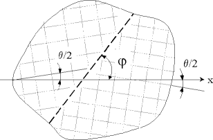
FIG. 1.: Schematic drawing of a tilt grain boundary formed by two crystals with misorientation $\theta$ and inclination $\phi$, measured from the symmetric tilt boundary

$\begin{array}[]{ccc}\epsfbox{fig2a.eps}&\epsfbox{fig2b.eps}\\ (a)&(b)\\ \end{array}$

$\begin{array}[]{c}\epsfbox{fig2c.eps}\\ (c)\\ \end{array}$

FIG. 2.: Shrinkage of a single island grain with (a) energy anisotropy; (b) mobility anisotropy; (c) both energy and mobility anisotropy

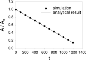
FIG. 3.: Shrinkage kinetics of an island grain embedded in an infinite matrix: comparison between analytical solution Eq.(7) (solid curve) and simulation (solid circles) in the case of anisotropic grain boundary mobility. $A_{0}$ is the initial area of the grain.

$\begin{array}[]{cc}\epsfbox{fig4a.eps}&\epsfbox{fig4b.eps}\\ (a)&(b)\end{array}$

FIG. 4.: Typical microstructures obtained from computer simulations with isotropic grain boundary energy and (a) isotropic and (b) anisotropic boundary mobility with two-fold symmetry with respect to $\phi$

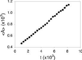
FIG. 5.: Time dependence of the average grain area in a polycrystalline system with grain boundary mobility anisotropy.

REFERENCES

- [1]
- [2] Grain-Boundary Structure and Kinetics, proceedings of the ASM Materials Science Seminar, Milwaukee, Wisconsin, (American Society of Metals, Metals Park, 1980)
- [3] S.J. Bennison and M.P. Harmer, J. Am. Ceram. Soc., 66, C-90 (1983)
- [4] W.A. Kaysser, M. Sprissler, C.A. Handwerker and J.E. Blendell, J. Am. Ceram. Soc., 70, 339 (1987)
- [5] P.S. Sahni, G.S. Grest, M.P. Anderson and D.J. Srolovitz, Phys. Rev. B, 28, 2705 (1983); Acta Metall., 32, 783 (1984); 793 (1984)
- [6] A.C.F. Cocks and S.P.A. Gill, Acta Metall., 44, 4765 (1996)
- [7] H.V. Atkinson, Acta Metall., 36, 469 (1988)
- [8] L.-Q. Chen and W. Yang, Phys. Rev. B, 50, 15752 (1994)
- [9] D. Fan and L.-Q. Chen, Acta Metall., 45, 611 (1997); 1115 (1997)
- [10] V.Yu. Novikov, Acta Metall. 47, 1935 (1999)
- [11] F.J. Humphreys, Acta Metall. 45, 4321 (1997)
- [12] K. Mehnert and P. Klimanek, Scripta Mater. 35, 699 (1996)
- [13] G.S. Grest, D.J. Srolovitz and M.P. Andreson, Acta Metall. 33, 509 (1985)
- [14] N. Ono, K. Kimura and T. Watanabe, Acta Metall. 47, 1007 (1999)
- [15] W. Yang, L.-Q. Chen and G. Messing, Mater. Sci. Eng. A195, 179 (1995)
- [16] Z.-X. Cai and D.O. Welch, Philos. Mag., B70, 141 (1994)
- [17] W.T. Read, Jr., Dislocations in Crystals (McGraw-Hill, New-York, 1953) p. 173
- [18] E.A. Holm, A.D. Rollet and D.J. Srolovitz, in Computer Simulation in Materials Science. Nano/ Meso/ Macroscopic Space and Time Scales, NATO ASI Series E, Applied Sceincies, vol. 308 edited by H.O.Kirchner, L.P. Kubin and V. Pontikis (Kluwer Academic Publishers, Boston, 1996), p. 373
- [19] for a recent review see Y. Wang and L.-Q. Chen, in Methods in Materials Research (John Wiley, New York, 1999); JOM, 48, 13 (1996)
- [20] for a recent review see A. Karma and W.-J. Rappel, Phys. Rev. E, 57, 4323 (1998)
- [21] R.J. Braun, J.W. Cahn, G.B. McFadden and A.A. Wheeler, Philos. Trans. R. Soc. London, 355, 1787 (1997); Acta Metall. 46, 1 (1998)
- [22] A.G. Khachaturyan, Phil. Mag., A74, 3 (1996)
- [23] R. Kobayashi, J.A. Warren and W.C. Carter, submitted to Phys. Rev. Lett.
- [24] M.T. Luck, Proc. R. Soc. London, Ser. A: 455, 677 (1999)
- [25] G.B. McFadden, A.A. Wheeler, R.J. Braun and S.R. Coriell, Phys. Rev. E, 48, 2016 (1993)
- [26] J.W. Cahn and J.E. Hilliard, J. Chem. Phys., 28, 2585 (1958)
- [27] J.E. Taylor and J.W. Cahn, Physica D, 112, 381 (1998)
- [28] W.W. Mullins, J. Appl. Phys., 59, 1341 (1986)
- [29] W.W. Mullins, Acta Metall., 17, 6219 (1998)
- [30] A. Kazaryan, Y. Wang and Bruce R. Patton (to be published)