Determining liquid structure from the tail of the direct correlation function

Abstract

In important early work, Stell showed that one can determine the pair correlation function $h(r)$ of the hard sphere fluid for all distances $r$ by specifying only the “tail” of the direct correlation function $c(r)$ at separations greater than the hard core diameter. We extend this idea in a very natural way to potentials with a soft repulsive core of finite extent and a weaker and longer ranged tail. We introduce a new continuous function $T(r)$ which reduces exactly to the tail of $c(r)$ outside the (soft) core region and show that both $h(r)$ and $c(r)$ depend only on the “out projection” of $T(r)$: i.e., the product of the Boltzmann factor of the repulsive core potential times $T(r)$. Standard integral equation closures can thus be reinterpreted and assessed in terms of their predictions for the tail of $c(r)$ and simple approximations for its form suggest new closures. A new and very efficient variational method is proposed for solving the Ornstein-Zernike equation given an approximation for the tail of $c$. Initial applications of these ideas to the Lennard-Jones and the hard core Yukawa fluid are discussed.

I Introduction

One of the many areas of current research where George Stell has made fundamental contributions is the derivation of integral equations to determine the pair correlation function of a uniform fluid. A number of different integral equations have been proposed [1], often based on the graphical and functional methods pioneered by Stell [2]. However, despite much effort and some impressive successes, there has been a mixed record arising from their use in different applications. For example, while the Percus-Yevick (PY) equation [3, 4] for a fluid of hard spheres is quite accurate, it proved much less successful in describing the structure of systems with longer ranged interactions such as the Lennard-Jones (LJ) fluid [5]. In most cases, we do not have a deep understanding of the reasons for a particular equation’s success or failure. Part of the problem is that standard “closures” of the integral equations usually introduce uncontrolled approximations made mostly for mathematical convenience. Thus it is difficult to assess the physical consequences of the errors introduced and the kinds of interactions for which a particular equation is likely to be accurate.

However, as pointed out by Stell in one of his earliest papers [6], there is a very simple and physically suggestive way to interpret one of the most basic and successful of the integral equations, the PY equation for hard spheres. Stell noted that one can completely determine the pair correlation function $h(r)$ of the hard sphere fluid for all distances $r$ by specifying only the tail or out part of the direct correlation function $c(r)$ (i.e., its value at separations $r>d,$ with $d$ the hard core diameter of the hard spheres). Here $h$ and $c$ are related by the usual Ornstein-Zernike (OZ) equation [1]. See Sec. (III) below for precise definitions and further discussion. If, following OZ, one further assumes that the direct correlation function has the range of the potential, then its out part vanishes for hard spheres. Then the core or in part of $c(r)$ for $r<d$ can be determined directly from the OZ equation and the exact condition imposed by the hard core potential that $h(r)=-1$ for $r<d$. Stell showed that the resulting $h(r)$ computed from the OZ equation is identical to the PY solution for hard spheres. However this simple picture directly applies only to the PY equation for hard spheres.

Stell and other workers [7] generalized this idea to apply to potentials with a hard core and a longer ranged tail by making simple assumptions about the functional form of the out part of $c(r)$ and solving the OZ equation subject to the “core condition” $h(r)=-1$ inside the core. The resulting mean spherical approximation (MSA) and generalized MSA (GMSA) equations have proved useful in a variety of applications. Madden and Rice [8] showed how these ideas could be applied to systems with softer repulsive cores with their soft MSA (SMSA) equation, though the relationship between the original hard core condition and the treatment of soft cores, both in the initial work and in later derivations [1], seems (to us at least!) somewhat unclear. Most recent work on integral equation closures has focused attention on another function, the bridge function (see Sec. VIII C below), which is not simply related to the tail of $c,$ and connections to the earlier work and the insights gained therein have often not been exploited.

In this paper we show how George Stell’s original ideas [6] can be extended in a very natural way to describe more realistic systems with finite ranged soft core interactions and/or weaker and longer ranged (usually attractive) interactions. While some of our conclusions have been noted before, the general perspective and the formalism we develop is new. It gives a unified and physically suggestive way of interpreting and assessing many earlier approaches and ideas and suggests new and simpler approximations. The main idea is to introduce a new continuous function $T(r)$ which reduces exactly to the tail of $c(r)$ outside the (soft) core region. We show that both $h(r)$ and $c(r)$ depend only on the “out projection” of $T(r)$: i.e., the product of the Boltzmann factor of the repulsive core potential times $T(r).$ Essentially then, we have only to prescribe $T$ outside the core, i.e., fix the tail of $c$, to determine $h$ and $c$ everywhere. This conclusion is rigorously true for hard cores, as noted in the original work of Stell and others [6, 7].

We thus make direct contact with a wide class of integral equations related to the PY equation for hard spheres and the MSA and find in a new and more straightforward way equations related to the SMSA of Madden and Rice [8]. Our general approach suggests how to improve the behavior of the SMSA equation at low densities and gives new insights into reasons for the success of some of the most accurate integral equations, including the reference hypernetted chain (RHNC) equation suggested by Lado [9] and the method of Zerah and Hansen [10]. Equally important, many of the inherent limitations of all these methods are clarified.

II System

We consider here the simple case of a one component uniform fluid interacting through a spherically-symmetric intermolecular pair potential $w(r)=u_{0}(r)+u_{1}(r)$, where $u_{0}$ is a harshly repulsive core potential with finite range $\bar{\sigma}$ (so $u_{0}(r)=0$ for $r>\bar{\sigma}$) and $u_{1}$ is a longer-ranged and more slowly varying (usually attractive) potential. We will refer to a system with potential $u_{0}$ alone as the reference system and the potential $u_{1}$ as the perturbation potential. Though many of these ideas can be directly applied to fluids with long-ranged (e.g., Coulomb) forces, several new issues arise there that merit a more detailed discussion, and we will restrict our work here to the case where $u_{1}(r)$ goes to zero at large $r$ faster than $r^{-3}$. We also assume in most of the following that $u_{1}$ is continuous, with at least one continuous derivative at $r=\bar{\sigma}.$ Examples of a pair potential divided in this way are the separations proposed by Ree et al. [11] and by Weeks et al. [12] for the LJ potential.

The local density at a distance $r$ away from a particle fixed at the origin in a fluid with average (number) density $\rho$ is given by $\rho g(r)$, where $g(r)$ is the radial distribution function. In the following, we will use the notation $g(r;[w])$ to indicate the functional dependence of $g(r)$ on the pair potential $w$; the subscripts $0$ will denote the reference system and $d$ a hard sphere system with diameter $d$. Note that $g(r)$ becomes very small in the core region $r<\bar{\sigma}$ because of the repulsive core potential $u_{0}$. In the special case where $u_{0}$ is replaced by a hard sphere interaction $u_{d}(r)$, then $g(r;[u_{d}+u_{1}])=0$ for all $r<d.$ Our goal is to determine quantitatively the pair correlation function $h(r)\equiv g(r)-1$ for the uniform fluid. Important thermodynamic and structural information are contained in $h(r)$ and its calculation has been a major focus of research in the theory of liquids [1].

III Direct Correlation Function

To that end most modern approaches introduce several other related functions. Probably the most fundamental of these is the direct correlation function $c(r)$, defined in terms of $h(r)$ by the Ornstein-Zernike (OZ) equation

$$h(r_{1})=c(r_{1})+\rho\int d{\bf r}_{2}c(r_{2})h(|{\bf r}_{1}-{\bf r}_{2}|)\,.$$ (1)

By iterating this equation $h$ can be represented as a sum of chains of “direct” correlations $c$. For typical short ranged potentials, this suggests that $c$ could be both shorter ranged than $h$ and simpler in structure [1]. Indeed, Ornstein and Zernike [13] assumed that $c$ had the range of the intermolecular potential in developing their theory of correlations near the critical point. While scaling theory shows that $c$ must in fact decay as a power law $r^{-\eta}$ at the critical point, Stell and co-workers [14] have shown that very accurate results can be obtained for thermodynamic properties of the lattice gas surprisingly close to the critical point by assuming $c$ is strictly the range of the potential and choosing its form to yield self-consistent thermodynamic predictions. Moreover, for the long ranged Coulomb potential, assuming that $c$ is proportional to the potential physically incorporates the effects of screening and yields a nonlinear version of Debye-Hückel theory [1].

We refer to the idea that $c$ has (to a good approximation) the range of the potential as the range assumption. A very direct but primitive strategy for calculating $h$ is to guess the form of the presumably simpler function $c,$ perhaps guided by the range assumption, and then determine $h$ from the OZ equation. However, Stell’s interpretation of the PY equation for hard spheres [6] suggests a simpler possibility: perhaps we have to prescribe only the tail of $c$ outside the range of the harshly repulsive core potential $u_{0}$ to determine $h.$ We now develop a general formalism incorporating this idea for a system with potential $w(r)=u_{0}(r)+u_{1}(r)$.

IV Core and Tail Projections Using Continuous Functions

To help us focus on the core and tail parts of functions, we note that the Boltzmann ($e_{0}$) and Mayer ($f_{0}$) functions for the harshly repulsive core potential $u_{0}(r)$ act very nearly as projection operators onto tail or out ($r>\bar{\sigma}$) and core or in ($r<\bar{\sigma}$) subspaces respectively, since

$$e_{0}(r)\equiv e^{-\beta u_{0}(r)}\;\begin{array}[]{cc}\approx 0,&r<\bar{\sigma},\\ =1,&r>\bar{\sigma},\end{array}\hskip 14.45377pt-f_{0}(r)\equiv 1-e^{-\beta u_{0}(r)}\;\begin{array}[]{cc}\approx\;1,&r<\bar{\sigma},\\ =0,&r>\bar{\sigma}.\end{array}\;.$$ (2)

These functions exactly satisfy one property of orthogonal projectors for all $r$ :

$$-f_{0}(r)+e_{0}(r)=1,$$ (3)

and in the tail region $r>\bar{\sigma}$ exactly satisfy the second requirement:

$$-f_{0}(r)\cdot e_{0}(r)=0.$$ (4)

Moreover for small $r<$ $\bar{\sigma}$ well inside the core, the repulsive potential $u_{0}$ is very large and $e_{0}$ essentially vanishes. Thus Eq. (4) also holds in this region to a very good approximation.

However, for soft cores there is a transition region for $r$ near $\bar{\sigma}$ where the r.h.s. of Eq. (4) differs significantly from zero. Thus strictly speaking the functions $-f_{0}$ and $e_{0}$ are not true projection operators over all space. Rather they divide space into two parts: a tail or out part, and a core or in part. The latter is comprised of a transition region for $r$ near $\bar{\sigma}$ and an effective hard core region at smaller $r$. The theory for soft cores we develop works best when the spatial extent of the transition region is much smaller than $\bar{\sigma}$, as is the case for harshly repulsive interactions. In the special case where there is a hard core potential $u_{d}$, the width of the transition region vanishes, Eq. (4) holds exactly for all $r,$ and the corresponding functions $-f_{d}$ and $e_{d}$ are true projection operators. Our theory for soft cores will go over smoothly to that for hard cores in the limit of increasing steepness of the soft core potential.

We now rewrite our correlation functions in projected form. Though our primary focus has been on the pair of functions $h$ and $c,$ both have discontinuities at $r=d$ when there is a hard core potential $u_{d}.$ It is convenient to introduce two new functions that remain continuous even in this limit and from which we can determine both $h$ and $c$. One such function we will use is well known and was originally used by Stell [6]:

$$t(r)\equiv h(r)-c(r).$$ (5)

$t$ is sometimes referred to as the “indirect correlation function” [15]; its continuity even when the potential has a hard core region is clear since it equals the convolution integral in the OZ equation (1). From this it follows that the first $D$ derivatives of $t$ in a $D$-dimensional system are also continuous at $r=d$ even for a hard core system. For harshly repulsive core potentials it is easy to relate $c$ for $r<\bar{\sigma}$ to the core part of $t$: to a very good approximation in the effective hard core region we have

$$c(r)\approx f_{0}(r)[1+t(r)],\;\;r<\bar{\sigma}.$$ (6)

This equation is exact for a hard core potential where $f_{d}$ and $h_{d}=-1$ for all $r<d.$

To determine $c$ outside the core, we now introduce a second continuous function, which we refer to as the tail function $T(r)$, whose out projection $e_{0}(r)T(r)$ reduces exactly to the tail of $c$ in the out region. In the core space we require that $e_{0}(r)T(r)$ correct the small errors in Eq. (6) occurring in the transition region for soft cores. Thus we require for all $r$ that $T(r)$ satisfy:

$$c(r)=f_{0}(r)[1+t(r)]+e_{0}(r)T(r).$$ (7)

Moreover, since $g=c+1+t,$ we have, using Eqs. (3) and (7)

$$g(r)=e_{0}(r)[1+t(r)]+e_{0}(r)T(r).$$ (8)

We have thus rewritten $c$ and $g$ (or $h)$ in projected form using the new functions $t$ and $T.$ While special cases of these equations have been suggested before [6], the general utility of such a $T$ function does not seem to have been realized. The most important properties of the tail function $T$ are clear from Eqs.(7) and (8): i) it reduces exactly to the tail of $c$ in the out region; ii) both $h$ and $c$ depend on $T$ only through the combination $e_{0}T$; iii) $T$ is continuous and differentiable.

To see that the latter holds, let us define the cavity distribution function $y(r)$ in the usual way [1] : $y(r)\equiv e^{+\beta w(r)}g(r)$. Simple analysis like that mentioned above for $t(r)$ (see, e.g., Ref. [4]) shows that $y(r)$ is a well-defined continuous function of $r$ with several continuous derivatives even when $w$ itself has a hard core region or other discontinuities. Using Eq. (8) we immediately get that

$$y(r)=[1+t(r)+T(r)]/e_{1}(r).$$ (9)

Here $e_{1}(r)\equiv e^{-\beta u_{1}(r)}$. Since $y(r)$ and $t(r)$ are continuous and differentiable and the perturbation tail function $e_{1}(r)$ can be constructed to be continuous and differentiable even across a hard core region, it follows that $T(r)$ is continuous and differentiable . When the potential has a hard core, Eq. (9) can alternatively be used to define $T(r)$ for all $r$ in terms of the more familiar functions $y,$ $t,$ and $e_{1}.$

V Basic Result

Now we can refine the primitive strategy of guessing $c$ and using the OZ equation to calculate $h,$ by reexpressing everything in terms of $t$ and $T.$ See the Appendix for numerical details. In principle, if we prescribe $T(r)$ for all $r$ then $t(r)$ can be completely determined from the modified OZ equation. However, we see from Eqs. (7) and (8) that since both $g$ and $c$ (and hence also $t$) depend only on $e_{0}T,$ the results are very insensitive to any errors we make in prescribing $T$ in the core space $r<\bar{\sigma}$. This is obvious in the effective hard core region where $e_{0}$ essentially vanishes. In the narrow transition region, since $T$ is continuous and differentiable, its values there can be accurately determined by extrapolation from those for $r\gtrsim\bar{\sigma}.$ In effect then we only have to prescribe the out part of $T,$ i.e., the tail of $c$, to determine both $h$ and $c$ everywhere. This generalizes Stell’s argument [6] for the hard core PY equation. In the Appendix we introduce a new and very efficient variational method that allows us to determine numerically both $h$ and $c$ from the OZ equation given some approximation for the out part of $T(r).$ This will allow us to find accurate solutions to many standard integral equations in a very simple way.

Note from Eq. (9) that the tail of $c$ is not sufficient to determine $y(r).$ Its values for small $r$ in the effective hard core region depend directly on $T(r)$ there and we cannot expect that extrapolation from the out part of $T$ alone will give accurate results for $T(r)$ well inside the core. From this perspective, the calculation of $y(r)$ (and other closely related functions such as the bridge function $B(r)\equiv\ln y(r)-t(r)$ discussed below in Sec. VIII C) is a much more difficult problem, requiring the accurate determination of both the out and core parts of $T(r).$ Fortunately the latter problem does not have to be solved to find accurate results for $h$ and $c.$ This point was emphasized by Stell for the hard sphere system [6], and we see it holds true much more generally.

VI Relation to Previous Work

Stell’s original work [6] was designed to provide information about the PY equation for a system with the general pair potential $w(r).$ To that end, he introduced a set of equations very similar in form to Eqs. (7), (8), and (9), but with the crucial difference that the Boltzmann and Mayer functions $e$ and $f$ for the full potential $w$ appear, where

$$e(r)\equiv e^{-\beta w(r)}=e_{0}(r)e_{1}(r)\;;\hskip 14.45377ptf(r)\equiv e^{-\beta w(r)}-\;1=f_{0}(r)+e_{0}(r)f_{1}(r)\;.$$ (10)

Here $f_{1}(r)\equiv e^{-\beta u_{1}(r)}-\;1$. Note that $f$ has the range of the full potential and $-f$ and $e$ no longer approximate projection operators onto core and tail regions. Stell’s equations can be written as

$$c(r)=f(r)[1+t(r)]+e(r)d(r),$$ (11)

$$g(r)=e(r)[1+t(r)]+e(r)d(r),$$ (12)

$$y(r)=1+t(r)+d(r).$$ (13)

Eq. (13) can be taken as the definition of the function $d(r)$ (we use Stell’s notation; this should not be confused with the hard sphere diameter). Despite the superficial similarity of these equations to our Eqs. (7), (8), and (9), $d(r)$ in general has very different properties than our analogous function $T(r).$ In particular, $d(r)$ does not reduce to the tail of $c$ in the out region and is likely to have a more complicated oscillatory structure. The main utility of Eqs. (11), (12), and (13) is in analyzing the PY equation: Stell was able to show that the usual formulation of the PY equation for a general potential results from the approximation $d(r)=0$. Unfortunately there is little reason to believe this approximation is generally accurate.

However, in the special case of hard core interactions where $w(r)=u_{d}(r)$ , Eqs. (11), (12), and (13) reduce to our Eqs.(7), (8), and (9), and $d_{d}(r)=T_{d}(r).$ The approximation $d_{d}(r)=0$ in the out region for hard spheres then can be motivated by an application of the range assumption for the tail of $c$. This assumption alone is enough to determine the accurate PY solution for $h_{d}(r)$. The range ansatz $d_{d}(r)=0$ for $r>d$ is exact in one dimension ($D=1$) and hence yields the exact $h_{d}(r)$. In $D=3$, the first errors in $h_{d}^{PY}(r)$ show up at $O(\rho^{2})$ in a density expansion. Overall $h_{d}^{PY}(r)$ remains remarkably close to the results of computer simulations even at higher densities, with small errors most noticeable near contact and at the first minimum for densities near the fluid-solid transition [1]. As noted by Stell [6], all that is required to calculate $h_{d}(r)$ in general is an expression for $d_{d}(r)$ in the out region. Essentially exact results for $h_{d}(r)$ can be obtained from the generalized MSA (GMSA) of Waisman and Lebowitz [16], which assumes the existence of a small short-ranged (Yukawa-like) tail in $c_{d}(r)$ for $r>d$. Parameters in the tail are chosen so that $h_{d}$ gives results for the pressure and compressibility that fit simulation data. The basic picture suggested by the range assumption that the tail of $c_{d}$ has a simple structure and is small and much shorter ranged than $h_{d}$ seems to be well established.

Stell [6] also noted that the extrapolation of the PY approximation $d_{d}(r)=0$ deep into the core space is a separate and much less accurate approximation. For example, the resulting PY expression for $y_{d}(r)$ given by Eq. (13) with $d_{d}(r)=0$ for all $r<d$ can have large errors at small $r$ for $D=1$ even though the PY result for $h_{d}(r)$ is exact. (While $d_{d}(r)$ is continuous and differentiable at $r=d$ higher derivatives are discontinuous, leading to a large positive value at small $r$ for the exact $d_{d}(r)$ at high density.) This strongly suggests that the calculation of $h_{d}$ and $y_{d}$ should be logically separated [17]. Of course, $y_{d}$ is an interesting function and additional properties like the chemical potential can be obtained from it [1]. However, a focus on $h_{d}$ and $c_{d}$ alone permits a very simple theory, and one can use results for the pressure and compressibility from $g_{d}(r)$ and $c_{d}(r)$ and thermodynamic relations to calculate other thermodynamic properties. In particular, in this approach the chemical potential should be calculated by integrating the pressure, and not from the very inaccurate value for $y_{d}(0)$ given by extrapolating $d_{d}(r)=0$ deep into the core space. By introducing the tail function $T(r)$ and the system of equations (7), (8), and (9), we have been able to extend these important ideas of Stell for hard sphere systems [6] to systems with more general interactions.

VII General Properties of the Tail Function

We now describe some general properties of $T(r)$. Using Eqs. (7), (8), and (9), this can be rewritten exactly as

$$T(r)=c(r)-f_{0}(r)e_{1}(r)y(r),$$ (14)

explicitly showing that $T$ reduces to the tail of the direct correlation function in the out region, but has a different form in the core region. To focus on the changes induced by the perturbation potential $u_{1}$, it is useful to define the excess quantities:

$$\Delta T(r)\equiv T(r)-T_{0}(r),$$ (15)

where $T_{0}$ is the exact $T$ function for the reference system, with similar definitions for other excess functions such as $\Delta h$ and $\Delta c.$ According to the range ansatz $T_{0}$ is zero in the out region, and we expect that the exact $T_{0}$ will in general be small and vanish rapidly at larger $r$ outside the core. Thus in the out region $T(r)\approx$ $\Delta T(r),$ and is mainly determined by the potential tail $u_{1}(r)$.

Based on an analysis by Stell [18], it is generally believed that away from the critical point the asymptotic form of $c(r)$ at large $r$ is

$$c(r)\sim-\beta u_{1}(r).$$ (16)

For system with a weak and slowly varying potential tail $u_{1}$ that goes smoothly to zero at large $r$ this is consistent with the idea that the OZ equation should reduce to linear response theory far from the core region. Here $\beta\$is the inverse of Boltzmann’s constant times the temperature. Thus we expect $\Delta T(r)\sim-\beta u_{1}(r)$ far from the core.

At very low density $\rho$ graphical expansion methods show that the exact form of $c(r)$ for interaction potentials going to zero faster than $r^{-3}$ can be written as:

$$c(r)=f(r)[1+\rho\Lambda(r)]+O(\rho^{2}),$$ (17)

where

$$\Lambda(r_{12})=\int d{\bf r}_{3}f(r_{13})f(r_{32}).$$ (18)

Note that the range assumption for $c$ is rigorously true at low density. Similarly it is easy to show that

$$t(r)=\rho\Lambda(r)+O(\rho^{2}),$$ (19)

$$y(r)=1+\rho\Lambda(r)+O(\rho^{2}),$$ (20)

and

$$T(r)=f_{1}(r)[1+\rho\Lambda(r)]+O(\rho^{2}).$$ (21)

It follows from Eq. (21) that $T_{0}(r)=0+O(\rho^{2})$.

VIII Closures and the Tail Function

Most integral equation theories for $h(r)$ are based on the idea of a closure [1]: a second relation between $h$ and $c$ which, when combined with the OZ equation, allows one to solve for the values of $h$ and $c$. However most closures are expressed in terms of more complicated functions like $y(r)$ or $B(r)$ and their form is usually determined by mathematical considerations. See, e.g., Sec. (VIII E) below. The above results show that to calculate $h(r)$ we can focus on the simpler projected function $e_{0}(r)T(r),$ determined essentially only by the tail of $c(r).$ An exact choice will yield an exact $h$ and approximate choices can be motivated by the range ansatz and the general supposition that the tail of $c$ has a simple structure. As discussed in the Appendix, we can also exploit the relatively simple nature of the out part of $T(r)$ in the numerical solution of the resulting integral equations. Other standard closures can be reinterpreted and sometimes simplified by looking at their predictions for the tail of $c.$

A Soft Mean Spherical Approximation

Probably the simplest such prediction directly yields the SMSA integral equation [8]. The SMSA assumes that the limiting linear response value for the tail of $c$ given in Eq. (16) holds for all $r$ in the out region. Thus we set

$$e_{0}(r)T^{SMSA}(r)=e_{0}(r)[-\beta u_{1}(r)]$$ (22)

in Eqs. (7) and (8). In the out region we have $T_{0}^{SMSA}=0$ and $\Delta T^{SMSA}=-\beta u_{1}(r)$. The resulting expressions for $h$ and $c$ can easily be shown to be equivalent to the original SMSA results, which were written in a different form. If $u_{1}=0$ then the SMSA reduces to the PY equation for the reference system. The approximation $T_{0}^{SMSA}=0$ in the out region again can be motivated by the range assumption. When $u_{0\text{ }}$is replaced by a hard core potential $u_{d}$ then Eqs. (7) and (8) with Eq. (22) reduce to the original hard core MSA. This derivation and interpretation of the SMSA and its relation to the MSA seems much simpler than that found in previous work.

One way to improve the SMSA is to improve its description of repulsive forces. Equation (22) sets $T_{0}^{SMSA}=0$ in the out region. If a more accurate expression for $T_{0}$ is known this could be used along with the MSA approximation $\Delta T^{SMSA}=-\beta u_{1}$ in the r.h.s. of Eq. (22). For hard cores the GMSA [16] should give a very accurate expression for $T_{d}(r).$ Its use in the r.h.s. of Eq. (22) for a system with potential $w=u_{d}+u_{1}$ would yield a theory essentially equivalent to the optimized random phase (ORPA) theory of Andersen and Chandler [19], where exact hard sphere correlation functions are supposed to be used along with a MSA treatment of $u_{1}$.

The SMSA gives rather accurate results for the high density LJ fluid and correctly describes the qualitative changes in $\Delta h\equiv h-h_{0}$ induced by $u_{1}.$ However, it is much less accurate at low densities. This can be understood since Eq. (22) does not reduce to the exact result, Eq. (21), at low densities. An improved theory would result from approximations for $T(r)$ that interpolate between the exact low density limit, Eq. (21), and Eq. (22) at high density. We will describe several such theories below.

B PY and HNC Equations

Other integral equation closures can be reexpressed in terms of their predictions for the out part of $T$. In many cases this can give us insights into their strengths and weaknesses. For example, by rewriting the standard expression $g^{HNC}=\exp(-\beta w+t)$ given by the hypernetted chain (HNC) equation [1] in the projected form of Eq. (8), we find that the HNC closure predicts

$$T^{HNC}=\exp(-\beta u_{1}+t)-(1+t).$$ (23)

This agrees with the exact Eq. (21) at low density. However, when applied to the reference system, Eq. (23) predicts that $T_{0}^{HNC}=\exp(t_{0})-(1+t_{0}).$ Since $t_{0}$ is large and oscillatory at higher density in the out region, this strongly violates the range assumption. Indeed the HNC equation gives very poor results for a dense hard sphere system. Experience has shown that the HNC closure does a much better job of describing slowly varying interactions, and for systems with long-ranged Coulomb forces it is often the theory of choice [1]. As discussed below one of the most accurate integral equation theories, the RHNC theory [9], combines a HNC treatment of the more slowly varying potential $u_{1}$ along with an (in principle) exact treatment of reference system correlations.

The PY closure for the reference system incorporates the range assumption and gives a much better description of reference system correlations than does the HNC. However, for the full system it predicts for the out part of $T$:

$$T^{PY}=f_{1}(1+t).$$ (24)

This again agrees with Eq. (21) at low density. However at higher density the oscillations in $t$ and the strong nonlinear dependence on the perturbation potential will yield a larger and more oscillatory tail for $c$ than suggested by the SMSA in Eq. (22). In practice the simple linear response form of the SMSA gives much more accurate results at high density [8].

C Bridge Function

Most recent integral equation closures focus attention on another continuous and differentiable function, the bridge function $B(r)$, which can be defined formally as [1]

$$B(r)\equiv\ln y(r)-t(r).$$ (25)

Thus $g(r)\equiv\exp[-\beta w(r)+t(r)+B(r)].$ $B(r)$ represents the sum of a well-defined set of Mayer cluster diagrams, and the HNC equation results from the approximation $B(r)=0$. $B$ plays a role analogous to our function $T$ in generating closures, and we shall see that some of its relevant properties can be understood more easily from those of $T.$ Thus one can represent $h$, $c$, and $y$ in terms of the pair of functions $B$ and $t$. If $B$ is specified by some closure ansatz, then these functions can be calculated using the OZ equation.

Alternatively, using Eqs. (7), (8), and (9), we can exactly express $B$ in terms of $t$ and $T$:

$$B(r)=\ln[1+t(r)+T(r)]-[t(r)-\beta u_{1}(r)].$$ (26)

Thus $B$ depends on $T$ itself rather than the projected function $e_{0}T$, and in that sense is a more complicated function than $h$ or $c.$ Indeed determining its form, particularly inside the core, has proved a very difficult challenge both for theory and simulation, and definitive results are still not known [20]. However, since the out part of $B$ in Eq. (26) can determine the out part of $T$, we can effectively concentrate only on the out part of $B$ if we restrict ourselves to theories for $h$ and $c.$

In general, the out part of $B$ has a rather complicated oscillatory structure. For example, for the reference system we have exactly in the out region, using the definition of $t$, and the equality of the tails of $c$ and $T,$

$$B_{0}(r)=\ln[1+h_{0}(r)]-h_{0}(r)+T_{0}(r),\;\;r>\bar{\sigma}.$$ (27)

Since the exact $T_{0}$ is almost certainly small and very short ranged, as suggested by the range ansatz and the success of the PY equation for repulsive forces, $B_{0}$ will have longer ranged oscillations determined by those of the pair correlation function $h_{0}$. Setting $T_{0}=0$ in Eq. (27) yields the PY expression for the reference system bridge diagrams.

However, in many cases the oscillatory tail of $B(r)$ for the full system seems to depend only weakly on the perturbation potential $u_{1}(r),$ so that $B(r)$ $\approx$ $B_{0}(r).$ This idea has been called the universality of the bridge function [21], with $B_{0}$ often approximated by $B_{d}$, the bridge function of an appropriately chosen hard sphere system . The following argument gives some insight into why this could be a reasonable approximation for the out part of $B.$ Analogous to Eq. (27), we have exactly

$$B(r)=\ln[1+h(r)]-h(r)+[T(r)+\beta u_{1}(r)],\;\;r>\bar{\sigma}.$$ (28)

At high density, the structure is dominated by repulsive forces for systems with short-ranged interactions [12] and it is a fairly good approximation to set $h(r)\approx h_{0}(r)$ (“universality” of the correlation functions!) Moreover the success of the SMSA suggests that $T(r)\approx-\beta u_{1}(r)$ and $T_{0}(r)\approx 0$ are also reasonable approximations in the out region. Then Eqs. (27) and (28) yield $B(r)\approx B_{0}(r)$ in the out region. Note that this result is exact at low density since $B=0+O(\rho^{2}).$ Thus for this class of systems, we can arrive at the idea of approximate bridge function universality outside the core using the more physically transparent arguments of the SMSA. Differences in the results for the two theories should be small at high density. It can be seen using the general expression for $B$ in Eq. (26) that these arguments do not hold for the core part of $B$ and we see no reason to expect any such “universality” at higher densities there.

D RHNC Equation

Alternatively, if we assume it is a good approximation to set $B(r)\approx B_{0}(r)$ in the out region, then for systems where $h(r)\approx h_{0}(r)$ we have $T(r)\approx-\beta u_{1}(r)$ from Eqs. (27) and (28), which is the SMSA closure. At low density $h(r)\approx h_{0}(r)$ is not accurate, and the true $T(r)$ must differ significantly from the SMSA prediction. Indeed using the exact low density forms for $h$ and $h_{0}$ along with $B(r)=B_{0}(r)$ in Eqs. (27) and (28) yields the exact low density form for $T$ given in Eq. (21). Thus a theory incorporating $B(r)\approx B_{0}(r)$ in the out region will give exact results for $h$ at low density and should give results at high density close to those of the accurate SMSA.

This is what is done in the RHNC theory of Lado [9], and overall this is one of the most successful integral equation methods known. The standard RHNC closure can be written as

$$g^{RHNC}(r)=\exp[-\beta w(r)+t(r)+B_{0}(r)],$$ (29)

thus replacing the exact bridge function $B$ by $B_{0}.$ To describe its predictions in terms of $T,$ it is convenient to consider excess functions like that defined in Eq. (15). We find

$$e_{0}(r)\Delta T^{RHNC}(r)=g_{0}(r)\{\exp[-\beta u_{1}(r)+\Delta t(r)]-1\}-e_{0}(r)\Delta t(r).$$ (30)

Note that we only require accurate values for $g_{0}(r)$ and not for $B_{0}(r)$ well inside the core to determine this fundamental quantity in our approach . A numerical solution can be found using the general variational method described in the Appendix.

To examine the relation between the RHNC and the SMSA more quantitatively, let us define

$$\Delta T(r)\equiv-\beta u_{1}(r)+\xi(r).$$ (31)

For the SMSA $\xi^{SMSA}(r)=0$ in the out region. We find that in the out region $\xi^{RHNC}(r)$ can be written exactly as

$$\xi^{RHNC}(r)=\Delta h(r)-\ln[\Delta h(r)/g_{0}(r)+1],\;\;r>\bar{\sigma}.$$ (32)

This agrees with exact results from Eqs. (21) at low density and corrects the poor behavior of the SMSA there. At higher density, $\xi^{RHNC}$ represents an additional oscillatory component in the tail of $T$ when compared to the SMSA.. However, when $\Delta h$ is small, as is generally the case at high density for the systems we consider, then $\xi^{RHNC}$ is small (with $\xi^{RHNC}$ vanishing whenever $\Delta h(r)=0$). Thus $\Delta T^{RHNC}\approx\Delta T^{SMSA}=-\beta u_{1}$ in the out region at high density, as argued above.

E Unique Function Ansatz

Several workers have tried to find more accurate expressions for $B(r)$ by assuming it is some unique local function [22] of $t(r),$ as suggested by several approximate closures that gave good results for systems with short ranged repulsive interactions [23]. LLano-Restrepo and Chapman (LC) showed for systems with an attractive potential tail $u_{1}$ that this assumption was generally inaccurate at small $r$ in the core region and also was inaccurate at high density outside the core [24]. They proposed that there could exist some “renormalized” function $\tilde{t}(r)$ involving $u_{1}$ such that $B$ is a local function of $\tilde{t}.$ They found that the choice

$$\tilde{t}(r)=t(r)-\beta u_{1}(r)$$ (33)

gave accurate results at high density in the out region for the LJ fluid. This is precisely what would have been suggested by applying the SMSA closure $T(r)=-\beta u_{1}(r)$ to the exact Eq. (26) in the out region.

However, the SMSA approximation for $T$ is not accurate well inside the core space and indeed the renormalized function gave poor results there. Moreover the SMSA approximation for $T$ is inaccurate at low density where the exact $T$ reduces to $f_{1}.$ Indeed this shows that the local function ansatz for $B$ cannot in general be correct even outside the core. Duh and Haymet [20] and Duh and Henderson [25] have proposed different density dependent separations of the total potential: $w(r)=\tilde{u}_{0}(r;\rho)+\tilde{u}_{1}(r;\rho)$, with “reference” ($\tilde{u}_{0}$) and “perturbation” ($\tilde{u}_{1}$) parts chosen such that Eq.(33), now defined with $\tilde{u}_{1},$ could give more accurate results for $B$ as a local function of $\tilde{t},$ even well inside the core where LC’s original suggestion most noticeably failed. It is clear from Eq. (26) that the unique function ansatz can give exact results at low density only if the perturbation $\tilde{u}_{1}(r;\rho)$ vanishes as $\rho\rightarrow 0$ since then $T\rightarrow T_{0}=0,$ as shown in Refs. [20] and [25]. Assessing the nature of errors induced by the unique function approximation in general remains a very difficult task. For our purposes here it seems simpler and more direct to retain the original physically motivated separation and focus instead on the out part of $T,$ whose density dependence is such that $T$ reduces to $f_{1}$ at low density while approximating $-\beta u_{1}$ at high density.

IX Closures Satisfying Consistency Conditions

A natural idea is to consider more general density-dependent expressions for $T$ that can vary between these limits, as suggested by the RHNC equation. Parameters in the interpolation function can be chosen to fit simulation data or to satisfy various thermodynamic consistency conditions (Maxwell relations and sum rules) which the exact correlation functions must obey. We first discuss one of the most successful integral equation approaches, the method of Zerah and Hansen (ZH) from this perspective [10], and then introduce a new and simplified method which implements this idea in a very direct fashion. Results seem very promising. Contact is also made with very recent work by Stell and coworkers [26].

A HMSA Equation.

ZH introduced a generalized “HMSA” closure that interpolates nonlinearly between the SMSA closure at small $r$ and the HNC closure at large $r$, with a parameter in the interpolation function chosen to give consistent results for the pressure computed from the virial and compressibility formulas [10]. The choice of the HNC theory at large distances was motivated by its superior behavior for systems with long-ranged forces. The ZH closure can be rewritten as the following expression for $T$ in the out region:

$$T^{ZH}(r)=\frac{\exp\{F_{\alpha}(r)[t(r)-\beta u_{1}(r)]\}-1-F_{\alpha}(r)t(r)}{F_{\alpha}(r)}\;,$$ (34)

where $F_{\alpha}(r)$ is an $r$-dependent interpolation function,

$$F_{\alpha}(r)=1-\exp(-r/r_{\alpha}),$$ (35)

and $r_{\alpha}$ a fitting parameter chosen to achieve thermodynamic consistency. For $F_{\alpha}\rightarrow 0$ ( i.e. for $r/r_{\alpha}\rightarrow 0)$ Eq. (34) reduces to the SMSA closure $-\beta u_{1}$ and for $F_{\alpha}\rightarrow 1$ ( i.e. for $r/r_{\alpha}\rightarrow\infty)$ Eq. (34) reduces to the HNC closure, Eq. (23), though Eq. (35) implies a rather slow transition between these limits for physically relevant values of $r_{\alpha}$.

For the systems we consider here with short-ranged interactions, the important feature of Eq. (34) is not the behavior of the HNC equation at large distances but the fact that at low densities $T^{HNC}$ reduces to the exact result, Eq. (21). ZH found numerically for the LJ fluid that $r_{\alpha}$ decreased as the density tended to zero, so the HNC closure is effectively used at all relevant $r$ at very low density. At higher density $r_{\alpha}$ increases, thus mixing in more and more of the SMSA expression. For example, near the triple point (at a reduced density of 0.85 and a reduced temperature of 0.786) ZH found that $r_{\alpha}=6.25\sigma$[10]. The ZH interpolation scheme provides a mechanism by which one can go between these limits as the density changes while maintaining enough flexibility in the shape of $T$ outside the core that thermodynamic consistency for the pressure can be achieved.

B Tail Interpolation Method

Both the ZH equation and the RHNC equation discussed above in Sec.VIII D give accurate results at both high and low densities by considering some rather complicated density dependent expressions for the out part of $T,$ which in particular involve $t(r).$ See Eqs. (34) and (30). The variational method discussed in the Appendix can be used to solve the OZ equation when the out part of $T$ is a known function of $r$, as is the case for the SMSA approximation. Because of the appearance of the initially unknown function $t(r)$ in the ZH and RHNC expressions for $T(r),$ we cannot use this method alone to solve these equations. However, by making an initial guess for the out part of $T,$ we can iterate until the value of the out part of $T$ does not change. This method combines the standard Picard iteration scheme for the hopefully slowly varying out part of $T$ with the efficient variational method for the core parts of functions. While we have found that this method generally works quite well, it still requires much more computer time than does the direct variational solution of the OZ equation with a known out part of $T.$ Moreover because of the complicated nonlinear nature of the self-consistency condition and the direct interplay between possible oscillations in $t$ and $T$ in the out region it is not clear that self-consistent solutions can always be found for physically relevant states. Indeed the RHNC equation fails in a quite peculiar way [27] close to the vapor-liquid coexistence region.

We now introduce a new method, which we call the tail interpolation method (TIM), that implements the idea of a density dependent interpolation involving $f_{1}$ and $-\beta u_{1}$ very directly, while using a very simple ($t$ independent) expression for the out part of $T.$ We assume the out part of $\Delta T$ can be written as:

$$\Delta T^{TIM}(r)=\alpha f_{1}(r)+(1-\alpha)[-\beta u_{1}(r)],$$ (36)

where $\alpha$ is a (temperature and density dependent) parameter that is chosen so that consistent results for two different routes to one particular thermodynamic quantity are obtained. (To obtain the full $T$ the out part of $T_{0}$ should be added to Eq. (36); often the SMSA-PY approximation $T_{0}=0$ gives sufficient accuracy.) Note that the presumably exact asymptotic form for the tail of $c(r)$ given in Eq. (16) is maintained for any choice of $\alpha$, and $\alpha$ is not required to lie between zero and one. In general, varying $\alpha$ allows us to change the shape of the tail of $c$ at intermediate distances while maintaining the proper asymptotic form, and we use this freedom to achieve partial thermodynamic self-consistency. At low density $\alpha=1$ and, given the relative accuracy of the SMSA, we expect that at high densities smaller values of $\alpha$ will be found.

In this paper we impose consistency between the virial and compressibility routes to the isothermal compressibility. Belloni [28] has shown that this can be implemented very efficiently by differentiating the OZ equation, and our variational method can be easily extended to this case. We have not yet examined in any detail the merits of this choice over other possible consistency conditions. Indeed the SMSA usually gives rather poor results both for the virial pressure and for the compressibility [30], and the energy route is typically used to give more accurate thermodynamic results [26]. It is easy to derive a variational method to impose thermodynamic consistency from the energy route and we suspect this will give even better results. However, in this initial study we have imposed consistency on the isothermal compressibility to see whether self-consistency using the very simple expression for $T(r)$ given in Eq. (36) can improve on the rather poor performance of the SMSA for this quantity. The preliminary data we report in the next section illustrates the basic concept and suggests that further work is indeed merited.

X Numerical Results

We test our approach on two well-studied systems: the hard core Yukawa fluid (HCYF) and the LJ fluid. The HCYF has been the focus of recent theoretical work [26] and represents a system where errors from the treatment of soft cores do not arise, while the LJ fluid is a typical soft core system.

A HCYF

The interaction potential in the HCYF is given by:

$$w^{HCYF}(r)=u_{d}(r)+\epsilon\frac{e^{-z(r-d)}}{r/d},$$ (37)

where $d$ is the hard sphere diameter. We choose $z=1.8/d$, which corresponds to a well-studied system [29, 30]. We have solved the TIM equations using the variational method described below in the Appendix. For greater accuracy in treating the hard sphere correlations at high density, we have included a GMSA like expression for $T_{d}$ in the out region, as described in the Appendix. Only preliminary results are reported here. In Fig. 1 we give values for the compressibility factor $\beta P/\rho$ compared to the results of a MD simulation study [30]. We emphasize that the compressibility factor has been calculated directly from the virial formula for pressure and not obtained through thermodynamic relations from the energy route, as is usually done in ORPA and MSA approaches for greater accuracy. In the inset to Fig. 1 we present the dependence of the TIM self-consistency parameter $\alpha$ on temperature and density. Isotherms $T^{*}=2.0$ and $T^{*}=1.5$ are supercritical, and $T^{*}=1.0$ is subcritical . At low densities $\alpha$ approaches the exact limit $\alpha=1$, while at higher densities $\alpha$ becomes smaller though differing from zero (the MSA limit). The behavior at intermediate densities where $\alpha$ reaches a maximum is interesting and was not anticipated by us. The behavior of the TIM very near the critical point and spinodal lines has not been examined.

To test the accuracy of the correlation functions predicted by the TIM, we compare them to the results of new MC simulations we have carried out . In Fig. 2 we show $h(r)$ given by the TIM, the ORPA, and an even simpler self-consistent approach (SC2) very similar to that used by Stell and coworkers [26], where $T^{SC2}(r)=\alpha[-\beta u_{1}(r)]$, with $\alpha$ is chosen to satisfy self-consistency of the virial and compressibility routes to the compressibility. Since the SC2 tail does not have enough flexibility to reduce to $f_{1}$ at low density, we expect that its correlation functions may be less accurate there. The results show the relatively inaccuracy of the ORPA at intermediate and low densities, with best results seen at high density. The SC2 approach, while giving accurate self-consistent thermodynamics, yields less accurate correlation functions at low densities, as expected.

B LJ fluid

We have also solved the TIM equations for the LJ fluid for a few states, using the WCA separation of the pair potential [12]. For the relatively low density states we study here, the SMSA-PY approximation for the reference system $T_{0}=0$ gives sufficient accuracy. In Fig. 3 we compare predictions of TIM and SMSA approximations to MD simulations results [31]. The states shown correspond to low and moderate densities at about the critical temperature. Again the TIM approach gives notable improvement over the SMSA theory, especially at low densities.

XI Final Remarks

Many issues in the theory of integral equations for fluid structure can be profitably analyzed and interpreted in terms of predictions for the out part of the tail function $T(r),$ i.e., the tail of the direct correlation function. In this paper we have only considered a single component uniform fluid with short ranged interactions. Here the simplest possible MSA linear response approximation relating the tail of $T(r)$ to the perturbation potential $u_{1}(r)$ immediately yields the SMSA theory. For systems with harshly repulsive forces only, the SMSA reduces to the successful PY theory. For systems with a weak potential tail $u_{1}(r),$ the SMSA gives rather accurate results at high density but fails at low density. The behavior at low densities can be greatly improved by introducing a density dependence into the tail of $T(r)$ such that it reduces to the exact low density result of Eq. (21), as is effectively done in the RHNC and HMSA equations. We introduced here a new self-consistent (TIM) method that incorporates this idea in a much simpler form, and the preliminary results for the LJ fluid and the HCYF appear promising.

The success of all these methods at high density arises from the fact that for the systems considered attractive forces have only a relatively small effect on the liquid structure, so that $h(r)\approx h_{0}(r)$ is a fairly good approximation. Put another way, the density fluctuations can be well described by a simple Gaussian theory [37]. When this is not true, as is the case for nonuniform liquids [39], particularly in cases of wetting and drying phenomena, the natural (singlet) generalizations of all these integral equation methods fail[38]. We simply do not know a good enough guess for the tail of $T(r)$ in cases where attractive forces induce such significant structural changes. New approaches based on a self-consistent mean field treatment of the attractive interactions appear more promising here [39].

A more severe test of these ideas and of the utility of integral equations in general for uniform fluids is in applications to systems with long-ranged Coulomb interactions. Here one must deal with fluid mixtures with strong and long-ranged attractive and repulsive interactions, and the correlation functions differ in significant ways from those of any reference system with short-ranged forces. Nevertheless, characteristic properties of systems with long-ranged forces, such as the Stillinger-Lovett moment conditions are very naturally expressed in terms of the tail of the direct correlation function [1]. The RHNC and HMSA approximations have often proved useful here, and even the simple SMSA captures Debye screening, perhaps the most fundamental feature of the long-ranged force problem. We hope that some the ideas presented here for the $T$ function can be extended to long-ranged force systems to provide a more intuitive understanding of the strengths and weaknesses of existing integral equation approaches, and aid in the development of new and simpler approximations.

XII Acknowledgments

It is a pleasure to dedicate this paper to George Stell on the happy occasion of his 65th birthday. This work was supported by NSF Grant No. CHE9528915.

A Variational Method

1 Fixed Tail Function

We can look on the OZ equation (1) as indirectly relating the continuous functions $T(r)$ and $t(r).$ Thus, given $T(r)$ we can in principle solve for $t(r)$ and then determine $h(r)$ and $c(r)$ from Eqs. (7) and (8). We first consider the simplest case, exemplified by the SMSA, where the out part of $T(r)$ is a fixed prescribed function, independent of other correlation functions and/or the density. Then we show how to generalize this approach for an arbitrary choice of $T(r)$, which can be coupled to other correlation functions such as $t(r).$ In the latter application our approach represents a new way to solve standard integral equations, and we believe it offers some notable advantages over conventional methods.

It is easy to rewrite the OZ equation (1) in terms of $t$ and $c.$ Taking Fourier transforms we have

$$\hat{t}(k)=\frac{\rho\hat{c}^{2}(k)}{1-\rho\hat{c}(k)},$$ (A1)

where $\hat{c}(k)$ denotes the Fourier transform of $c(r).$ As noted above, only the “out projection” $e_{0}(r)T(r)$ is actually relevant for $h$ and $c$. Given this, Eq. (7) shows that we need to fix only the “core projection” $f_{0}(r)t(r)$ to determine $c(r)$ for all $r$. In principle, $t(r)$ can then be determined everywhere from the modified OZ equation (A1). A proper self-consistent choice for $t(r)$ inside the core must yield the same functional form when it is computed indirectly using the OZ equation (A1). This requirement can be formulated very efficiently in terms of a variational procedure.

In the following analysis $e_{0}(r)T(r)$ is held constant and variations in all functions are generated solely by variations in $t(r)$ restricted to the core region $r<\bar{\sigma}$. According to Eq. (7), variations of $c(r)$ and $t(r)$ then are linearly related:

$$\delta c(r)=f_{0}(r)\delta t(r).$$ (A2)

To arrive at the proper variational functional, we first formally integrate the r.h.s. of Eq. (A1) with respect to $\hat{c}$, thus arriving at a functional

$$\Phi_{OZ}=-\frac{1}{(2\pi)^{3}}\int\{\rho^{2}\hat{c}^{2}(k)/2+\rho\hat{c}(k)+\ln[1-\rho\hat{c}(k)]\}d{\bf k\;,}$$ (A3)

whose general variation with respect to $\hat{c}$ can be simplified using the modified OZ equation (A1):

$$\delta\Phi_{OZ} = -\frac{1}{(2\pi)^{3}}\int\left[\rho^{2}\hat{c}(k)+\rho-\frac{\rho}{1-\rho\hat{c}(k)}\right]\delta\hat{c}(k)d{\bf k}$$ (A4)

$$= \frac{\rho^{2}}{(2\pi)^{3}}\int\hat{t}(k)\delta\hat{c}(k)d{\bf k\;.}$$ (A5)

Using Parseval’s formula, and considering the special variation of $c$ given by Eq. (A2), we have

$$\delta\Phi_{OZ}=\rho^{2}\int f_{0}(r)t(r)\delta t(r)d{\bf r\;,}$$ (A6)

which expresses the result in terms of the imposed variation of $t$ inside the core. In Eq. (A6), $t(r)$ satisfies the OZ equation (A1). We now consider a second functional of $t$ :

$$\Phi_{dir}=-\frac{\rho^{2}}{2}\int f_{0}(r)t^{2}(r)d{\bf r}$$ (A7)

whose variation directly gives the negative of the r.h.s. of Eq. (A6). Thus by construction, the functional

$$\Phi\equiv\Phi_{OZ}+\Phi_{dir}$$ (A8)

obtained by adding Eqs. (A3) and (A7) is stationary (and reaches its minimum) when the proper self-consistent value for $t(r)$ inside the core is used.

To implement this variational method, we expand the core part of $t(r)$ for $r<\bar{\sigma}$ in terms of Legendre polynomials, orthogonal on $[0,\bar{\sigma}]$:

$$t(r)=\sum_{i=1}^{n}a_{n}P_{n}(r),\;\;r<\bar{\sigma}.$$ (A9)

We choose values of the coefficients $a_{n}$ to minimize the functional $\Phi$ in Eq. (A8). We have used Powell’s quadratically convergent method to implement the minimization procedure [32]. If needed, one could improve this step of the calculation by using conjugate gradient methods. In practice, our implementation is very efficient, and $t$ is smooth enough that it is generally sufficient to use $n\approx 5$ to get highly accurate results. For example, for hard core systems $-(1+t)=c$ inside the core, and the exact solution of PY equation for hard spheres gives a $c$ that is a cubic polynomial [1]. Fast Fourier Transform methods [32] are used in evaluating Eq. (A3).

One important general feature of our method is that we expand the smooth function $t$ inside the core rather than $c.$ As discussed above, for hard core systems these two procedures are equivalent, and our method then reduces exactly to the variational method Andersen and Chandler [19] used to solve the hard core MSA and ORPA equations. However, for soft core systems, while $c(r)$ is simply related to $t(r)$ well inside the core, it changes rapidly in the narrow transition region, close to $r\approx\bar{\sigma}$. Higher order polynomials are required to describe this rapid localized variation of $c$ accurately. This problem becomes more and more severe with increasing steepness of the reference system potential. However $t$ changes smoothly and slowly even in the transition region. This is illustrated in Fig. 4, where we show $t(r)$ and $c(r)$ both for the full LJ system, calculated using the self-consistent TIM method discussed in Sec. (IX B), and for the LJ reference system using the SMSA (PY) approximation. The same qualitative features are seen both at lower and higher densities and using other accurate closures. Previous variational methods proposed for soft core systems [33, 34] have either expanded $c(r)$ inside the core or $h(r)$ itself.

2 Arbitrary Tail Function

To solve integral equations for an arbitrary prescription for $T(r)$ containing initially unknown functions like $t(r)$ (see, e.g., Eqs. (24), (23), and (30) for the PY, HNC and RHNC equations) we can combine the variational technique with an iterative method. First, we make an initial guess $T^{(0)}(r)$ for the out part of $T$, and solve the variational problem as above for this fixed choice. This will yield new values for $t$ and other correlation functions. Then, the next approximation $T^{(1)}(r)$ can be determined for a given closure and the obtained correlation functions. The new approximation is used in the next variational step and this iteration procedure is repeated until convergence of the tail of $T(r)$ is obtained. Again one could replace the iterative steps by more sophisticated methods [35]. However, since the out part of $T$ has a relatively simple structure, we have found the simple iterative method works quite well in all cases we have tested.

3 Thermodynamic self-consistency

By introducing a dependence of $T(r)$ on one free parameter we can ensure (partial) self-consistency of thermodynamic properties. Here we extend our variational method to impose consistency between the virial and compressibility routes to the isothermal compressibility:

$$\chi_{T}^{V}(\rho,\beta)=\chi_{T}^{C}(\rho,\beta).$$ (A10)

Here

$$\chi_{T}^{V}(\rho,\beta)=\left(\frac{\partial\beta P^{V}}{\partial\rho}\right)_{\beta}=1-\frac{\partial}{\partial\rho}\left(\frac{\beta\rho^{2}}{6}\int r\frac{dw(r)}{dr}g(r)d{\bf r}\right),$$ (A11)

$$\chi_{T}^{C}(\rho,\beta)=\left(\frac{1}{1-\rho\hat{c}(k)}\right)_{k=0}\;.$$ (A12)

To evaluate $\chi_{T}^{V}(\rho,\beta)$ we need an efficient way to calculate $\partial g(r)/\partial\rho.$ Just as we did for $g(r)$ we can use a variational method.

To simplify notation, let us denote the density derivative of a function $f(r;\rho)$ as $f_{\rho}^{\prime}(r)\equiv\partial f(r;\rho)/\partial\rho.$ The OZ equation (A1) and relation (7) can be directly differentiated:

$$\hat{t}_{\rho}^{\prime}(k)=\frac{\hat{c}^{2}(k)+\rho\hat{c}(k)[2-\rho\hat{c}(k)]\hat{c}_{\rho}^{\prime}(k)}{[1-\rho\hat{c}(k)]^{2}}\;,$$ (A13)

$$c_{\rho}^{\prime}(r)=f_{0}(r)t_{\rho}^{\prime}(r)+e_{0}(r)T_{\rho}^{\prime}(r),$$ (A14)

$$g_{\rho}^{\prime}(r)=t_{\rho}^{\prime}(r)-c_{\rho}^{\prime}(r).$$ (A15)

To solve (A13) and (A14) one needs to know the function $T_{\rho}^{\prime}(r)$. In the simplest approach, this derivative is neglected, because its density dependence is usually very weak. This has been referred to as local consistency [28]. Alternatively, one can first calculate $T(r)$ with $T_{\rho}^{\prime}(r)$ set to zero and then compute its density derivative by a finite difference method by evaluating $T(r)$ at slightly different densities. The results can be plugged back into (A14) and the equations iterated until convergence to globally consistent results, like those in Ref.[26], are found.

In calculations of correlation functions of the HCYF we have introduced a small correction to the out part of $T(r)$, which corresponds to a proper description of the pure hard-sphere system (the limiting case of HCYF as $\beta\to 0$). This correction has the usual GMSA–like Yukawa form [16]

$$T_{d}(r)=K_{d}(\rho)\exp[-z_{d}(\rho)(r-d)]/r,$$ (A16)

with $K_{d}(\rho)$ and $z_{d}(\rho)$ chosen to satisfy consistency of the virial and compressibility pressure and the Carnahan-Starling equation of state. In practice, we used results of Tang and Lu [36], who derived very accurate (approximate) explicit analytic expressions for $K_{d}(\rho)$ and $z_{d}(\rho)$. Using these, one can explicitly evaluate the density derivative of $T_{d}(r),$ thus ensuring global self-consistency for the hard core reference system of the HCYF.

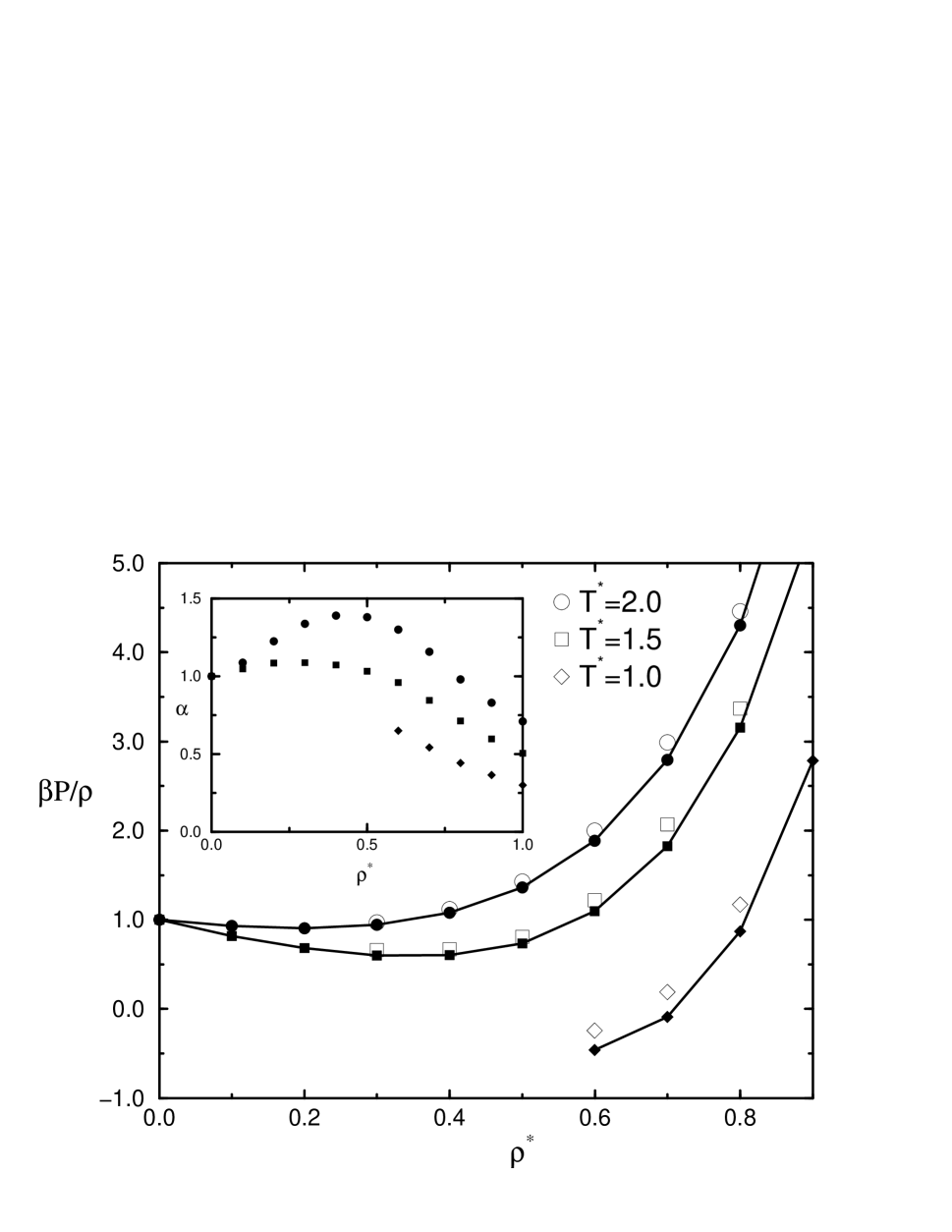
FIG. 1.: Dependence of the compressibility factor $\beta P/\rho$ on density $\rho^{*}$ and temperature $T^{*}$ for the Yukawa fluid. Open symbols represent the results of MD simulations [30] and filled symbols are the predictions of the TIM approximation. Lines are guides to the eye. In the inset: dependence of the self-consistency parameter $\alpha$ in the TIM approach on density $\rho^{*}$ and temperature $T^{*}$.

FIG. 2.: Density correlation functions of the hard core Yukawa fluid. From top to bottom: ($\rho^{*}=0.8,T^{*}=0.9$), ($\rho^{*}=0.4,T^{*}=1.25$), ($\rho^{*}=0.05,T^{*}=1.0$). MC simulations performed in this work. For the sake of clarity, curves have been shifted in the vertical direction.

FIG. 3.: Density correlation functions of the Lennard-Jones fluid. From top to bottom: ($\rho^{*}=0.54,T^{*}=1.35$), ($\rho^{*}=0.45,T^{*}=1.35$), ($\rho^{*}=0.1,T^{*}=1.35$). MD simulations are taken from [31]. For the sake of clarity, curves have been shifted in the vertical direction.

FIG. 4.: Comparison of the shape of $c(r)$ and $t(r)$ for the reference and full Lennard-Jones fluid ($\rho^{*}=0.54,T^{*}=1.35$). This shows the advantage of using $t(r)$ as a variational function instead of $c(r)$ as used in [33].

REFERENCES

- [1] See, e.g., J. P. Hansen and I. R. McDonald, Theory of Simple Liquids, (Academic, London, 1986).
- [2] For an excellent review of Stell’s early work, see G. Stell, in Equilibrium Theory of Classical Fluids, edited by H. L. Frisch and J. L. Lebowitz (W. A. Benjamin, New York, 1964), p.II-171.
- [3] J. K. Percus and G. J. Yevick, Phys. Rev. 110, 1 (1958).
- [4] J. K. Percus, in Equilibrium Theory of Classical Fluids, edited by H. L. Frisch and J. L. Lebowitz (W. A. Benjamin, New York, 1964), p.II-46.
- [5] D. Levesque, Physica 32, 1985 (1966).
- [6] G. Stell, Physica 29, 517 (1963).
- [7] See, e.g., J. S. Hoye and G. Stell, J. Chem. Phys. 67, 439 (1977); J. S. Hoye, J. L. Lebowitz and G. Stell, J. Chem. Phys. 61, 3253 (1974); and references therein.
- [8] W. G. Madden and S. A. Rice, J. Chem. Phys. 72, 4208 (1980).
- [9] F. Lado, Phys. Rev. A 8, 2548 (1973).
- [10] G. Zerah and J. P. Hansen, J. Chem. Phys. 84, 2336 (1986).
- [11] H. S. Kang and F. H. Ree, J. Chem. Phys. 103, 3629 (1995) and references therein.
- [12] J. D. Weeks, D. Chandler, and H. C. Andersen, J. Chem. Phys. 54, 5237 (1971).
- [13] L. S. Ornstein and F. Zernike, Proc. Akad. Sci. (Amsterdam) 17, 793 (1914).
- [14] R. Dickman and G. Stell, Phys. Rev. Lett. 77, 996 (1996); D. Pini, G. Stell and R. Dickman, Phys. Rev. E 57, 2862 (1998).
- [15] See, e.g., L. L. Lee, J. Chem. Phys. 103, 9388 (1995).
- [16] E. Waisman and J. L. Lebowitz, J. Chem. Phys. 56, 3086 (1972).
- [17] For a contrary view, see Ref. [15].
- [18] G. Stell, in Modern Theoretical Chemistry, Vol. 5: Statistical Mechanics, edited by B. J. Berne (Plenum Press, New York, 1977), p. 47.
- [19] H. C. Andersen and D. Chandler, J. Chem. Phys. 57, 1918 (1972).
- [20] D. Duh and A. D.. J. Haymet, J. Chem. Phys. 103, 2625 (1995)
- [21] Y. Rosenfeld and N. W. Ashcroft, Phys. Rev. A 20, 1208 (1979).
- [22] L. L. Lee, J. Chem. Phys. 97, 8606 (1992).
- [23] G. A. Martynov and G. N. Sarkisov, Mol. Phys. 49, 1495 (1983); P. Ballone et. al., Mol. Phys. 59, 275 (1986).
- [24] M. LLano-Restrepo and W. G. Chapman, J. Chem. Phys. 100, 5139 (1994).
- [25] D. Duh and D. Henderson. J. Chem. Phys. 104, 6742 (1996).
- [26] D. Pini, G. Stell and N. B. Wilding, Mol. Phys. 95, 483 (1998); D. Pini, G. Stell and J. S. Hoye, Int. J. Thermophys. 19, 1029 (1998).
- [27] L. Belloni, J. Chem. Phys. 98, 8080 (1993).
- [28] L. Belloni, J. Chem. Phys. 88, 5143 (1988).
- [29] D. Henderson, E. Waisman, J. L. Lebowitz and L. Blum, Mol. Phys. 35, 241 (1978).
- [30] C. Rey, L. J. Gallego and L. E. Gonzalez, J. Chem. Phys. 96, 6984 (1992).
- [31] J. D. Weeks, K. Vollmayr and K. Katsov, Physica (Amsterdam) A 244, 461 (1997).
- [32] W. H. Press, S. A. Teukolsky, W. T. Vettering, B. P. Flannery, Numerical Recipes in C, (Cambridge University Press, 1992).
- [33] A. H. Narten, L. Blum and R. H. Fowler, J. Chem. Phys. 60, 3378 (1974).
- [34] W. Olivares and D. A. McQuarrie, J. Chem. Phys. 65, 3604 (1976).
- [35] M. J. Gillan, Mol. Phys. 38, 1781 (1979); G. Zerah, J. Comput. Phys. 61, 280 (1985).
- [36] Y. Tang and B. C.-Y. Lu, J. Chem. Phys. 103, 7463 (1995).
- [37] D. Chandler, Phys Rev. E 48, 2989 (1993); G. E. Crooks and D. Chandler, Phys. Rev. E 56, 4217 (1997). See also G. Hummer, et al., Proc. Natl. Acad. Sci. 93, 8951 (1996).
- [38] D. E. Sullivan and G. Stell, J. Chem. Phys. 69, 5450 (1978); D. E. Sullivan, D. Levesque, and J. J. Weis, Ibid. 72, 1170 (1980).
- [39] J . D. Weeks, K. Katsov, and K. Vollmayr, Phys. Rev. Lett. 81 4400 (1998); K. Lum, D. Chandler and J. D. Weeks, J. Phys. Chem. B 103, 4570 (1999).