Dynamical Properties of Chiral-Glass Order
in Ceramic High-$T_{c}$ Superconductors

1 Introduction

Due to the enhanced effect of thermal fluctuations, the problem of the phase diagram of cuprate high-$T_{c}$ superconductors becomes highly nontrivial and has attracted much recent interest. For example, in random type-II superconductors under applied magnetic fields, the existence of novel glassy thermodynamic phases distinct from the vortex-liquid phase, such as the Bragg-glass phase ${}^{\hbox{\immediate{\bf{?}})}}$ or the vortex-glass phase ,${}^{\hbox{\immediate{\bf{?}})}}$ have been discussed quite extensively. In zero external field, by contrast, the only thermodynamic phase widely accepted to date is the standard Meissner phase. The $d$-wave nature of high-$T_{c}$ superconductors appears to have little effect on possible thermodynamic phases of bulk high-$T_{c}$ superconductors.

A few years ago, however, it was theoretically proposed that a new zero-field phase, called a chiral-glass phase, might be realized in certain ceramic or granular high-$T_{c}$ superconductors. ${}^{\hbox{\immediate{\bf{?}},\penalty 1000\hskip 0.91003pt plus 0.70004pt minus 0.70004pt{\bf{?}},\penalty 1000\hskip 0.91003pt plus 0.70004pt minus 0.70004pt{\bf{?}})}}$ This state is characterized by the spontaneously broken $Z_{2}$ time-reversal symmetry with keeping the $U(1)$ gauge symmetry. The order parameter is a ‘chirality’, representing the direction of the local loop-supercurrent flowing over grains. In the chiral-glass state, circulation of local loop-supercurrents, spontaneously generated even in zero field, is frozen in time in a spatially random manner. Frustration effect, which arises due to the random distribution of the $\pi$ junctions with the negative Josephson coupling, is essential to realize this phase. In this chiral-glass state, unlike in the Meissner or the vortex-glass state, the phase of the condensate is not ordered, even randomly, on sufficient long length and time scales: The thermodynamic ordering occurs only in the loop-supercurrents, or in the chiralities.

Numerical studies have given support to the existence of such a chiral-glass state both in the presence and absence of screening effect. ${}^{\hbox{\immediate{?},\penalty 1000\hskip 0.91003pt plus 0.70004pt minus 0.70004pt{?},\penalty 1000\hskip 0.91003pt plus 0.70004pt minus 0.70004pt{?},\penalty 1000\hskip 0.91003pt plus 0.70004pt minus 0.70004pt{\bf{?}},\penalty 1000\hskip 0.91003pt plus 0.70004pt minus 0.70004pt{\bf{?}},\penalty 1000\hskip 0.91003pt plus 0.70004pt minus 0.70004pt{\bf{?}},\penalty 1000\hskip 0.91003pt plus 0.70004pt minus 0.70004pt{\bf{?}})}}$ In particular, static critical properties of the chiral-glass transition were studied by means of Monte Carlo (MC) simulations by Kawamura and Li, based on a lattice XY model in which finite screening effect was taken into account. ${}^{\hbox{\immediate{?})}}$ Here note that, since the length unit associated with the intergranular ordering is the mean grain size which is of order micron, screening effect is generally non-negligible. At the chiral-glass transition point, the nonlinear susceptibility was found to diverge with negative sign. Indeed, this prediction was supported by subsequent ac susceptibility measurements on YBa₂Cu₄O₈ ceramics by Matsuura et al. ${}^{\hbox{\immediate{\bf{?}})}}$

The purpose of the present paper is, following the work of ref.5 on the static critical properties, to investigate the dynamical critical properties of the chiral-glass transition, and to discuss its implications to magnetic and transport measurements on high-$T_{c}$ ceramics. A quantity playing a central role in characterizing the dynamical critical properties is the dynamical critical exponent $z$. In order to numerically estimate $z$, we perform dynamical (off-equilibrium) MC simulations on the model previously studied in ref.5. Equipped with both the dynamical and static properties of the model, we present a dynamical scaling analysis for the magnetic response (ac susceptibility) and for the transport property (resistivity). The results are discussed in conjunction with some recent experimental results on high-$T_{c}$ ceramics.

2 Model and Static Properties

In this section, we explain the model and summarize its static critical properties. ${}^{\hbox{\immediate{?})}}$

Regarding a ceramic sample consisting of many superconducting grains as an infinite network of Josephson-junction array, we consider a three-dimensional lattice XY model where the phase variable is coupled to fluctuating magnetic-field variable via a finite self-inductance term. The Hamiltonian is given in the dimensionless form by ${}^{\hbox{\immediate{?},\penalty 1000\hskip 0.91003pt plus 0.70004pt minus 0.70004pt{?},\penalty 1000\hskip 0.91003pt plus 0.70004pt minus 0.70004pt{\bf{?}})}}$

$${\cal H}/J=-\sum_{<ij>}J_{ij}\cos(\theta_{i}-\theta_{j}-A_{ij})+\frac{1}{2{\cal L}}\sum_{p}({\mbox{\boldmath$\nabla$}}\times{\mbox{\boldmath$A$}})^{2},$$ (2.1)

where $\theta_{i}$ is the phase of the condensate of the grain at the $i$-th site of a simple cubic lattice, $A$ the fluctuating gauge potential at each directed link of the lattice, $J_{ij}$ the Josephson coupling between the $i$-th and $j$-th grains, and $J$ is the typical coupling strength. The lattice curl ${\mbox{\boldmath$\nabla$}}\times{\mbox{\boldmath$A$}}$ is the directed sum of $A_{ij}$’s around a plaquette. ${\cal L}$ is the dimensionless self-inductance of a loop (an elementary plaquette), while the mutual inductance between different loops is neglected. The first sum is taken over all nearest-neighbor pairs, while the second sum is taken over all elementary plaquettes on the lattice. Fluctuating variables to be summed over are the phase variable, $\theta_{i}$, at each site and the gauge variable, $A_{ij}$, at each link.

The only source of quenched randomness of the present model lies in the Josephson coupling $J_{ij}$. The $d$-wave nature of high-$T_{c}$ superconductors, which is vitally important in realizing the chiral-glass phase at all, manifests itself in the form of the distribution of the Josephson coupling $J_{ij}$. In unconventional supercondutors with anisotropic pairing symmetry such as $d$-wave superconductors, the Josephson coupling between two superconducting grains could be either positive ($0$-junction) or negative ($\pi$-junction), depending on the relative orientation of the crystal. Frustration arises even in zero external field from the random distribution of both positive and negative couplings, just as in case of spin glasses. The situation here should be contrasted to the well-known vortex-glass (gauge-glass) problem. In the latter, the Hamiotonian lacks the time-reversal symmetry due to external fields, while frustration arises from the external fields, not from $J_{ij}$. In the following, we assume for simplicity $J_{ij}$ to be an independent random variable taking the values $1$ or $-1$ with equal probability ($\pm J$ or binary distribution), each representing the $0$ and $\pi$ junctions.

The dimensionless self-inductance can be related to the bare Josephson penetration depth in units of lattice spacing, $\lambda_{0}$, by

$$\lambda_{0}=1/\sqrt{{\cal L}},$$ (2.2)

Thus, larger inductance corresponds to shorter penetration depth with enhanced effects of screening. In the limit ${\cal L}\rightarrow 0$ (or $\lambda_{0}\rightarrow\infty$), the screening effect becomes negligible and one recovers the standard $XY$ spin-glass Hamiltonian studied in refs.6-9.

Note that the Hamiltonian (2.1) possesses the $Z_{2}$ time-reversal symmetry, in addition to the $U(1)$ gauge symmetry. The chiral-glass state is characterized by the spontaneous breaking of the discrete $Z_{2}$ time-reversal symmetry with preserving the continuous $U(1)$ symmetry. In the standard vortex-glass problem, the Hamiltonian has the $U(1)$ gauge symmetry only, and the ordered state (vortex-glass state) is characterized by the spontaneous breaking of this continuous $U(1)$ gauge symmetry.

We define the local chirality at each plaquette by the gauge-invariant quantity,

$$\kappa_{p}=2^{-3/2}\sum_{<ij>}^{p}J_{ij}\sin(\theta_{i}-\theta_{j}-A_{ij}),$$ (2.3)

where the sum runs over a directed contour along the sides of the plaquette $p$. Physically, the chirality is a half ($\pi$) vortex, being proportional to the loop-supercurrent circulating around a plaquette. If the plaquette $p$ is frustrated, the local chirality $\kappa_{p}$ tends to take a value around $\pm 1$, each sign corresponding to the clockwise or counterclockwise circulating supercurrent, while if the plaquette is unfrustrated, it tends to take a value around zero. Note that the chirality is a pseudoscalar in the sense that it is invariant under the global $U(1)$ gauge transformation, $\theta_{i}\rightarrow\theta_{i}+\Delta\theta,\ A_{ij}\rightarrow A_{ij}$, but changes its sign under the global $Z_{2}$ time-reversal transformation, $\theta_{i}\rightarrow-\theta_{i},\ A_{ij}\rightarrow-A_{ij}$.

Now, according to ref.5, we summarize the static critical properties of the model. The most extensive calculations were performed for the case $\lambda_{0}=1$. The Binder ratio of the chirality was calculated for the $N=L\times L\times L$ lattices with $L=3,4,6,8$, which yielded a clear crossing at a finite temperature. From this observation, the chiral-glass transition temperature was estimated to be $T_{{\rm CG}}=0.286\pm 0.01$ (temperature $T$ is measured in units of $J$). Via a finite-size scaling analysis of the chiral Binder ratio and of the chiral-glass susceptibility, static critical exponents of the chiral-glass transition were estimated to be $\nu=1.3\pm 0.2$ and $\eta=-0.2\pm 0.2$. Other exponents were estimated via the standard scaling relation as $\beta\simeq 0.5$ and $\gamma\simeq 2.9$, etc. Monte Carlo data also clearly showed that the nonlinear susceptibility exhibited a negative divergence at the chiral-glass transition. As mentioned, such a behavior was indeed observed by ac susceptibility measurements. ${}^{\hbox{\immediate{?})}}$

3 Dynamical Critical Properties

In this section, we perform further MC simulations for the model (1.1), aimed at estimating the dynamical critical exponent $z$ associated with the chiral-glass transition. In contrast to the previous simulation of ref.5 on the same model where the system was completely thermalized, we employ here an off-equilibrium Monte Carlo simulation where the system is no longer equilibrated completely. Still, one can extract the exponent associated with equilibrium critical dynamics by controlling the waiting-time dependence of the results. More specifically, we first quench the system from infinite temperature to the chiral-glass transition temperature $T=T_{{\rm CG}}$, and compute the subsequent temporal decay of the chirality autocorrelation function defined by,

$$C_{\kappa}(t_{w},t+t_{w})=\frac{1}{3N}\sum_{p}[<\kappa_{p}(t_{w})\kappa_{p}(t+t_{w})>],$$ (3.1)

where $t$ and $t_{w}$ are the observation and the waiting times, respectively, $<\cdots>$ represents the thermal average, [$\cdots$] represents the configurational average over the bond distribution, and the sum runs over all $3N$ plaquettes on the lattice. As long as one is in the so-called quasi-equilibrium regime, $1<<t<<t_{w}$, the decay of autocorrelations at the critical point should obey the standard power-law,

$$C_{\kappa}(t_{w},t+t_{w})\approx t^{-a},\ \ \ \ a=\frac{1+\eta}{2z},\ \ \ (1<<t<<t_{w}),$$ (3.2)

where the decay exponent $a$ is given by the dynamical exponent $z$ and the static exponent $\eta$ as given above. We have used here the standard scaling relations and put $d=3$. Thus, if one could well control the waiting-time dependence of the data in the quasi-equilibrium regime, one can estimate the equilibrium dynamical exponent from off-equilibrium simulations. Main advantage of this method is that one can deal with relatively large lattices since one need not equilibrate the system completely.

We mainly simulate $L=24$ lattices with free boundary conditions, with varying the waiting time in the range $5,000\leq t_{w}\leq 125,000$. Note that the lattice size studied here, $L=24$, is significantly larger than the maximum lattice size, $L=8$, equilibrated at $T=T_{{\rm CG}}$ in ref.5. Sample average is taken over 10 independent bond realizations. For each realization, we perform four independent runs with using different initial conditions and different sequences of random numbers. In order to check the possible size-dependence, we also take data for $L=16$ lattices.

The Hamiltonian (1.1) still has redundant degrees of freedom associated with local gauge transformations, which are usually fixed by the particular choice of the gauge. While static properties do not depend on the choice of the gauge, it is not entirely clear whether dynamical properties would not depend on it. Thus, we employ two different gauges in our off-equilibrium simulations. One is the ‘temporal gauge’ in which the gauge-independent phase difference $\Psi_{ij}\equiv\theta_{i}-\theta_{j}-A_{ij}$ is taken to be an independent variable, and the other is the Coulomb gauge in which the divergence-free condition $\sum_{\delta}A_{i+\delta}=0$ is imposed at any site $i$. In the temporal gauge, we perform the standard Metropolis updating successively on the $\Psi_{ij}$ variable at each link. In the Coulomb gauge, we perform the Metropolis updating successively, first on the phase variable $\theta_{i}$ at each site, and then on the gauge variables $A_{ij}$ at each plaquette: In the latter procedure, in order to observe the local Coulomb-gauge condition, we propose a type of MC trial which simultaneously shifts the four directed link variables $A_{ij}$ around a plaquette by the same amount $A_{ij}\rightarrow A_{ij}+\delta A$. We put $\lambda_{0}=1$ (or ${\cal L}=1$), and set the temperature to the chiral-glass transition temperature for this inductance, $T=T_{{\rm CG}}=0.286$, which was determined by the previous equilibrium simulation. ${}^{\hbox{\immediate{?})}}$

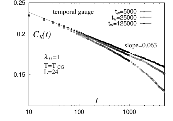
Fig.  1: A log-log plot of the observation time dependence of the chiral autocorrelation function calculated in the temporal gauge for several waiting times. The bare penetration depth is $\lambda_{0}=1$, and the temperature is set at the chiral-glass transition temperature, $T=0.286$. The lattice size is $L=24$.

In Fig.1, we show on a log-log plot the MC time dependence of the chirality autocorrelation function at $T=T_{{\rm CG}}$ calculated in the temporal gauge. As can be seen from the figure, the short-time data for longer waiting times tend to lie on a common straight line with a slope equal to $a=0.063\pm 0.006$.

In order to check consistency, we also calculate the spin-glass-type chirality autocorrelation function defined by

$$q^{(2)}_{\kappa}(t_{w},t+t_{w})=\left[\left<\left(\frac{1}{3N}\sum_{p}\kappa_{p}(t_{w})\kappa_{p}(t+t_{w})\right)^{2}\right>\right].$$ (3.3)

At $T=T_{{\rm CG}}$, $q^{(2)}_{\kappa}$ in the quasi-equilibrium regime is expected to decay asymptotically as

$$q^{(2)}_{\kappa}(t_{w},t+t_{w})\approx t^{-2a},\ \ \ (1<<t<<t_{w}).$$ (3.4)

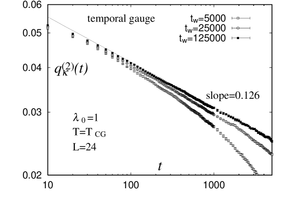
Fig.  2: A log-log plot of the observation time dependence of the spin-glass-type chiral autocorrelation function calculated in the temporal gauge for several waiting times. The bare penetration depth is $\lambda_{0}=1$, and the temperature is set at the chiral-glass transition temperature, $T=0.286$. The lattice size is $L=24$.

In Fig.2, $q^{(2)}_{\kappa}$ calculated in the temporal gauge is shown, which gives a slope $2a=0.126\pm 0.012$, consistently with the $a$ value obtained above from $C_{\kappa}$. We note that a similar analysis of $C_{\kappa}$ and $q^{(2)}_{\kappa}$ made for smaller $L=16$ lattices has given the $a$ value close to this indicating that the finite-size effect is negligible here. Combining the estimate of $a$ with the previous estimate of $\eta=-0.2\pm 0.2$, the dynamical exponent $z$ is obtained as $z=6.3\pm 1.7$.

To check the possible dependence on the choice of the gauge, we repeat a similar calculation also in the Coulomb gauge. As an example, the chiral autocorrelation function $C_{\kappa}$ calculated in the Coulomb gauge is shown in Fig.3. The obtained estimate $a=0.058\pm 0.006$ turns out to be slightly smaller than, but rather close to the value obtained in the temporal gauge.

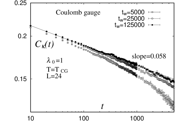
Fig.  3: A log-log plot of the observation time dependence of the chiral autocorrelation function calculated in the Coulomb gauge for several waiting times. The bare penetration depth is $\lambda_{0}=1$, and the temperature is set to the chiral-glass transition temperature, $T=0.286$. The lattice size is $L=24$.

One remark is to be added here. In the present simulation, we have implemented the standard Metropolis dynamics for the Hamiltonian in its original form, i.e. in the phase representation. Instead, one can also employ the vortex representation of the same Hamiltonian, i.e., the dual version. In contrast to the static critical properties, the dynamic critical properties may well depend on which representation is used. In fact, in the numerical study of another model, e.g., the three-dimensional gauge-glass model, the phase and vortex representations gave somewhat different $z$ values, namely, $z\simeq 3.1$ in the vortex (dual) representation ${}^{\hbox{\immediate{?})}}$ which was considerably smaller than $z=4.7\pm 0.7$ obtained in the phase representation. ${}^{\hbox{\immediate{\bf{?}})}}$ Hence, in the present model, there still remains a possibility that the vortex representation yields the $z$ value somewhat different from our present estimate obtained in the phase representation. Unfortunately, we do not know at present which representation is more appropriate in describing the real dynamics of experimental systems.

4 Dynamical Scaling Analysis

In this section, on the basis of the result obtained in the previous section, we proceed to the dynamical scaling analysis both for the magnetic response and for the transport.

4.1 Magnetic response

First, we discuss the dynamical magnetic response near the chiral-glass transition, in particular the ac susceptibilities such as $\chi^{\prime\prime}(\omega)$ and $\chi^{\prime}(\omega)$. Dynamical scaling analysis yields,

$$\chi^{\prime\prime}(\omega,T)\approx\omega^{\frac{\beta}{z\nu}}\bar{\chi}^{\prime\prime}(\frac{\omega}{t^{z\nu}})\approx\omega^{\frac{1+\eta}{2z}}\bar{\chi}^{\prime\prime}(\frac{\omega}{t^{z\nu}}),$$ (4.1)

and similarly for $\chi^{\prime}(\omega,T)$, where $z$ is the dynamical chiral-glass exponent determined above as $z=6.3\pm 1.7$. Other exponents have been estimated numerically as $z\nu\simeq 8.2$, $\beta\simeq 0.5$ and $\eta\simeq-0.2$ etc.

Experimentally, dynamic scaling analyses were made for the zero-field $\chi^{\prime\prime}$ data of some high-T_c ceramic superconductors such as LSCO ${}^{\hbox{\immediate{\bf{?}})}}$ and YBCO. ${}^{\hbox{\immediate{\bf{?}})}}$ In particular, Deguchi et al recently performed a dynamic scaling analysis of the zero-field $\chi^{\prime\prime}$ data of YBa₂Cu₄O₈ ceramics at its intergranular transition point. ${}^{\hbox{\immediate{?})}}$ In this sample, the intergranular transition occurs at a temperature much below the intragranular transition temperature, the latter being the bulk superconducting transition temperature of single-crystal YBa₂Cu₄O₈. Since the effect of intragranular transition is well separated from the intergranular one, the sample is well suited to the study of intergranular transition of interest here. Deguchi et al then found a reasonable scaling fit of the data, with the choice of critical exponents, $z\nu\simeq 8$ and $\beta\simeq 0.57$, the values fairly close to our present estimates $z\nu\simeq 8.2$ and $\beta\simeq 0.5$.

4.2 Transport property

As mentioned, in the chiral-glass state, the $U(1)$ gauge symmetry is not broken, even randomly, in the strict sense. This means that the phase of the condensate, $\theta$, remains disordered on sufficiently long length and time scales. Free motion of integer vortex lines is still possible in the chiral-glass state where chiralities (half-vortices) sitting at frustrated plaquettes are frozen. A schematic picture showing such free motion of integer vortex-line excitations in the background of frozen pattern of chiralities is given in Fig.4. One can see that free motion of integer-vortex lines of either sign is possible without seriously destroying the freezing pattern of chiralities in the background. In order to destroy the chiral-glass ordering in the background, a chiral domain-wall-type excitation is necessary, which would be responsible for the chiral-glass transition at $T=T_{{\rm CG}}$. Thus, the chiral-glass state should not be a true superconductor, with a small but nonvanishing linear resistivity $\rho_{L}$ even at and below $T_{{\rm CG}}$. Rough estimates of the residual $\rho_{L}$ was given in ref.5b.

Fig.  4: Two-dimensional segment of the lattice showing thermally-activated integer vortex lines with vorticity $\pm 1$, wandering in the background of a frozen pattern of chiralities in the chiral-glass state. Plus (+) and minus ($-$) chirality can be viewed as half-vortices with vorticity $\pm 1/2$ at frustrated plaquettes, while unfrustrated plaquettes are frozen into the zero-chirality ($0$) state. If one looks at a given frustrated plaquette frozen into the + chirality (or vorticity $+1/2$) state, for example, its vorticity occasionally becomes $+3/2$ or $-1/2$ when the thermally-activated integer vortex line of either sign, +1 or -1, passes this plaquette. Still, the long-time average of the vorticity at this plaquette is equal to $+1/2$, showing that the free motion of integer vortex lines is compatible with the long-range chiral-glass order.

Now, based on such a physical picture, we try to perform a dynamical scaling analysis of the transport property of ceramic high-$T_{c}$ superconductors near the chiral-glass transition. Suppose that, under the external current of density $j$, there occurs a voltage drop, or electric field of intensity $E$. The above physical picture suggests that the voltage drop comes from the two nearly independent sources: One from the motion of integer vortex lines, $E_{v}$, and the other from the motion of chiral domain walls, $E_{\kappa}$. Namely, one has

$$E(j,T)=E_{v}(j,T)+E_{\kappa}(j,T).$$ (4.2)

The first part is expected to be essentially a regular part, while the second part should obey the dynamic scaling law associated with the chiral-glass transition, i.e.,

$$E_{\kappa}\approx\mid t\mid^{(z+1)\nu}\bar{E}_{\kappa}(j/\mid t\mid^{2\nu}),$$ (4.3)

where $t$ is a reduced temperature $t\equiv(T-T_{{\rm CG}})/T_{{\rm CG}}$, and the spatial dimension has been set equal to $d=3$. Standard analysis yields the following asymptotic behaviors of the scaling function, ^2b

$$\bar{E}_{\kappa}(x)\approx\left\{\begin{array}[]{ll}ax,&(t>0),\\ a^{\prime}\exp[-bx^{-\mu}],&(t<0),\end{array}\right.\ \ \ \ \ \ {\rm as}\ x\rightarrow 0,$$ (4.4)

where $a$, $a^{\prime}$ and $b$ are positive constants, and $\mu$ is an exponent describing the chirality dynamics in the chiral-glass state.

The linear resistivity $\rho_{L}$ can also be written as a sum of the two nearly independent contributions,

$$\rho_{L}\equiv\left.\frac{{\rm d}E}{{\rm d}j}\right|_{j=0}=\rho_{L,v}+\rho_{L,\kappa}.$$ (4.5)

At and near the chiral-glass transition point $T=T_{{\rm CG}}$, the first term $\rho_{L,v}(T)$ stays finite without prominent anomaly at $T=T_{{\rm CG}}$,

$$\rho_{L,v}(T)\approx\rho_{0}+ct+\cdots,$$ (4.6)

while the second term $\rho_{L,\kappa}(T)$ exhibits a singular behavior associated with the chiral-glass transition, i.e., one has from eq.(4.3)

$$\rho_{L,\kappa}(T)\approx\left\{\begin{array}[]{ll}0,&(t<0),\\ c^{\prime}t^{(z-1)\nu},&(t>0).\end{array}\right.$$ (4.7)

Since $(z-1)\nu\simeq 6.9$ is a large positive number, the second term of eq.(4.5) vanishes toward $T_{{\rm CG}}$ rather sharply, and the behavior of $\rho_{L}$ is dominated by the regular term $\rho_{L,v}(T)$. Thus, the total linear resistivity remains finite at $T=T_{{\rm CG}}$. The singular behavior borne by $\rho_{L,\kappa}(T)$ would be masked by the regular term and hardly detectable experimentally.

By contrast, a stronger anomaly could arise in the nonlinear resistivity $\rho_{NL}$. If one considers the lowest-order nontrivial one, it is again a sum of the two nearly independent contributions,

$$\rho_{NL}\equiv\frac{1}{6}\left.\frac{{\rm d}^{3}E}{{\rm d}j^{3}}\right|_{j=0}=\rho_{NL,v}+\rho_{NL,\kappa}.$$ (4.8)

The first part is essentially a regular term, while the second part can be written from eq.(4.3) in the scaling form,

$$\rho_{NL,\kappa}(T)\approx\left\{\begin{array}[]{ll}0,&(t<0),\\ c^{\prime\prime}t^{(z-5)\nu},&(t>0).\end{array}\right.$$ (4.9)

Thus, the nonlinear resistivity $\rho_{NL}(T)$ shows a stronger anomaly than the linear resistivity $\rho_{L}(T)$. In particular, if $z$ is smaller than five, the nonlinear resistivity $\rho_{NL}(T)$ exhibits a positive divergence at $T=T_{{\rm CG}}$. Then, the chiral-glass transition, even though it hardly manifests itself in the linear resistivity, should clearly be detectable as a strong anomaly in the nonlinear resistivity. Although our present best estimate obtained in the phase representation, $z=6.3\pm 1.7$, comes slightly larger than five, it is not incompatible with a value smaller than five within the errors. Furthermore, as discussed at the end of §4, $z$ may possibly take a smaller value in the vortex representation than in the phase representation. Taking account of these uncertainties, there still exists a possibility that the value of $z$ relevant here is smaller than five, and the nonlinear resistivity exhibits a real divergence at $T=T_{{\rm CG}}$.

Recently, Yamao et al measured via ac technique the linear and nonlinear resistivities of YBa₂Cu₄O₈ ceramics in zero external field. ${}^{\hbox{\immediate{\bf{?}})}}$ They observed a divergent behavior in the nonlinear resistivity just at the temperature where the nonlinear magnetic susceptibility showed a negative divergence and where the magnetic remanence set in. Meanwhile, the linear resistivity remained finite without any appreciable anomaly there. Such behaviors are hard to understand if one regards the observed transition as the standard Meissner or the vortex-glass transition. Recall that the linear resistivity should vanish in the Meissner or the vortex-glass transition, which is clearly at odds with the experimental finding of ref.15. In contrast, the experimental result seems fully compatible with the chiral-glass picture discussed in this paper.

5 Summary

The dynamical critical properties of the chiral-glass ordering were studied by means of Monte Carlo simulations and the dynamical scaling analysis. We emphasize that the chiral-glass state is a new zero-field phase of superconductors, being first made possible by the anisotropic nature of the pairing symmetry of cuprate superconductors. In particular, we have shown that recent magnetic and transport measurements on YBCO high-$T_{c}$ ceramics are consistent with the chiral-glass picture.

While in this paper we have concentrated ourselves on the equilibrium dynamical critical properties at and near the chiral-glass transition, complete thermalization is practically impossible deep into the chiral-glass state in real ceramics. There, interesting off-equilibrium phenomena similar to those observed in spin glasses, such as aging effects and memory phenomena, are certainly expected. For example, Papadopoulou et al recently observed an aging effect in certain ceramic BSCCO sample at very weak fields,  ${}^{\hbox{\immediate{\bf{?}})}}$ though the connection to the possible chiral-glass order was not necessarily clear yet. For the future, further theoretical and experimental studies of off-equilibrium dynamical properties of the chiral-glass ordered state would be of much interest.

References

- [1] T. Nattermann: Phys. Rev. Lett. 64 (1990) 2454; T. Giamarchi and P. LeDoussal: Phys. Rev. Lett. 72 (1994) 1530; T. Emig, S. Bogner and T. Nattermann: Phys. Rev. Lett. 83 (1999) 400.
- [2] (a) M.P.A. Fisher: Phys. Rev. Lett. 62 (1989) 1415; (b) D.S. Fisher, M.P.A. Fisher and D.A. Huse: Phys. Rev. B43 (1991) 130.
- [3] H. Kawamura: J. Phys. Soc. Jpn. 64 (1995) 711.
- [4] H. Kawamura and M.S. Li: Phys. Rev. B53 (1996) 619.
- [5] (a) H. Kawamura and M.S. Li: Phys. Rev. Lett. 78 (1997) 1556; (b) J. Phys. Soc. Jpn. 66 (1997) 2111.
- [6] H. Kawamura and M. Tanemura: J. Phys. Soc. Jpn. 60 (1991) 608.
- [7] H. Kawamura: Phys. Rev. B51 (1995) 12398.
- [8] C. Wengel and A.P. Young: Phys. Rev. B56, 5918 (1997).
- [9] J. Maucourt and D. R. Grempel: Phys. Rev. Lett. 80 (1998) 770.
- [10] M. Matsuura, M. Kawachi, K. Miyoshi, M. Hagiwara and K. koyama: J. Phys. Soc. Jpn. 65 (1995) 4540.
- [11] D. Domínguez, E.A. Jagla and C.A. Balseiro: Phys. Rev. Lett. 72 (1994) 2773.
- [12] J.D. Reger, T.A. Tokuyasu, A.P. Young and M.P.A. Fihser: Phys. Rev. B44 (1991) 7147.
- [13] L. Leylekian, M. Ocio and J. Hammann: Physica C185-189 (1991) 2243; Physica B194-196 (1994) 1865.
- [14] H. Deguchi, T. Hongo, K. Noda, S. Takagi, K. Koyama and M. Matsuura: AIP Conf. Proceeding of 8th Tohwa University International Symposium, ed. by M. Tokuyama and I. Oppenheim, (1999) 539.
- [15] T. Yamao, M. Hagiwara, K. Koyama and M. Matsuura: J. Phys. Soc. Jpn. 68 (1999) 871.
- [16] E.L. Papadopoulou, P. Nordblad, P. Svedlindh, R. Schöneberger and R. Gross, Phys. Rev. Lett. 82 (1999) 173.