Quantum impurity dynamics in two-dimensional antiferromagnets and superconductors

Abstract

We present the universal theory of arbitrary, localized impurities in a confining paramagnetic state of two-dimensional antiferromagnets with global SU(2) spin symmetry. The energy gap of the host antiferromagnet to spin-1 excitations, $\Delta$, is assumed to be significantly smaller than a typical nearest neighbor exchange. In the absence of impurities, it was argued in earlier work (Chubukov et al. Phys. Rev. B 49, 11919 (1994)) that the low-temperature quantum dynamics is universally and completely determined by the values of $\Delta$ and a spin-wave velocity $c$. Here we establish the remarkable fact that no additional parameters are necessary for an antiferromagnet with a dilute concentration of impurities, $n_{\text{imp}}$—each impurity is completely characterized by a integer/half-odd-integer valued spin, $S$, which measures the net uncompensated Berry phase due to spin precession in its vicinity. We compute the impurity-induced damping of the spin-1 collective mode of the antiferromagnet: the damping occurs on an energy scale $\Gamma=n_{\text{imp}}(\hbar c)^{2}/\Delta$, and we predict a universal, asymmetric lineshape for the collective mode peak. We argue that, under suitable conditions, our results apply unchanged (or in some cases, with minor modifications) to d-wave superconductors, and compare them to recent neutron scattering experiments on ${\rm Y}{\rm Ba}_{2}{\rm Cu}_{3}{\rm O}_{7}$ by Fong et al. (Phys. Rev. Lett. 82, 1939 (1999)). We also describe the universal evolution of numerous measurable correlations as the host antiferromagnet undergoes a quantum phase transition to a Néel ordered state.

I Introduction

The study of two-dimensional doped antiferromagnets is a central subject in quantum many-body theory. A plethora of interesting quantum ground states and quantum phase transitions appear possible, and the results have important experimental applications to the cuprate high temperature superconductors and other layered transition metal compounds. However the zoo of possibilities contributes to the complexity of the problem, and a widely accepted quantitative theory has not yet appeared.

This paper will present a detailed quantum theory of some simpler realizations of doped antiferromagnets. We will consider situations in which it is possible to neglect the coupling between the spin and charge degrees of freedom and consider a theory of the spin excitations alone. More specifically, we have in mind the following physical systems, which are the focus of intense current experimental interest:
(A) Quasi-two dimensional ‘spin gap’ insulators exp1 ; exp2 ; exp3 ; exp4 ; exp5 like ${\rm SrCu}_{2}{\rm O}_{3}$, ${\rm CuGeO}_{3}$ or ${\rm NaV}_{2}{\rm O}_{5}$ in which a small fraction of the magnetic transition metal ions (Cu or V) are replaced by non-magnetic ions by doping with Zn or Li. These insulators have a gap to both charge and spin excitations, but the spin gap is significantly smaller than the charge gap, validating a theory of the spin excitations alone. Moreover, additional low energy spin excitations are created in the vicinity of the dopant ions while charge fluctuations are strongly suppressed everywhere.
(B) High temperature superconductors like ${\rm Y}{\rm Ba}_{2}{\rm Cu}_{3}{\rm O}_{7}$ in which a small fraction of Cu has been replaced by non-magnetic Zn or Li fink ; alloul ; alloul2 ; tomo ; alloul2a ; sisson ; mendels ; alloul3 ; julien ; keimer ; seamus . A major fraction of the spectral weight of the spin excitiations near momentum ${\bf Q}=(\pi,\pi)$ resides in a spin-1 ‘resonance peak’ at energy $\Delta=40\text{meV}$ rossat1 ; mook ; tony3 ; bourges ; he . We present here a theory for the changes in this peak due to the doping by non-magnetic ions. It may appear surprising that we are able to model this phenomenon by a theory of the spin excitations alone, but we shall describe how this is possible: under suitable conditions, the coupling between the bosonic spin-1 mode responsible for the resonance peak, and the spin-1/2 fermionic, Bogoliubov quasiparticles of the d-wave superconductor is weak and, in a sense we will make precise, irrelevant. (The alternative case in which the coupling to the quasiparticles is relevant is discussed in Appendix A— here we find that qualitative features of the theory and the structure of all the scaling forms remain unchanged, and there are only quantitative changes to scaling functions.) We will obtain a universal expression for the energy scale over which the resonance peak is broadened by non-magnetic ions, with the result depending only upon known bulk parameters. We also predict an unusual asymmetric lineshape for the broadened peak at low temperatures, and it would be interesting to test this in future experiments.

Related questions have been addressed in some earlier work. The impurity-induced damping of bulk excitations of an antiferromagnet was addressed in Ref. harris, : however, their analysis was restricted to the doublet spin-wave excitations of an ordered Néel state well away from any quantum critical point; our focus here is on the triplet excitations in the paramagnetic phase. A weak-coupling analysis of the effect of Zn impurities on the spin fluctuation spectrum of a traditional BCS superconductor was considered in Ref. bulut, .

An elementary introduction and a summary of our results, mainly for the uniform spin susceptibility, have appeared previously Science .

Although our results apply to disparate physical systems, they are unified by their reliance on a simple, new quantum field theory. We find it convenient to introduce this field theory at the outset, and will attempt to keep the discussion here self-contained and accessible to experimentalists. The discussion in this introduction will be divided into four subsections: Section I.1 will review the quantum field theory for the host antiferromagnet, Section I.2 will introduce the new quantum field theory of the impurity problem, our main results will be described in Section I.3, while the outline of the remainder of the paper appears in Section I.4.

I.1 Host antiferromagnet

We shall assume that the spin fluctuations in the host antiferromagnet, prior to doping by the Zn or Li ions, are described by the following O(3)-symmetric quantum theory book of a three-component vector field $\phi_{\alpha}(x,\tau)$ ($\alpha=1\ldots 3$)

$$\quad Z_{\text{b}}^{\prime}=\int{\cal D}\phi_{\alpha}(x,\tau)\exp\left(-{\cal S}_{\text{b}}^{\prime}\right)$$

$$\mathcal{S}_{\text{b}}^{\prime}=\int d^{2}x\int_{0}^{\beta}d\tau\bigg{[}\frac{1}{2}\left((\partial_{\tau}\phi_{\alpha})^{2}+c_{1}^{2}(\partial_{x_{1}}\phi_{\alpha})^{2}\right.$$

$$\qquad\left.+c_{2}^{2}(\partial_{x_{2}}\phi_{\alpha})^{2}+s\phi_{\alpha}^{2}\right)+\frac{g_{0}}{4!}\left(\phi_{\alpha}^{2}\right)^{2}\bigg{]}.$$ (1)

Here repeated indices $\alpha$ are implicitly summed over, $x=(x_{1},x_{2})$ is the two-dimensional spatial co-ordinate, $\tau$ is imaginary time,

$$\beta=\frac{\hbar}{k_{B}T},$$ (2)

and $T$ is the temperature. The field $\phi_{\alpha}(x,\tau)$ represents the instantaneous, local orientation and magnitude of the antiferromagnetic order parameter. So in applications to ${\rm Y}{\rm Ba}_{2}{\rm Cu}_{3}{\rm O}_{7}$, $\phi_{\alpha}$ represents the amplitude of spin fluctuations near wavevector ${\bf Q}=(\pi,\pi)$. More generally, $\phi_{\alpha}$ can represent collinear spin fluctuations at any commensurate wavevector, apart from wavevector $(0,0)$. So states with significant ferromagnetic fluctuations are excluded, as are spiral states (like those on the triangular lattice antiferromagnet) which have non-collinear spin order. Incommensurate, but collinear, spin correlations can be treated by a simple extension of the theory we consider here - this is discussed briefly in Appendix B.

The quantum dynamics of $\phi_{\alpha}$ is realized by the second-order time derivative term in $\mathcal{S}_{\text{b}}^{\prime}$; we have rescaled the $\phi_{\alpha}$ field to make the co-efficient of this term unity. Notice that there is no first-order Berry phase term, as is found in the path integral of a single spin: these are believed to efficiently average to zero on the scale of a few lattice spacings, because the orientation of the spins oscillates rapidly in the antiferromagnet. In one-dimensional antiferromagnets, this lattice scale cancellation is not quite perfect, and a topological ‘$\theta$-term’ does survive book ; however no such terms appear in two dimensions–the fate of the Berry phases in the host antiferromagnet has been discussed at length elsewhere book ; rs1 ; CSY , and will not be important for our purposes here.

The spatial propagation of the spin excitations is associated with the two spatial gradient terms, and we have allowed for two distinct spin-wave velocities, $c_{1}$, $c_{2}$, for propagation in the $x_{1}$ and $x_{2}$ directions. Such anisotropies are present in the coupled ‘spin-ladder’ systems like ${\rm SrCu}_{2}{\rm O}_{3}$. However, a simple redefinition of spatial co-ordinates

$$x_{1}\rightarrow\left(\frac{c_{1}}{c_{2}}\right)^{1/2}x_{1}\quad;\quad x_{2}\rightarrow\left(\frac{c_{2}}{c_{1}}\right)^{1/2}x_{2},$$ (3)

allows us to scale away the anisotropy, and we shall assume this has been done in our subsequent discussion, unless explicitly stated otherwise. The resulting partition function has the form

$$Z_{\text{b}}= \int{\cal D}\phi_{\alpha}(x,\tau)\exp\left(-\mathcal{S}_{\text{b}}\right)$$

$$\mathcal{S}_{\text{b}}=\int d^{d}x\int_{0}^{\beta}d\tau \bigg{[}\frac{1}{2}\left((\partial_{\tau}\phi_{\alpha})^{2}+c^{2}(\nabla_{x}\phi_{\alpha})^{2}+s\phi_{\alpha}^{2}\right)$$ (4)

$$\qquad+\frac{g_{0}}{4!}\left(\phi_{\alpha}^{2}\right)^{2}\bigg{]},$$

where

$$c=(c_{1}c_{2})^{1/2}.$$ (5)

We have also generalized the action to $d$ spatial dimensions for future convenience.

The most important property of $\mathcal{S}_{\text{b}}$ is that it exhibits a phase transition as a function of the coupling $s$ book . For $s$ smaller than a critical value $s_{c}$, the ground state has magnetic Néel order and spin rotation invariance is broken because $\langle\phi_{\alpha}\rangle\neq 0$. For $s>s_{c}$, spin rotation invariance is restored, and the ground state is a quantum paramagnet with a spin gap. The properties of this phase transition in $\mathcal{S}_{\text{b}}$ are well understood, and we review a few salient facts. The Néel state of $\mathcal{S}_{\text{b}}^{\prime}$ is characterized by two spin stiffnesses, $\rho_{s1}$, $\rho_{s2}$, which measure the energy cost to slow twists in the direction of the Néel order in the 1,2 directions respectively (more precisely, a uniform twist by an angle $\theta$ over a length $L$ in the $i$ direction costs energy $(\rho_{si}/2)(\theta/L)^{2}$ per unit volume; note that $\rho_{si}$ has the dimension of energy in $d=2$). These stiffnesses are related by

$$\frac{\rho_{s1}}{\rho_{s2}}=\frac{c_{1}^{2}}{c_{2}^{2}}.$$ (6)

For the isotropic model $\mathcal{S}_{\text{b}}$ we have a single spin stiffness

$$\rho_{s}=\left(\rho_{s1}\rho_{s2}\right)^{1/2}.$$ (7)

As $s$ approaches $s_{c}$ from below, the velocities $c_{1}$ and $c_{2}$ remain constant, while

$$\rho_{s}\sim(s_{c}-s)^{(d-1)\nu}.$$ (8)

where $\nu$ is a known exponent. The quantum paramagnet for $s>s_{c}$ is characterized by its spin gap $\Delta$, and this vanishes as $s$ approaches $s_{c}$ from above as

$$\Delta\sim(s-s_{c})^{\nu}.$$ (9)

As has been discussed at length elsewhere CSY ; book , provided $|s-s_{c}|$ and $T$ are not too large, the energy scales $\Delta$ and $\rho_{s}$, and the velocities $c_{1}$, $c_{2}$, are sufficient to completely characterize the quantum dynamics of a $d=2$ antiferromagnet; there is no need to have an additional parameter determining the strength of the quartic non-linearity $g_{0}$ because it reaches a universal value, determined by the zero of a renormalization group beta function, near the critical point. The present paper will establish the remarkable fact that no additional parameters are needed to characterize the spin dynamics in the presence of a dilute concentration of impurities. As we shall specify more explicitly below, we only need to know the concentration of impurities, $n_{\text{imp}}$, and for each impurity a spin $S$, which is integer or half-odd-integer; the value of $S$ can usually be determined, a priori, by simple arguments based upon gross features of the impurity configuration.

Many simple, physically relevant, lattice antiferromagnets can be explicitly shown to have a quantum phase transition described by $\mathcal{S}_{\text{b}}$. One of the most transparent is the coupled-ladder antiferromagnet, which has been much studied in recent work katoh ; imada ; kotov1 ; twor ; kotov2 ; lt . We will consider such a model in Section III.1: the relationship to $\mathcal{S}_{\text{b}}$ will emerge naturally, and we will also be able to relate parameters in $\mathcal{S}_{\text{b}}$ to microscopic couplings. Other models include the double-layer antiferromagnet hida ; mm ; sand ; gelfand ; troyerss , the antiferromagnet on the 1/5-depleted square lattice troyer , and the square lattice antiferromagnet with frustration rs2 ; kotov3 ; rrps ; kotov4 : our results will also apply to such antiferromagnets.

The reader might wonder why we are placing an emphasis on the quantum phase transition in $\mathcal{S}_{\text{b}}$, while most experiments on Zn or Li doping have taken place in an antiferromagnet or superconductor with a well-defined spin gap. The reason is that the spin gap, $\Delta$, is often significantly smaller than the microscopic exchange interactions, $J$. Under such circumstances, it is a poor approximation to model the spin gap phase in terms on tightly bound singlet pairs of electrons. Rather, the smallness of the gap indicates that there is an appreciable spin correlation length and significant resonance between different pairings of singlet bonds. The approach we advocate to describe such a fluctuating singlet state is to find a quantum critical point to an ordered Néel state somewhere in parameter space, and to expand away from it back into the spin gap phase. It is not necessary that the quantum critical point be experimentally accessible for such an approach to be valid: all that is required is that it be near a physically accessible point. The value of expanding away from the quantum critical point is that detailed dynamical information can be obtained in a controlled manner, dependent only upon a few known parameters.

I.2 Quantum impurities

We now introduce arbitrary localized impurities at a set of random locations $\{r\}$ with a density $n_{\text{imp}}$ per unit volume. We place essentially no restrictions on the manner in which each impurity deforms the host antiferromagnet, provided the deformations are localized, immobile, well separated from each other, and preserve global SU(2) spin symmetry. As we argue below, each impurity will be characterized only by a single integer/half-odd-integer, $S_{r}$, which measures the net imbalance of Berry phase in the vicinity of the impurity; all other characteristics of the impurity will be shown to be strongly irrelevant. We mentioned the essentially complete cancellations of Berry phases in the host antiferromagnet earlier in Section I.1; this cancellation can be disrupted in the presence of an impurity SY ; sigrist1 , and it is only this disruption which will be important in the low energy limit. For instance, a single Zn or Li impurity introduces one additional spin on one sublattice than on the other, and so in a host spin-1/2 antiferromagnet such an impurity will have $S_{r}=1/2$. As another example, consider a ferromagnetic rung bond in a spin-1/2 coupled ladder antiferromagnet: the two spins on the ends of the rung will be oriented parallel to each other and so their Berry phases will add rather than cancel, leading to $S_{r}=1$.

The above criteria determining $S_{r}$ are qualitative, but we can make them more precise. Place the host antiferromagnet in the quantum paramagnetic phase ($s>s_{c}$) and measure the response to a uniform magnetic field. In the absence of impurities, the total linear susceptibility of the antiferromagnet, $\chi$, can be written as $\chi=(g\mu_{B})^{2}\mathcal{A}\chi_{\text{b}}$, where $\mathcal{A}$ is the total area of the antiferromagnet, $g$ is the gyromagnetic ratio, $\mu_{B}$ is the Bohr magneton, and $\chi_{\text{b}}$ is the response per unit area. As $T\rightarrow 0$, the response is exponentially small due to the presence of a spin gap, $\Delta$; a simple argument summing over a dilute gas of thermally excited spin-1 particles shows that book

$$\chi_{\text{b}}(T\rightarrow 0)=\frac{\Delta}{\pi\hbar^{2}c^{2}}e^{-\Delta/k_{B}T}.$$ (10)

Now let us add a very small concentration of impurities. The response $\chi$ is modified to

$$\chi=(g\mu_{B})^{2}\big{[}\mathcal{A}\chi_{\text{b}}+\chi_{\text{imp}}\big{]}\,.$$ (11)

Provided the impurities are dilute enough that they do not interact with each other, then $\chi_{\text{imp}}$ must take the following form at low $T$:

$$\chi_{\text{imp}}=\sum_{r}\frac{S_{r}(S_{r}+1)}{3k_{B}T}.$$ (12)

We will take the values of $S_{r}$ which appear in such an observation of $\chi_{\text{imp}}$ as the definitions of impurity spins $S_{r}$ at the site $r$: they will necessarily be integers/half-odd-integers when the host antiferromagnet has a spin gap. It is important to note that for any fixed $n_{\text{imp}}$, there is an exponentially small temperature below which the impurities do interact with each other, and (12) is no longer valid: we have assumed that $T$ is above such a temperature in determining the $S_{r}$. However, once the $S_{r}$ have been obtained, our quantum theory below will also apply in the interacting impurity regime.

We now describe the modifications to the bulk action $\mathcal{S}_{\text{b}}$ by the quantum impurities with spin $S_{r}$ at sites $\{r\}$. The divergent Curie susceptibility in (12) is a consequence of the free rotation of the impurity spin in spin space. Let us denote the instantaneous orientation of the impurity spin at $r$ by the unit vector $n_{r\alpha}(\tau)$, where $\alpha=1\ldots 3$ and $\sum_{\alpha}n_{r\alpha}^{2}(\tau)=1$. Then the field theory of the quantum impurity problem is

$$Z=\int{\cal D}\phi_{\alpha}(x,\tau){\cal D}n_{r\alpha}(\tau)\delta\left(n_{r\alpha}^{2}-1\right)\exp\left(-\mathcal{S}_{\text{b}}-\mathcal{S}_{\text{imp}}\right)$$

$$\mathcal{S}_{\text{imp}}=\sum_{r}\int_{0}^{\beta}d\tau\bigg{[}iS_{r}A_{\alpha}(n_{r})\frac{dn_{r\alpha}(\tau)}{d\tau}$$

$$~{}~{}~{}~{}~{}~{}~{}~{}~{}~{}~{}~{}~{}~{}~{}~{}~{}~{}~{}~{}~{}~{}~{}~{}~{}-\gamma_{0r}S_{r}\phi_{\alpha}(x=r,\tau)n_{r\alpha}(\tau)\bigg{]}.$$ (13)

The first term in $\mathcal{S}_{\text{imp}}$ is uncompensated Berry phase of the impurity at site $r$: the spin $S_{r}$ is precisely that appearing in (12) and $A_{\alpha}(n)$ is a ‘Dirac monopole’ function book which satisfies

$$\epsilon_{\alpha\beta\gamma}\frac{\partial A_{\beta}(n)}{\partial n_{\gamma}}=n_{\alpha}.$$ (14)

The coupling between the impurity spin and the host spin orientation is $\gamma_{0r}$ and this can be either positive or negative–this depends upon the sublattice location of the impurity. The main purpose of the remainder of this paper is to describe the properties of $Z$ in its different physical regimes.

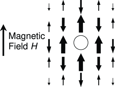
Figure 1: From Julien et al. (Ref. julien, ). Polarization of the Cu spins around the central Zn impurity (the circle) in the presence of an external field $H$, as measured julien by NMR on ${\rm YBa}_{2}{\rm Cu}_{3}{\rm O}_{6.7}$. The size of each arrow represents the value of the moment. Note that there is no spin directly on the Zn site, but it is expected that a net moment of $S=1/2$ centered at it at $T=0$.

It is worth emphasizing that $\mathcal{S}_{\text{imp}}$ is to be viewed as a long-wavelength theory for the impurity at site $r$, and requires some interpretation when applied to lattice models. In particular when a non-magnetic Zn or Li impurity replaces a spin-1/2 Cu ion, there is clearly no spin degree of freedom directly at the impurity site. Instead the spin polarization is distributed in a staggered arrangement on the neighboring Cu ions, so that the total moment is expected to be $S_{r}=1/2$ at $T=0$; this has been studied in elegant experiments alloul2 ; alloul2a ; julien , and we reproduce the results of one of these observations in Fig. 1. The unit vector $n_{r\alpha}$ then measures the instantaneous orientation of the collective spin polarization which is centered on a non-magnetic Zn site, and the Berry phase in (13) is the net uncompensated contribution obtained by summing over the Berry phases of all the spins on the neighboring Cu ions. The spatial correlations of the spins on the Cu ions are encoded, in our theory, in those of the $\phi_{\alpha}$ field.

Some crucial properties of the partition function $Z$ in (13) follow from simple power-counting arguments. We will perform these here at tree level, and higher loop corrections do not lead to corrections which modify the main conclusions. We focus here on the properties of a single impurity: the consequences of interactions between the impurities will be discussed later. We examine the behavior of $\mathcal{S}_{\text{b}}+\mathcal{S}_{\text{imp}}$ under a rescaling transformation $x\rightarrow x/b$ and $\tau\rightarrow\tau/b$ centered at the impurity (the dynamic critical exponent, $z$, is unity). The scaling dimensions of $\phi_{\alpha}$ and $n_{\alpha}$ are fixed by demanding invariance of the time derivative terms: this leads to

$$\text{dim}[\phi_{\alpha}]=(d-1)/2\quad;\quad\text{dim}[n_{\alpha}]=0.$$ (15)

These can be used to determine the dimension of $\gamma_{0r}$:

$$\text{dim}[\gamma_{0r}]=(3-d)/2.$$ (16)

So $\gamma_{0r}$ is a relevant perturbation about the decoupled fixed point in $d=2$. Following results of earlier work on related models SY2 ; si ; Sengupta , we find that in an expansion in

$$\epsilon=3-d,$$ (17)

$\gamma_{0r}$ reaches one of two fixed point values $\pm\gamma^{\ast}$ under the renormalization group (RG) flow (the value of $\gamma^{\ast}$ depends upon $S_{r}$, but we will not denote this explicitly). So the low energy properties of $Z$ are actually independent of the particular bare couplings $\gamma_{0r}$, and are controlled instead by $\gamma^{\ast}$. The memory of the initial values of $\gamma_{0r}$ is retained in the sign of the fixed point value: at the fixed point we have $\gamma_{0r}=\sigma_{r}\gamma^{\ast}$ where $\sigma_{r}=\pm 1$, and the sign of $\sigma_{r}$ is the same as that of the initial sign of $\gamma_{0r}$, i.e., $\gamma_{0r}$ does not change sign under the RG flow. The initial sign of $\gamma_{0r}$ is determined by sublattice location of the impurity in the host lattice antiferromagnet, and so both signs are equally probable.

Similar arguments can be used to show that there are no other relevant couplings between the impurity and the host antiferromagnet, consistent with the required symmetries. The simplest possible new coupling is

$$\sum_{r}\int d\tau\zeta_{r}\phi_{\alpha}^{2}(x=r,\tau),$$ (18)

which represents variation in the strength of the exchange constants in the vicinity of the impurity. Power counting shows that

$$\text{dim}[\zeta_{r}]=2-d.$$ (19)

So the $\zeta_{r}$ are strongly irrelevant for small $\epsilon$ (this is all that is needed, as the tree level arguments are valid only for small $\epsilon$). We can also consider the coupling of the impurity spin to the local uniform (ferromagnetic) magnetization density $L_{\alpha}$. For the action $\mathcal{S}_{\text{b}}$, the latter is given by book

$$L_{\alpha}=i\epsilon_{\alpha\beta\gamma}\phi_{\beta}\partial_{\tau}\phi_{\gamma};$$ (20)

and the coupling to the impurity spin takes the form

$$\sum_{r}\int d\tau\widetilde{\zeta}_{r}S_{r}L_{\alpha}(x=r,\tau)n_{r\alpha}(\tau).$$ (21)

Because $L_{\alpha}$ is the density of a conserved charge

$$\text{dim}[L_{\alpha}]=d,$$ (22)

and so

$$\text{dim}[\widetilde{\zeta}_{r}]=1-d,$$ (23)

and $\widetilde{\zeta}_{r}$ is also irrelevant. Similar arguments apply to all other possible couplings between the host and the impurities consistent with global symmetries.

(It is worth mentioning, parenthetically, that if we relax the constraint of global SU(2) symmetry, and allow for spin anisotropy, then relevant couplings are possible at the impurity site. The most important of these are a local field $\sum_{r}\int d\tau w_{r}n_{rz}(\tau)$, or a single-ion anisotropy $\sum_{r}\int d\tau\tilde{w}_{r}n_{rz}^{2}(\tau)$: the $w_{r}$, $\tilde{w}_{r}$ are easily seen to be relevant with scaling dimension 1. Now there is one relevant coupling in the bulk ($s$), and one or more on the impurity ($w_{r}$, $\tilde{w}_{r}$), and even the single-impurity problem has the topology of a multicritical phase diagram: separate phase transitions are possible at the impurity, the bulk, or both, and the full technology of boundary critical phenomena cardybook has to be used. For $S_{r}=1/2$ the single-ion anisotropy is inoperative, and if there is also no local field, we have to consider exchange anisotropies in the $\gamma_{0r}$, and these can also be relevantSengupta .)

We have now assembled all the ingredients necessary to establish our earlier assertion that no additional parameters are needed to describe the dynamics of the antiferromagnet in the presence of impurities. For the case of a single impurity (or a non-extensive density of impurities) our arguments show that there is only one relevant parameters at the quantum critical point—the ‘mass’ $s$; its scale is set by the spin gap, $\Delta$, for $s>s_{c}$ and by the spin stiffness, $\rho_{s}$, for $s<s_{c}$. All other couplings, whether they are bulk (like $g_{0}$) or associated with the impurities (like $\gamma_{0r}$) either flow to a fixed point value or are strongly irrelevant. We do need a parameter to set the relative scales of space and time, and this is the velocity $c$. Our arguments also allow us to obtain important information for the case where the density of impurities, $n_{\text{imp}}$, is finite. Now $n_{\text{imp}}$ itself is a relevant perturbation of the critical point; however, we can use the fact that there is no new energy scale which characterizes the coupling of a single impurity to the bulk antiferromagnet to conclude that the value of $n_{\text{imp}}$ alone is a complete measure of the strength of this perturbation.

Let us restate the above important conclusion a little more explicitly. Assume we are doping the spin gap paramagnet with $s>s_{c}$ and a spin gap, $\Delta$ (very similar arguments apply also for $s<s_{c}$ with $\rho_{s}$ replacing $\Delta$). For the case of a single impurity, the dynamics of the host antiferromagnet in the vicinity of the impurity is determined entirely by $\Delta$ and $c$ with no free parameters. A finite density of impurities, $n_{\text{imp}}$, is a relevant perturbation, but its impact is determined entirely by the single energy scale, $\Gamma$, that can be constructed out of the above parameters, and that is also linear in $n_{\text{imp}}$:

$$\Gamma\equiv\frac{n_{\text{imp}}(\hbar c)^{d}}{\Delta^{d-1}}.$$ (24)

In particular, all dynamic and thermodynamic properties of the host antiferromagnet are modified only by a universal dependence on the ratio $\Gamma/\Delta$; all corrections to these (including those dependent on the magnitude of the bare coupling between the impurity and host antiferromagnet) are suppressed by factors of $\Delta/J$, and only the latter are non-universal. The leading universal modification depends also on the statistics of the values of $S_{r}$ and $\sigma_{r}$: in most physical applications we simply have $S_{r}=S$ independent of $r$, while the $\sigma_{r}$ are independently distributed and take the values $\pm 1$ with equal probability.

The above universal dependence on $\Gamma/\Delta$ does not preclude the possibility that there could be a phase transition in the ground state as a function of $\Gamma/\Delta$: a magnetically ordered state could appear for infinitesimal doping, i.e., at $\Gamma/\Delta=0^{+}$, or at some finite critical value of $\Gamma/\Delta$— these two possible phase diagrams are shown in Fig 2.

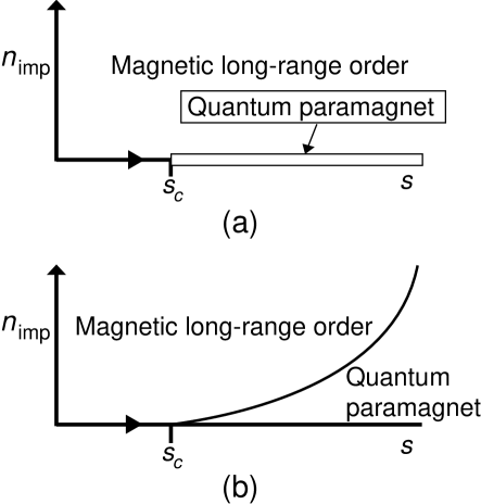
Figure 2: Two possible phase diagrams of the quantum field theory $\mathcal{S}_{\text{b}}+\mathcal{S}_{\text{imp}}$ for a dilute concentration of impurities $n_{\text{imp}}$. For $s>s_{c}$, all low energy properties depend only upon the dimensionless ratio $\Gamma/\Delta$, where $\Delta$ is the spin gap of the undoped host antiferromagnet, and $\Gamma$ is defined in (24). In (a) there is a phase transition to an ordered state at $\Gamma/\Delta=0^{+}$, and a quantum paramagnet is present only for $n_{\text{imp}}=0$ and $s>s_{c}$; in (b) the transition to the ordered state occurs at some finite universal value of $\Gamma/\Delta$, and so by (9,24) the phase boundary obeys $n_{\text{imp}}\sim(s-s_{c})^{\nu d}$. For $s<s_{c}$ the properties are universal functions of the analogous dimensionless ratio $n_{\text{imp}}(\hbar c/\rho_{s})^{2}$ (where $\rho_{s}$ is the stiffness of the host antiferromagnet); we have not shown a third possible phase diagram in which the phase boundary is present for $s<s_{c}$ with $n_{\text{imp}}\sim(s_{c}-s)^{\nu d}$. Right at $s=s_{c}$, the spacetime correlators are universal function of the dimensionless combinations $xn_{\text{imp}}^{1/d}$ and $c\tau n_{\text{imp}}^{1/d}$ with no arbitrary scale factors. For any lattice antiferromagnet, the long-range order will disappear at sufficiently large $n_{\text{imp}}$ when the concentration of impurities is near the percolation threshold—this phase boundary has not been shown in the figure, as it is not a property of the continuum theory $\mathcal{S}_{\text{b}}+\mathcal{S}_{\text{imp}}$. This latter transition was considered by Chen and Castro Neto antonio , along with the behavior as a function of $n_{\text{imp}}$ for $s<s_{c}$; however, they did not include the Berry phases, and these are expected to be important in the critical region SY .

Determination of the phase diagram requires solution of the problem of interacting quantum impurities; in the paramagnetic phase ($s>s_{c}$), an effective action for interactions can be obtained by integrating out the $\phi_{\alpha}$ fields from $\mathcal{S}_{\text{b}}+\mathcal{S}_{\text{imp}}$. Apart from the same Berry phase terms in $\mathcal{S}_{\text{imp}}$, the resulting action contains the term

$$-\sum_{r\neq r^{\prime}}\int\!\!d\tau\!\!\int\!\!d\tau^{\prime}S_{r}S_{r^{\prime}}\sigma_{r}\sigma_{r^{\prime}}D(r-r^{\prime},\tau-\tau^{\prime})n_{r\alpha}(\tau)n_{r^{\prime}\alpha}(\tau^{\prime}),$$ (25)

where the universal interaction $D$ is proportional to the $\phi_{\alpha}$ propagator and depends only on the fixed point value $\gamma^{\ast}$ (which is an implicit function of $S_{r}$)—$D$ decays exponentially for large $|r-r^{\prime}|$ or $|\tau-\tau^{\prime}|$; there are additional multi-spin interactions between the impurities which have not been displayed. A notable propertysigrist1 ; imada of (25) is that the signs of the interactions have the disorder of the “Mattis model”mattis , i.e., there is no frustration, and the product of interactions around any closed loop has a ferromagnetic sign. However, unlike the classical spin glass, the fluctuating signs of the exchange interaction cannot be gauged away in this quantum Mattis model, as the transformation $n_{\alpha}\rightarrow-n_{\alpha}$ is not a symmetry of the Berry phase term (equivalently, it does not preserve the spin commutation relations). Nevertheless, the absence of frustration in such a model has been used by Nagaosa et al. sigrist1 and Imada and Iino imada to argue in favor of the phase diagram in Fig 2a.

We reiterate that, irrespective of the correct phase diagram, all low energy properties depend only the value of the dimensionless ratio $\Gamma/\Delta$, which is a measure of the strength of the relevant perturbation of a finite concentration of impurities. It is remarkable that such a measure is independent of the magnitude of the exchange coupling between the impurities and the antiferromagnet. We also note that some of the earlier scaling arguments of Imada and Iino imada are contained in such an assertion—it implies their identification of the crossover exponent of the impurity density as $\nu d$.

I.2.1 Application to d-wave superconductors

While it is reasonably transparent that the action $\mathcal{S}_{\text{b}}+\mathcal{S}_{\text{imp}}$ applies to the Zn doping of insulating spin gap compounds like ${\rm SrCu}_{2}{\rm O}_{3}$, the applicability to Zn doping of a good d-wave superconductor like ${\rm Y}{\rm Ba}_{2}{\rm Cu}_{3}{\rm O}_{7}$ has not yet been established. Actually the similarity of Zn doping in a cuprate superconductor to that of spin gap compounds was already noted by the experimentalists in Ref keimer, —here we will sharpen their proposal.

There is a great deal of convincing experimental evidence that each Zn impurity has an antiferromagnetic polarization of Cu ions in its vicinity, and the net moment of this polarization is expected to be $S_{r}=1/2$ at $T=0$; at moderate temperature this moment precesses freely giving rise to a Curie susceptibility, while there is evidence for spin freezing at very low temperatures, presumably from inter-impurity interactions (see Fig. 1, Refs. alloul2, ; tomo, ; alloul2a, ; julien, and references therein). The Berry phase term in $\mathcal{S}_{\text{imp}}$ then encodes the dynamics of the collective precession of the spins on the Cu ions near the Zn impurity at site $r$ (recall that there is no spin on the Zn ion itself).

The impurity spin will couple to spin excitations in the host superconductor. The most important of these is the spin-1 collective mode which gives rise to the ‘resonance peak’ rossat1 ; mook ; tony3 ; bourges ; he of the cuprate superconductors. In our approach CSY this collective mode is represented by the oscillation of the field $\phi_{\alpha}$ about $\phi_{\alpha}=0$ controlled by the action $\mathcal{S}_{\text{b}}$. So our picture of the resonance peak is similar in spirit to computations levin ; morr ; brinck which identify it with a $S=1$ bound state in the particle-hole channel in RPA-like theories of the dynamic spin response of a d-wave superconductor. However, such theories use a weak-coupling BCS picture of the electron spin correlations and also neglect the non-linear self-interactions of the collective mode. In contrast, in our approach the underlying spin correlations are characterized by $\mathcal{S}_{\text{b}}$, which assumes that the superconductor is close to an insulating state with magnetic long-range order (and possibly also charge order): this has the advantage of allowing a systematic treatment of the strongly relevant quartic non-linearity in the $\phi_{\alpha}$ field, and these non-linear effects are crucial to the universal nature of our results. We also mention the approach of Zhang zhang which assumes that 3-component $\phi_{\alpha}$ is part of 5-component “superspin”—unlike Zhang, our theory does not appeal to any higher (approximate) symmetry group in the superspin action, beyond that expected from spin rotation invariance.

Spin is also carried by the fermionic, spin-1/2 Bogoliubov quasiparticles in a d-wave superconductor, and these will couple to the impurity spin. These quasiparticles have vanishing energy at four points in the Brillouin zone - $(\pm K,\pm K)$. As is well known, a gradient expansion the of low energy fermionic excitations in the vicinity of these points yields an action that can be expressed in terms of 4 species of anisotropic Dirac fermions. We do not wish to enter into the specific details of this action here, as only some gross features will be adequate for our basic argument. Let us represent these fermions schematically by the Nambu spinors $\Psi$; then the action has the form

$$\mathcal{S}_{\Psi}=\int d^{2}xd\tau\left[\Psi^{\dagger}\partial_{\tau}\Psi+\Psi^{\dagger}\nabla_{x}\Psi\right].$$ (26)

We have omitted all coupling constants and matrices in the Nambu and spin spaces, as we do not need to know their structure here. The important point is that this action implies the dimension

$$\text{dim}[\Psi]=1$$ (27)

under scaling transformations.

Now let us couple $\Psi$ to the degrees of freedom in ${\cal S}_{\text{b}}+\mathcal{S}_{\text{imp}}$.

There will be a bulk cubic coupling of the form $\phi_{\alpha}\Psi\Psi$ or $\phi_{\alpha}\Psi^{\dagger}\Psi$ only if it is permitted by the momentum conservation in the host antiferromagnet. As the $\phi_{\alpha}$ represent spin fluctuations at the wavevector ${\bf Q}$, such a cubic coupling is permitted only if ${\bf Q}$ equals the sum or difference of two of $(\pm K,\pm K)$ (i.e. if ${\bf Q}=(2K,2K)$ or not). For simplicity, in the body of the paper, we will assume in this is not the case, i.e. we assume ${\bf Q}\neq(2K,2K)$. Indeed, in ${\rm Y}{\rm Ba}_{2}{\rm Cu}_{3}{\rm O}_{7}$, ${\bf Q}=(\pi,\pi)$ and it appears that $K\neq\pi/2$, and so a cubic term is forbidden. However, $K$ is not too far from $\pi/2$, and so the effect of a cubic term may be manifest at higher energies. In Appendix A we consider the limiting case ${\bf Q}=(2K,2K)$, which permits a cubic term in the host d-wave superconductor at the lowest energies. A renormalization group analysis of such a host theory was presented recently by Balents et al.balents , and Appendix A combines their results with the quantum impurity theory of the present paper: we find that the scaling structure is essentially identical to that in the body of the paper, and there are only simple quantitative modifications to the fixed-point values of the couplings.

For now, we assume that momentum conservation prohibits a bulk coupling between the bosonic ($\phi_{\alpha}$) and fermionic ($\Psi$) carriers of spin caveat . However these degrees of freedom can still interact via their separate couplings to the impurity spins. The coupling of the superconducting quasiparticles to the impurities at sites $\{r\}$ is of the form

$$\mathcal{S}_{\Psi\text{imp}}=\sum_{r}\int d\tau\big{[}J_{r}S_{r}n_{r\alpha}(\tau)\Psi^{\dagger}(x=r,\tau)\Psi(x=r,\tau)$$

$$\quad+J_{r}^{\prime}S_{r}n_{r\alpha}(\tau)\Psi(x=r,\tau)\Psi(x=r,\tau)+\text{H.c.}$$

$$\quad+V_{r}\Psi^{\dagger}(x=r,\tau)\Psi(x=r,\tau)$$

$$\quad+V_{r}^{\prime}\Psi(x=r,\tau)\Psi(x=r,\tau)+\text{H.c.}\big{]}.$$ (28)

Again, we have omitted matrices in spin and Nambu space; the $J_{r}$, $J_{r}^{\prime}$ are exchange couplings between the quasiparticles and the Cu spins in the vicinity of the Zn impurity, and the $V_{r}$, $V_{r}^{\prime}$ represent potential scattering terms from the non-magnetic Zn ion itself. Models closely related to $\mathcal{S}_{\Psi}+\mathcal{S}_{\Psi\text{imp}}$ have been the subject of a large number of studies in the past few years lee ; sasha1 ; sasha2 ; kallin ; fradkin ; nl ; sigrist2 ; ogata ; fulde ; pepin and a number of interesting results have been obtained. However, all of these earlier works have not included a coupling between the impurity spin and a collective, spin-1, bosonic mode like $\phi_{\alpha}$. One of the central assertions of this paper is that (provided the spin gap, $\Delta$, is not too large) such a coupling (as in $\mathcal{S}_{\text{imp}}$) is of paramount importance for the low energy spin dynamics, while the coupling to the superconducting quasiparticles (as in $\mathcal{S}_{\Psi\text{imp}}$) has weaker effects.

(However, when one is explicitly interested in quasiparticle properties, as in tunneling experiments, it is certainly necessary to include $\mathcal{S}_{\Psi}+\mathcal{S}_{\Psi\text{imp}}$; in STM experiments with atomic resolution seamus , the quasiparticle tunneling can be observed directly at the Zn site, and there the potential scattering terms $V_{r}$,$V_{r}^{\prime}$ will be especially important as there is no magnetic moment (see Fig 1). As we noted below (14), we are considering a long-wavelength theory of the spin dynamics, and careful interpretation is required for lattice scale effects.)

The argument behind our assertion is quite simple. Using (27) we see that

$$\text{dim}[J_{r},J_{r}^{\prime},V_{r},V_{r}^{\prime}]=-1.$$ (29)

Therefore, while the couplings, $\gamma_{0r}$, between the impurities and the $\phi_{\alpha}$ had a positive scaling dimension in (16), those between the fermionic quasiparticles and the impurities have a negative dimension and are strongly irrelevant. We are therefore justified in neglecting the fermionic quasiparticles in our discussion of the impurity spin dynamics.

The above conclusion is also supported by studies withoff ; CJ ; ingersent ; bulla ; isi of models related to $\mathcal{S}_{\Psi}+\mathcal{S}_{\Psi\text{imp}}$ in the context of “Kondo problems with a pseudogap in the fermionic density of the states”: for the case where the fermionic density of states vanishes linearly at the Fermi level (as is the case for $\mathcal{S}_{\Psi}$), there is no Kondo screening for small and moderate $J_{r}$, $J_{r}^{\prime}$ values, and the impurity spin is essentially static. Of course, the present renormalization group argument cannot rule out the possibility of new physics, associated with the fermionic Kondo effect, appearing at very large $J_{r}$, $J_{r}^{\prime}$: we shall assume that the bare couplings are in a regime such that this has not happened, and the scaling dimensions in (29) continue to apply.

I.3 Results

We will state our main results for the case of a single impurity in Section I.3.1, and those for a finite density in Section I.3.2.

I.3.1 Single Impurity

We first consider a single impurity at the origin of co-ordinates $x=0$ with

$$S_{r=0}\equiv S\quad;\quad n_{r=0,\alpha}(\tau)\equiv n_{\alpha}(\tau).$$ (30)

An important measurable response function is the impurity susceptibility defined in (11). Its properties follow simply from a naive application of the scaling ideas we have presented above, and are summarized in Fig 3.

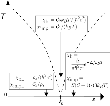
Figure 3: Summary of the results for the bulk and impurity susceptibilities of $\mathcal{S}_{\text{b}}+\mathcal{S}_{\text{imp}}$ in $d=2$ with a single impurity at the origin of co-ordinates with $S_{r}=S$. The dashed lines represent crossover boundaries. The crossover for $s>s_{c}$ occurs when $\Delta\sim k_{B}T$, and is between the high-temperature ‘quantum critical’ regime and the low-temperature quantum paramagnet described by a dilute gas of spin-1 $\phi_{\alpha}$ quanta. Similarly, the crossover for $s<s_{c}$ occurs when $\rho_{s}\sim k_{B}T$, and the low-temperature regime is a locally ordered Néel state whose long range order is disrupted by long-wavelength, classical, spin-wave fluctuations. The constants ${\cal C}_{1-3}$ are universal numbers, insensitive to microscopic details. The constant ${\cal C}_{2}$ was introduced in Ref CS, , and is determined solely by the bulk theory $\mathcal{S}_{\text{b}}$; quantum Monte Carlo results were obtained in Ref troyer, . The constants ${\cal C}_{1}$ and ${\cal C}_{3}$ are determined by $\mathcal{S}_{\text{b}}+\mathcal{S}_{\text{imp}}$, and depend only on the integer/half-odd-integer valued $S$. The constant ${\cal C}_{1}$ defines the effective spin at the quantum-critical point by ${\cal C}_{1}=S_{\rm eff}(S_{\rm eff}+1)/3$, and $S_{\rm eff}$ is neither an integer nor a half-odd-integer. On the ordered side, $s<s_{c}$, in the absence of even an infinitesimal spin anisotropy, the measured spin susceptibility will take the rotationally averaged value Science $\chi_{\rm imp}=S^{2}/(3k_{B}T)+(2/3)\chi_{{\rm imp}\perp}$; we have no reason to expect non-monotonic behavior of the susceptibility as a function of $s$, and so this result suggests the bounds $S^{2}/3<\mathcal{C}_{1}<S(S+1)/3$ in $d=2$.

Knowledgeable readers may be surprised by such an assertion. In the intensively studied multichannel Kondo quantum impurity problem noz naive scaling actually fails: even though the low energy physics is controlled by a finite coupling quantum critical point, a ‘compensation’ effect barzykin causes most thermodynamic response functions to vanish in the naive scaling limit, and the leading low temperature behavior is exposed only upon considering corrections to scaling AL ; OPAG . Fortunately, our problem is simpler—the bosonic $\phi_{\alpha}$ excitations which ‘screen’ the impurity are themselves controlled by a non-trivial interacting quantum field theory ${\cal S}_{\text{b}}$, and it is not possible to ‘gauge away’ the effect of an external magnetic field on them.

Armed with this reassuring knowledge, we need only know that $\chi_{\text{imp}}$ has the dimensions of inverse energy to deduce its critical properties. For $s>s_{c}$ we of course have the Curie response in (12), which is, not coincidentally, also consistent with the scaling requirements. At the critical coupling $s=s_{c}$, we continue to have a Curie-like response (because now $k_{B}T$ is the only available energy scale) but can no-longer require that the effective moment be quantized:

$$\chi_{\text{imp}}=\frac{{\cal C}_{1}}{k_{B}T}\quad;\quad T>|s-s_{c}|^{\nu}.$$ (31)

The universal number ${\cal C}_{1}$ is almost certainly irrational, and we will estimate its value in Sections II.2 and III.4; our most reliable estimate for $S=1/2$ and $d=2$ is in (163), with $\mathcal{C}_{\text{free}}=1/4$. Turning finally to $s<s_{c}$, the $T=0$ response is now anisotropic because of the Néel order in the ground state. We consider here only the response transverse to the Néel order, $\chi_{\perp}$, at $T=0$; further details are in Section II.3.2. The same scaling arguments now imply

$$\chi_{\text{imp}\perp}=\frac{{\cal C}_{3}}{\rho_{s}}\quad;\quad T=0,~{}d=2,~{}s<s_{c}.$$ (32)

Again ${\cal C}_{3}$ is an irrational universal number whose value will be estimated later.

Having described the response to a uniform, global magnetic field, let us consider the responses to local probes in the vicinity of the impurity. Such results will apply to NMR and tunneling experiments. In considering such response function it is useful to use the language of boundary conformal field theory cardybook : we are considering here a bulk $(d+1)$-dimensional conformal field theory, $\mathcal{S}_{\text{b}}$ at $s=s_{c}$, which contains a one-dimensional ‘boundary’ degree of freedom at $x=0$. Correlation functions near the boundary will be controlled by boundary scaling dimensions which are distinct from the scaling dimensions of the bulk theory we have considered so far. The most important of these controls the long-time decay of the impurity spin:

$$\langle n_{\alpha}(\tau)n_{\alpha}(0)\rangle\sim\frac{1}{\tau^{\eta^{\prime}}}\quad;\quad s=s_{c},~{}T=0,~{}\tau\rightarrow\infty.$$ (33)

(Here, and in the remainder of the paper we are indulging in a slight abuse of terminology by identifying these as the correlations of the “impurity spin”; as in Fig 1 it is often the case that there is no spin on the impurity site—in such cases we are referring to spin correlations at sites very close to the impurity.) The quantity $\eta^{\prime}$ is an anomalous boundary exponent: we will compute its value in the expansion in $\epsilon$ in Section II.1. Clearly, (33) implies the scaling dimension

$$\text{dim}[n_{\alpha}]=\eta^{\prime}/2,$$ (34)

which corrects the tree-level result in (15). (This is a good point to mention that loop corrections also modify the scaling dimension of the bulk field $\phi_{\alpha}$ in (15) to

$$\text{dim}[\phi_{\alpha}]=(d-1+\eta)/2,$$ (35)

where $\eta$ (like $\nu$) is a known exponent which is a property of $\mathcal{S}_{\text{b}}$ alone book .)

For $s\neq s_{c}$, there is a finite remnant moment in the boundary spin correlations. For $s<s_{c}$, this is simply a consequence of the bulk Néel order also breaking the spin rotation symmetry on the boundary too. However, for $s>s_{c}$, this is a somewhat more non-trivial quantum effect: the presence of the spin gap in the bulk, means that the boundary excitations, associated with the Berry phase term in $\mathcal{S}_{\text{imp}}$ are confined to the impurity and maintain a permanent static moment. So we may generalize (33) to

$$\lim_{\tau\rightarrow\infty}\langle n_{\alpha}(\tau)n_{\alpha}(0)\rangle=m_{\text{imp}}^{2}\quad;\quad T=0.$$ (36)

The impurity moment, $m_{\text{imp}}$, (the remarks below (33) on abuse of terminology apply to the “impurity moment” too) behaves like

$$m_{\text{imp}}\sim|s-s_{c}|^{\eta^{\prime}\nu/2},$$ (37)

a consequence of the scaling dimension (34).

We have computed a large number of correlation functions describing the spatial and temporal evolution of the spin correlations in the vicinity of the impurity. We will leave a detailed discussion of these to the body of the paper, but note here some simple arguments which allow deduction of important qualitative features. The experimental probes mentioned earlier can follow the spatial evolution of the correlators of the bulk antiferromagnetic order parameter field $\phi_{\alpha}$, and also that of the uniform (ferromagnetic) magnetization density $L_{\alpha}$. As the spatial arguments of $\phi_{\alpha}(x,\tau)$ and $L_{\alpha}(x,\tau)$ approach the impurity, their critical correlations must mutate onto those of the boundary degrees of freedom. This transformation is encoded in the statements of the operator product expansion

$$\lim_{x\rightarrow 0}\phi_{\alpha}(x,\tau) \sim \frac{n_{\alpha}(\tau)}{|x|^{(d-1+\eta-\eta^{\prime})/2}}$$

$$\lim_{x\rightarrow 0}L_{\alpha}(x,\tau) \sim \frac{n_{\alpha}(\tau)}{|x|^{d-\eta^{\prime}/2}},$$ (38)

where the powers of $x$ follow immediately from the scaling dimensions (34,35,22). The results (33) and (38) can be combined with scaling arguments to determine the important qualitative features of the spatial, temporal, and temperature dependencies of most observables in the vicinity of the impurity: details appear in Sections II.2 and II.3.

I.3.2 Finite density of impurities

The problem of a finite density of impurities is one of considerable complexity, and we will only address a particular aspect for which we have new, significant, and experimentally testable predictions. We will not settle the issue of whether Fig 2a or b, or some other possibility, is the correct phase diagram.

We will be interested in dynamical properties of the region, $s>s_{c}$, as characterized by the susceptibility at the antiferromagnetic wavevector

$$\chi_{{\bf Q}}(\omega_{n})=\int\!\!\frac{d^{d}xd^{d}x^{\prime}}{V}\int_{0}^{\beta}\!\!\!d\tau\langle\phi_{\alpha}(x,\tau)\phi_{\alpha}(x^{\prime},0)\rangle e^{i\omega_{n}\tau},$$ (39)

where $V$ is the volume of the system, and $\omega_{n}$ is a Matsubara imaginary frequency. In the absence of impurities in an insulating antiferromagnet, this susceptibility has a pole at the spin gap energy CSY (at $T=0$):

$$\chi_{{\bf Q}}(\omega)=\frac{\mathcal{A}}{\Delta^{2}-(\hbar\omega+i0^{+})^{2}},$$ (40)

where $\omega$ is now a real frequency, $0^{+}$ represents a positive infinitesimal, and $\mathcal{A}$ is a residue determining the spectral weight of the spin-1 collective mode. The form in (40) is valid only in the vicinity of the pole, and quite complicated structures appear well away from the pole frequency. Such a pole will also be present in a d-wave superconductor if momentum conservation prohibits decay of $\phi_{\alpha}$ into low-energy fermionic $\Psi$ quasiparitcles. The case for which such a decay is allowed is considered in Appendix A: we show there that (40) is replaced by the more general scaling form

$$\chi_{{\bf Q}}(\omega)=\frac{\mathcal{A}}{\Delta^{2}}\Phi_{0}\left(\frac{\hbar\omega}{\Delta}\right),$$ (41)

where $\Phi_{0}$ is a universal scaling function. The form (41) predicts that in such d-wave superconductors the pole in (40) will be universally broadened on an energy scale $\Delta$. Such a pole (or broadened pole) has immediate experimental consequences: it leads to a ‘resonance peak’ in the neutron scattering cross-section, as is seen in ${\rm Y}{\rm Ba}_{2}{\rm Cu}_{3}{\rm O}_{7}$ rossat1 ; mook ; tony3 ; bourges ; he . At current experimental resolution, no intrinsic broadening has been observed at low temperatures, and so it is reasonable in a first theory to work with the sharp pole in (40), as we do in the body of this paper.

Our primary interest will be in the fate of the pole (or of (41)) in the presence of a finite density of impurities, $n_{\text{imp}}$. This is a property at the energy scale of order $\Delta$, and useful results can be obtained without resolving the very low energy properties which distinguish the phase diagrams of Fig 2. At small $n_{\text{imp}}$, the typical interaction $D$ in (25) is exponentially small in $(\Delta/\Gamma)^{1/2}$, and we will neglect such effects. Instead, at the energy scales we are interested in, we use mean-field approach to account for a finite $n_{\text{imp}}$, but include the full dynamics of the interaction between the $\phi_{\alpha}$ and a single impurity: the finite $n_{\text{imp}}$ will only modify the density of states of the $\phi_{\alpha}$ excitations, and this will be determined self-consistently.

Let us first review the exact scaling arguments. The expression (39) defines a bulk observable which cannot acquire any of the anomalous boundary dimensions. Consequently its deformation due to the impurities is fully determined only by the energy scale $\Gamma$ defined in (24), and we have the scaling prediction that (40) is modified to

$$\chi_{{\bf Q}}(\omega)=\frac{\mathcal{A}}{\Delta^{2}}\Phi\left(\frac{\hbar\omega}{\Delta},\frac{\Gamma}{\Delta}\right),$$ (42)

where $\Phi$ is a fully universal function of its arguments (we have restricted attention to $T=0$ here—for $T>0$ there is universal dependence on an additional argument, $T/\Delta$). For the case where there is no bulk coupling to fermionic quasiparticles at the lowest energies, we have $\Phi(\overline{\omega},0)=1/(1-(\overline{\omega}+i0^{+})^{2})$, and so (42) reduces to (40) for zero impurity density, $\Gamma=0$; with a bulk coupling of $\phi_{\alpha}$ to fermionic quasiparticles, as in Appendix A, (42) reduces to (41) at $\Gamma=0$. The scaling form (42) applies to the dynamic susceptibility for both possibilities of the phase diagram in Fig 2; if Fig 2b is the correct phase diagram, then the scaling function $\Phi$ will have a singularity at the critical value of $\Gamma/\Delta$.

Notice that the impurities induce broadening at an energy scale $\Gamma\sim 1/\Delta$. On the other hand, intrinsic broadening is suppressed by momentum conservation; in the special case that ${\bf Q}=(2K,2K)$, intrinsic broadening exists at the lowest energies, and then it is at most of order $\Delta$. So for small $\Delta$, the impurity broadening dominates in both cases. In experimental comparisons it may be useful to use fits with a linewidth written as a sum of intrinsic and extrinsic contributions. Further discussion of these issues is in Appendix A.

We will obtain results for the form of $\Phi$ for non-zero $\Gamma/\Delta$ in Section IV in a self-consistent non-crossing approximation, for the case where the coupling to fermionic quasiparticles is irrelevant. As we mentioned earlier, one of our important results will be that the $\Gamma>0$ lineshape has an asymmetric shape, with a tail at high frequencies. This is a significant prediction of our theory, which should be testable in future experiments. The experiment of Ref. keimer, has $S_{r}=1/2$, $\Gamma=5$ meV, $\Gamma/\Delta=0.125$ and we display our predicted lineshape for this value of $\Gamma/\Delta$ in Fig 4 (results for other values of $\Gamma/\Delta$ appear in Section IV). The half-width of the line is approximately $\Gamma$, and this is in excellent accord with the measured linewidth of 4.25 meV. The sharp lower threshold in the spectral weight is an artifact of the non-crossing approximation: consideration of Griffths effects (which, in principle, are contained in the exact scaling function in (42)), or the contribution of the “irrelevant” fermionic excitations (which are not part of the scaling limit (42), will always lead to a small rounding of the lower edge.

Figure 4: The universal lineshape $\text{Im}\Phi$ as a function of $\hbar\omega/\Delta$ for $d=2$, $S_{r}=1/2$, and $\Gamma/\Delta=0.125$, the values corresponding to the experiment of Ref. keimer, . This result has been obtained in a self-consistent ‘non-crossing approximation’ analysis of $\mathcal{S}_{\text{b}}+\mathcal{S}_{\text{imp}}$ described in Section IV.

I.4 Outline

We now sketch the contents of the remainder of the paper. Readers not interested in details of the derivation of the results may wish to skip ahead to Section V. Section II will obtain renormalization group results in an expansion in $\epsilon=3-d$ for the single impurity problem. Similar physical results will be obtained in Section III, but in a different large-$N$ or ‘non-crossing’ approximation (NCA). The advantage of the latter approach is that it can be readily extended to obtain a self-consistent theory of the magnon lineshape broadening; this shall be presented in Section IV. We review our main results and discuss some further experimental issues in Section V. The appendices contain extensions and further calculational details; in particular, Appendix A considers the case where momentum conservation allows a bulk coupling to the fermionic quasiparticles of a d-wave superconductor at the lowest energies, while Appendix B generalizes our results to antiferromagnets and d-wave superconductors with incommensurate spin correlations i.e. ${\bf Q}\neq(\pi,\pi)$.

II Expansion in $\epsilon=3-d$

The central ingredient behind the universal structure of all of our results is the analysis of the renormalization group equations presented in Section II.1. This is performed order-by-order in an expansion in $\epsilon=3-d$. The results will be used to obtain expressions for a number of physical observables in the subsequent subsections: we will consider the paramagnetic region, $s\geq s_{c}$, in Section II.2, and the magnetically ordered phase, $s<s_{c}$, in Section II.3.

All of the computations in this section will consider only the single impurity problem. We will therefore use the notation in (30) and also denote

$$\gamma_{0,r=0}\equiv\gamma_{0}.$$ (43)

Also in the remainder of this paper, we will use units of time, temperature, and length in which

$$\hbar=k_{B}=c=1.$$ (44)

II.1 Renormalization group equations

We will follow the orthodox field theoretic approach bgz in obtaining the renormalization group equations of $\mathcal{S}_{\text{b}}+\mathcal{S}_{\text{imp}}$: generate perturbative expansions for various observables correlators, multiply them with renormalization factors to cancel poles in $\epsilon$, and finally use the independence of the bare theory on the renormalization scale to obtain the scaling equations. This approach is rather abstract, but has the advantage of allowing explicit calculations to two-loop order and establishing important scaling relations to all orders. A more physically transparent ‘momentum shell’ formalism can be used to obtain equivalent results at one loop, but several key properties are not delineated at this order.

It is clearly advantageous to have a diagrammatic method which allows expansion of the correlators in powers of the couplings $g_{0}$ and $\gamma_{0}$. While the standard time-ordered perturbation theory can be used for $g_{0}$, the non-linear Berry phase term in $\mathcal{S}_{\text{imp}}$ (and the associated unit length constraint on $n_{\alpha}$) makes the expansion in $\gamma_{0}$ more intricate. Building on earlier work in the context of the Kondo problemhewson , we have developed a diagrammatic representation of the perturbative expansion in $\gamma_{0}$—this is described in Appendix C. The representation works to all orders in $\gamma_{0}$, but does not have the benefit of a Dyson theorem or the cancellation of disconnected diagrams; nevertheless, all terms at a given order in perturbation theory can be rapidly written down. For instance, the diagrams shown in Fig 5 lead to the following lowest order representation of the two-point correlator of $n_{\alpha}$ in the paramagnetic phase:

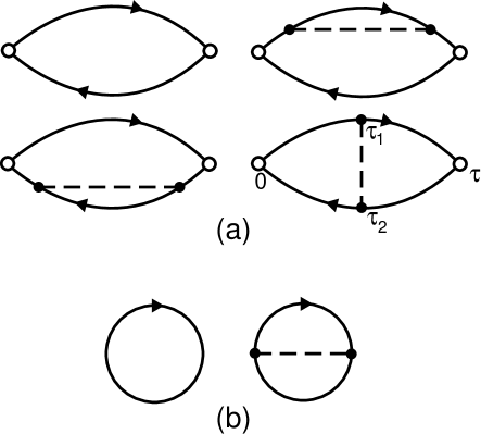
Figure 5: Representation of the correlation function in (45) in the diagrammatic approach of Appendix C. The open circles represent the external sources, the dashed lines are $\phi_{\alpha}$ propagators, and the filled circles contribute factors of $\gamma_{0}$. The impurity spin is represented by the single full line along which imaginary time runs periodically from 0 to $\beta$. The correlator (45) is the ratio of the diagrams in (a) to those in (b), with the latter representing the normalizing partition function $Z$.

$$S^{2}\langle n_{\alpha}(\tau)n_{\alpha}(0)\rangle=S(S+1)\bigg{[}1$$

$$\qquad\qquad-\gamma_{0}^{2}\int_{0}^{\tau}d\tau_{1}\int_{\tau}^{\beta}d\tau_{2}D(\tau_{1}-\tau_{2})+\cdots\bigg{]}$$ (45)

where $\tau>0$ and $D(\tau)$ is the two-point $\phi_{\alpha}$ propagator at $x=0$

$$D(\tau) = \langle\phi_{\alpha}(0,\tau)\phi_{\alpha}(0,0)\rangle_{0}$$ (46)

$$\equiv T\sum_{\omega_{n}}\int\frac{d^{d}k}{(2\pi)^{d}}\frac{e^{-i\omega_{n}\tau}}{\omega_{n}^{2}+k^{2}+m^{2}}.$$

Here the 0 subscript in the correlator indicates that it is evaluated to zeroth order in $g_{0}$. However, we have included Hartree-Fock renormalizations in the determination of the ‘mass’ $m$; these have been computed in earlier work in the $\epsilon$ expansion ss , and we quote some limiting cases:

$$m=\left\{\begin{array}[]{ll}\Delta&\quad;\quad s\geq s_{c},~{}T\ll\Delta\\ \left(10\epsilon/33\right)^{1/2}\pi T&\quad;\quad T\gg|s-s_{c}|^{\nu}\end{array}\right..$$ (47)

Recall that $\Delta$ was defined earlier as the exact $T=0$ spin gap of the host antiferromagnet. The crossover function between the two limiting results in (47) is also known for small $\epsilon$, but we refer the reader to the original paper ss for explicit details.

The $T=0$ limit of (45) must be taken with some care: the function $D(\tau)$ in (46) is periodic as a function of $\tau$ with period $\beta$, and so any significant contributions for small $|\tau|$ have periodic images in the region with small $|\beta-\tau|$. Indeed, at $T=0$, and at the critical coupling $s=s_{c}$ (where $m=\Delta=0$), (45) reduces to

$$S^{2}\langle n_{\alpha}(\tau)n_{\alpha}(0)\rangle=S(S+1)\bigg{[}1$$

$$-\gamma_{0}^{2}\int_{0}^{\tau}d\tau_{1}\bigg{(}\int_{\tau}^{\infty}d\tau_{2}+\int_{-\infty}^{0}d\tau_{2}\bigg{)}D_{0}(\tau_{1}-\tau_{2})\bigg{]},$$ (48)

where

$$D_{0}(\tau) = \int\frac{d^{d}k}{(2\pi)^{d}}\frac{d\omega}{2\pi}\frac{e^{-i\omega\tau}}{k^{2}+\omega^{2}}$$ (49)

$$\equiv \frac{\widetilde{S}_{d+1}}{\tau^{d-1}},$$

with

$$\widetilde{S}_{d}=\frac{\Gamma(d/2-1)}{4\pi^{d/2}}.$$ (50)

Simple power counting of the integrals in (48) shows that they lead to poles in $\epsilon$–this is as expected from the tree-level scaling dimension of $\gamma_{0}$ in (16). In the field theoretic RG these poles have to be cancelled by appropriate renormalization factors which we will describe shortly. Evaluating the integrals in (48), and also those in the two-loop corrections to (48) described in Appendix C, we obtain

$$S^{2}\langle n_{\alpha}(\tau)n_{\alpha}(0)\rangle=S(S+1)\bigg{[}1-\frac{2\gamma_{0}^{2}\widetilde{S}_{d+1}\tau^{\epsilon}}{\epsilon(1-\epsilon)}$$

$$\qquad+\big{(}\gamma_{0}^{2}\widetilde{S}_{d+1}\tau^{\epsilon}\big{)}^{2}\left(\frac{4}{\epsilon^{2}}+\frac{9}{\epsilon}+\ldots\right)\bigg{]}.$$ (51)

We have retained only poles in $\epsilon$ in the co-efficient of the $\gamma_{0}^{4}$ term, as that is all that shall be necessary for our subsequent analysis.

We now describe the structure of the renormalization constants that are needed to cancel the poles in (51) and in other observable correlation functions. First, the renormalization factors of the host antiferromagnet can only depend upon the bulk theory $\mathcal{S}_{\text{b}}$ as a single impurity cannot make a thermodynamically significant contributions. These are well known and described in numerous text books and review articles; we will use here the conventions of Brezin et al.bgz They define the renormalized field $\phi_{R\alpha}$ and the dimensionless coupling constant, $g$ by

$$\phi_{\alpha} = Z^{1/2}\phi_{R\alpha}$$

$$g_{0} = \frac{\mu^{\epsilon}Z_{4}}{Z^{2}S_{d+1}}g,$$ (52)

where $\mu$ is a renormalization momentum scale, $Z$ is the wave-function renormalization factor of the field $\phi_{\alpha}$, $Z_{4}$ is a coupling constant renormalization, and

$$S_{d}=\frac{2}{\Gamma(d/2)(4\pi)^{d/2}}.$$ (53)

The explicit expressions for $Z$ and $Z_{4}$, obtained by Brezin et al. bgz , to the order we shall need them are

$$Z = 1-\frac{5g^{2}}{144\epsilon}$$

$$Z_{4} = 1+\frac{11g}{6\epsilon}+\left(\frac{121}{36\epsilon^{2}}-\frac{37}{36\epsilon}\right)g^{2}$$ (54)

Now let us turn to the boundary renormalization factors associated with the presence of the impurity spin. As in the bulk, we have wavefunction ($Z^{\prime}$) and coupling constant ($Z_{\gamma}$) renormalization factors:

$$n_{\alpha} = Z^{\prime 1/2}n_{R\alpha}$$

$$\gamma_{0} = \frac{\mu^{\epsilon/2}Z_{\gamma}}{(ZZ^{\prime}\widetilde{S}_{d+1})^{1/2}}\gamma,$$ (55)

where $\gamma$ is the renormalized, dimensionless boundary coupling. In both (52) and (55) we have inserted judicious factors of the wavefunction renormalizations in the redefinitions of the coupling constants $g_{0}$ and $\gamma_{0}$–these are determined simply by the powers of the fields multiplying the couplings in the action. The action has a term $\gamma_{0}\phi_{\alpha}n_{\alpha}$, and so the renormalization of $\gamma_{0}$ picks up one power each of the wavefunction renormalizations of $\phi_{\alpha}$ and $n_{\alpha}$; similar considerations hold for $g_{0}$.

The expression (55) contains two boundary renormalization factors, but so far we have evaluated only one correlation function, (51). To obtain an independent determination of $Z_{\gamma}$ we consider the correlation function

$$S\langle\phi_{\alpha}(x,\tau)n_{\alpha}(0)\rangle$$ (56)

which will involve the coupling $\gamma_{0}$ at leading order, as shown in Fig 6a.

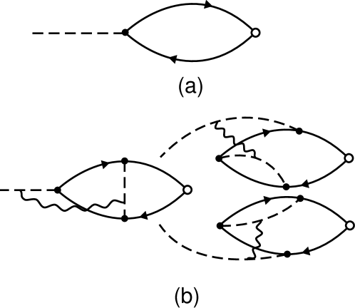
Figure 6: Representation of contributions to the correlation function in (56) in the diagrammatic approach of Appendix C; the diagram in (a) is the zeroth order result, while (b) contains diagrams of order $\gamma_{0}^{2}g$. The wavy line is the interaction $g_{0}$ and other conventions are as described in Fig 5.

This leading term evaluates at $T=0$ and $s=s_{c}$ to

$$\gamma_{0}S(S+1)\int\frac{d^{d}k}{(2\pi)^{d}}\frac{e^{ikx}}{k^{2}}.$$ (57)

Let us first consider corrections to (57) from interactions involving only the boundary coupling $\gamma_{0}$. It is easy to see that the diagrams for these have interactions along the impurity spin loop that are in one-to-one correspondence with those appearing in the evaluation of the two-point $n_{\alpha}$ correlator; these are shown in Figs 5, 11, 12 and lead to (51). However, such diagrams are obviously associated with the wavefunction renormalization, $Z^{\prime}$, of $n_{\alpha}$. So there are no contributions to the coupling constant renormalization, $Z_{\gamma}$, from the boundary interactions alone; this leads to the important result

$$\mbox{$Z_{\gamma}=1$ at $g=0$}.$$ (58)

Next, we consider interference between the bulk interaction, $g_{0}$, and the boundary interaction, $\gamma_{0}$. Now there are contributions which are specifically associated with the renormalization of $\gamma_{0}$ and these are shown in Fig 6b. Evaluating the graphs of Fig 6b at $T=0$ and $s=s_{c}$ as described in Appendix C, we obtain the following contribution to the correlator in (56)

$$-\frac{g_{0}\gamma_{0}^{3}}{6}S(S+1)\int\frac{d^{d}k}{(2\pi)^{d}}\frac{e^{ikx}}{k^{2}}\left(S(S+1)-\frac{1}{3}\right)$$

$$\quad\times\int\frac{d^{d}k_{1}}{(2\pi)^{d}}\frac{d^{d}k_{2}}{(2\pi)^{d}}\frac{1}{k_{1}^{2}k_{2}^{2}(k+k_{1}+k_{2})^{2}}.$$ (59)

After determining, by standard methods, the residue of the pole in $\epsilon$ associated with the integral in (59), we can write down the coupling constant renormalization

$$Z_{\gamma}=1+\frac{\pi^{2}[S(S+1)-1/3]}{6\epsilon}g\gamma^{2}+\cdots.$$ (60)

The above result for $Z_{\gamma}-1$ is smaller by a factor of 3 from that quoted earlier by us Science , and this corrects a numerical error in our computation. This correction also leads to corresponding minor changes in (65), (66), (68) and (125) below.

We now have all the ingredients to determine the final renormalization factor $Z^{\prime}$. Using the definitions (55) in (51), along with the result (60), and demanding that all poles in $\epsilon$ cancel, we obtain

$$Z^{\prime}=1-\frac{2\gamma^{2}}{\epsilon}+\frac{\gamma^{4}}{\epsilon}.$$ (61)

Now the RG beta-functions can be obtained by standard manipulations bgz . For the bulk coupling $g$ we obtain from the definition (52) and the values (54), the known result

$$\beta(g)\equiv\mu\frac{dg}{d\mu}\bigg{|}_{g_{0}} = -\epsilon g\left(1+\frac{d\ln Z_{4}}{d\ln g}-2\frac{d\ln Z}{d\ln g}\right)^{-1}$$ (62)

$$= -\epsilon g+\frac{11g^{2}}{6}-\frac{23g^{3}}{12}.$$

Similarly, we can obtain the beta-function for the boundary coupling $\gamma$ defined as

$$\beta(\gamma)=\mu\frac{d\gamma}{d\mu}\bigg{|}_{g_{0},\gamma_{0}}.$$ (63)

Taking the $\mu$ derivative of the second equation in (55) at fixed bare couplings $g_{0}$, $\gamma_{0}$, we get

$$-\frac{\epsilon}{2} = \beta(\gamma)\frac{\partial\ln Z_{\gamma}}{\partial\gamma}+\beta(g)\frac{\partial\ln Z_{\gamma}}{\partial g}-\frac{\beta(\gamma)}{2}\frac{\partial\ln Z^{\prime}}{\partial\gamma}$$ (64)

$$- \frac{\beta(g)}{2}\frac{\partial\ln Z^{\prime}}{\partial g}-\frac{\beta(g)}{2}\frac{d\ln Z}{dg}+\frac{\beta(\gamma)}{\gamma}$$

Solving (64) using (54,60,61,62) we obtain to the order we are working

$$\beta(\gamma)=-\frac{\epsilon\gamma}{2}+\gamma^{3}-\gamma^{5}+\frac{5g^{2}\gamma}{144}+\frac{g\gamma^{3}\pi^{2}}{3}[S(S+1)-1/3];$$ (65)

the first two terms in this beta-function agree with the earlier results of Smith and Si si and Sengupta Sengupta . The beta-functions (62) and (65) have infra-red stable fixed points at

$$g^{\ast} = \frac{6\epsilon}{11}+\frac{414\epsilon^{2}}{1331}$$

$$\gamma^{\ast 2} = \frac{\epsilon}{2}+\epsilon^{2}\left(\frac{29}{121}-\frac{\pi^{2}}{11}[S(S+1)-1/3]\right)$$ (66)

These fixed point values control all of the universal physical quantities computed in this paper. In particular, we can now immediately obtain the exponents $\eta$ and $\eta^{\prime}$. The value of $\eta$ is, of course, known previously, and is given by

$$\eta=\mu\frac{d\ln Z}{d\mu}\bigg{|}_{g=g^{\ast}} = \beta(g)\frac{d\ln Z}{dg}\bigg{|}_{g=g^{\ast}}$$ (67)

$$= \frac{5\epsilon^{2}}{242}.$$

For the new boundary anomalous dimension $\eta^{\prime}$ we have

$$\eta^{\prime} = \mu\frac{d\ln Z^{\prime}}{d\mu}\bigg{|}_{g=g^{\ast},\gamma=\gamma^{\ast}}$$ (68)

$$= \beta(\gamma)\frac{\partial\ln Z^{\prime}}{\partial\gamma}+\beta(g)\frac{\partial\ln Z^{\prime}}{\partial g}\bigg{|}_{g=g^{\ast},\gamma=\gamma^{\ast}}$$

$$= \epsilon-\epsilon^{2}\left(\frac{5}{242}+\frac{2\pi^{2}}{11}[S(S+1)-1/3]\right).$$

This exponent $\eta^{\prime}$ controls the decay of the two-point $n_{\alpha}$ correlations at the $T=0$ critical point at $s=s_{c}$, as in (33). For $s>s_{c}$ in the $T=0$ quantum paramagnet, $\eta^{\prime}$ determines the impurity static moment, as was asserted in (36) and (37). These facts are demonstrated explicitly in perturbation theory in Appendix D.

We close this section by mentioning an interesting bi-product of our analysis: we will obtain an exact exponent for some simpler models considered earlier in the literature. Consider the fixed point of the beta-functions above with $g=0$ and $\gamma=\widetilde{\gamma}^{\ast}\neq 0$, so that the bulk fluctuations of the $\phi_{\alpha}$ are described by a Gaussian theory. Such a fixed point is unstable in the infra-red to the fixed point we have already considered, and so does not generically describe impurities in any antiferromagnet. Nevertheless, it is an instructive model to study, and closely related models appear in mean-field theories of quantum spin glasses SY2 . The fixed point value of $\widetilde{\gamma}^{\ast 2}$ can of course be easily obtained from (65) to second order in $\epsilon$–this value will have corrections at all orders in $\epsilon$, and an exact determination does not seem to be possible. Even so, we can obtain an exact result for $\eta^{\prime}$. This is a consequence of the identity (58). Using this result, and the fact that all $g$ derivatives can be neglected at $g=0$, the expressions (64) and (68) simplify to

$$\beta(\gamma) = -\frac{\epsilon\gamma}{2}\left(1-\frac{1}{2}\frac{\partial\ln Z^{\prime}}{\partial\ln\gamma}\right)^{-1}$$

$$\eta^{\prime} = \beta(\gamma)\frac{\partial\ln Z^{\prime}}{\partial\gamma}\bigg{|}_{\gamma=\widetilde{\gamma}^{\ast}}.$$ (69)

It now follows immediately from the fact that $\beta(\widetilde{\gamma}^{\ast})=0$, that

$$\eta^{\prime}=\epsilon$$ (70)

exactly at the $g=0$, $\gamma=\widetilde{\gamma}^{\ast}$ fixed point.

II.2 Spin correlations in the paramagnet

The results in this section will be limited to $s\geq s_{c}$, i.e., the right half of Fig 3.

We will be interested in numerous different linear response functions of $\mathcal{S}_{\text{b}}+\mathcal{S}_{\text{imp}}$. To discuss these in some generality, we extend the actions by coupling them to a number of different external fields: in $\mathcal{S}_{\text{b}}$ we make the transformation

$$(\partial_{\tau}\phi_{\alpha})^{2}\rightarrow(\partial_{\tau}-i\epsilon_{\alpha\beta\gamma}H_{\text{u}\beta}(x)\phi_{\gamma})^{2}-H_{\text{s}\alpha}(x)\phi_{\alpha},$$ (71)

while we add to $\mathcal{S}_{\text{imp}}$ the coupling

$$-S\int d\tau H_{\text{imp},\alpha}n_{\alpha}(\tau).$$ (72)

The field $H_{\text{u}}(x)$ is an external magnetic field which varies as a function of $x$ only on a scale much larger than the lattice spacing of the underlying antiferromagnet. In contrast, $H_{\text{s}}(x)$ is a staggered magnetic field which couples to the antiferromagnetic order parameter—so it oscillates rapidly on the lattice scale, but has an envelope which is slowly varying; such fields cannot be imposed directly in the laboratory, but associated response function can be measured in NMR and neutron scattering measurements. Finally $H_{\text{imp}}$ is the magnetic field at the location of the impurity. So a space-independent, uniform magnetic field $H$ applied to the antiferromagnet corresponds to $H_{\text{u}}(x)=H$, $H_{\text{s}}=0$, and $H_{\text{imp}}(x)=H$. We have also taken all fields to be time independent for simplicity - it is not difficult to extend our approach to dynamic response functions with time-dependent fields.

We can now consider a total of six different response function to these external fields. We tabulate below results for these response functions obtained in bare perturbation theory, to lowest non-trivial order. The computation is performed by the methods of Appendix C and is quite straightforward–we do not explicitly show the Feynman diagrams associated with these results. The results will subsequently be interpreted using the RG formulated in Section II.1.

$$\chi_{\text{u},\text{u}}(x,x^{\prime}) \equiv \frac{T}{3}\frac{\delta^{2}\ln Z}{\delta H_{\text{u}\alpha}(x)\delta H_{\text{u}\alpha}(x^{\prime})}$$

$$= \delta^{d}(x-x^{\prime})\frac{2S(S+1)}{3T}\gamma_{0}^{2}TG^{2}(x)$$

$$\chi_{\text{u},\text{imp}}(x) \equiv \frac{T}{3}\frac{\delta^{2}\ln Z}{\delta H_{\text{u}\alpha}(x)\delta H_{\text{imp},\alpha}}$$

$$= \frac{S(S+1)}{3T}\gamma_{0}^{2}\int\frac{d^{d}k_{1}}{(2\pi)^{d}}\frac{d^{d}k_{2}}{(2\pi)^{d}}\frac{e^{i(k_{1}-k_{2})x}}{\varepsilon_{k_{1}}\varepsilon_{k_{2}}}$$

$$\times\bigg{[}\frac{(\varepsilon_{k_{2}}\coth(\varepsilon_{k_{1}}/2T)-\varepsilon_{k_{1}}\coth(\varepsilon_{k_{2}}/2T))}{(\varepsilon_{k_{2}}^{2}-\varepsilon_{k_{1}}^{2})}$$

$$\qquad-\frac{2T}{\varepsilon_{k_{1}}\varepsilon_{k_{2}}}\bigg{]}$$

$$\chi_{\text{u},\text{s}}(x,x^{\prime}) \equiv \frac{T}{3}\frac{\delta^{2}\ln Z}{\delta H_{\text{u}\alpha}(x)\delta H_{\text{s}\alpha}(x^{\prime})}$$

$$= \gamma_{0}\chi_{\text{u},\text{imp}}(x)G(x^{\prime})$$

$$\chi_{\text{imp},\text{imp}} \equiv \frac{T}{3}\frac{\delta^{2}\ln Z}{\delta H_{\text{imp},\alpha}\delta H_{\text{imp},\alpha}}$$

$$= \frac{S(S+1)}{3T}\left(1-2\gamma_{0}^{2}\mathcal{F}\right)$$

$$\chi_{\text{s},\text{imp}}(x) \equiv \frac{T}{3}\frac{\delta^{2}\ln Z}{\delta H_{\text{s}\alpha}(x)\delta H_{\text{imp},\alpha}}$$

$$= -2\frac{S(S+1)}{3T}\gamma_{0}^{3}G(x)\mathcal{F}$$

$$\chi_{\text{s},\text{s}}(x,x^{\prime}) \equiv \frac{T}{3}\frac{\delta^{2}\ln Z}{\delta H_{\text{s}\alpha}(x)\delta H_{\text{s}\alpha}(x^{\prime})}$$ (73)

$$= \frac{S(S+1)}{3T}\gamma_{0}^{2}G(x)G(x^{\prime})$$

where

$$\varepsilon_{k} \equiv (k^{2}+m^{2})^{1/2}\,,$$

$$G(x) \equiv \int\frac{d^{d}k}{(2\pi)^{d}}\frac{e^{ikx}}{\varepsilon_{k}^{2}}\,,$$

$$\mathcal{F} \equiv \int\frac{d^{d}k}{(2\pi)^{d}}\left(\frac{\coth(\varepsilon_{k}/2T)}{2\varepsilon_{k}^{3}}-\frac{T}{\varepsilon_{k}^{4}}\right).$$ (74)

The prefactors of $1/3$ in (73) merely perform the rotational averaging over the directions in spin space. It is important to note that we have only included impurity related contributions in the above results: the portions of the susceptibilities which are a property of the bulk theory, $\mathcal{S}_{\text{b}}$, alone have been dropped as they were considered in earlier work.

We will now combine these results into various observable correlators and discuss their scaling properties.

II.2.1 Impurity susceptibility

First, let us consider the impurity susceptibility, $\chi_{\text{imp}}$, defined in (11). This is related to the expressions in (73) by

$$\chi_{\text{imp}}\equiv\chi_{\text{imp},\text{imp}}+2\int\!d^{d}x\chi_{\text{u},\text{imp}}(x)$$

$$\qquad\qquad\qquad+\int\!d^{d}xd^{d}x^{\prime}\chi_{\text{u},\text{u}}(x,x^{\prime})$$

$$\!\!\!\!\!\!\!\!\!=\frac{S(S+1)}{3T}\left[1+\frac{\gamma_{0}^{2}}{2T}\!\!\int\!\!\frac{d^{d}k}{(2\pi)^{d}}\frac{1}{\varepsilon_{k}^{2}\sinh^{2}(\varepsilon_{k}/2T)}\right].$$ (75)

An important property of the above expression is that as $T\rightarrow 0$ for $s>s_{c}$, the term of order $\gamma_{0}^{2}$ is exponentially suppressed and the response reduces to that of a free spin $S$: this indicates, as expected, that the total magnetic moment associated with the impurity is precisely $S$ in paramagnetic phase. This last fact can also be established directly by computing the magnetization in the presence of a finite field $H$ at $T=0$; this can be done to all orders in $H$ by the methods to be developed in Section II.3, and the result (120) holds—we will not present the details here.

Next, we examine the behavior of $\chi_{\text{imp}}$ as $s$ approaches $s_{c}$ from above. The momentum integral in (75) is exponentially convergent, and so there are no poles in $\epsilon$. This implies, as expected from the conservation of total spin, that $\chi_{\text{imp}}$ acquires no anomalous dimensions, and (75) can be written in the scaling form

$$\chi_{\text{imp}}=\frac{1}{T}\Phi_{\text{imp}}\left(\frac{\Delta}{T}\right),$$ (76)

with $\Phi_{\text{imp}}$ a universal scaling function. The latter can be evaluated from (75) by setting $\gamma=\gamma^{\ast}$, and by using the crossover function for $m$ in Ref. ss, . Let us consider such an evaluation explicitly at $s=s_{c}$. Then, from (47), $m$ is proportional to $T$, but with the proportionality constant of order $\epsilon^{1/2}$. It is therefore tempting, to leading order in $\epsilon$, to simply set $m=0$ in the integrand in (75). However, this leads to trouble—the integrand in (75) is infrared singular, and behaves like $1/(k^{2}+m^{2})^{2}$ at low momentum. So we have to keep a finite value of $m$, and the correction of order in $\gamma_{0}^{2}$ in (75), which is superficially of order $\epsilon$, turns out to be of order $\epsilon^{1/2}$. By such a calculation, we find that at $s=s_{c}$, $\chi_{\text{imp}}$ takes the form (31), with

$$\mathcal{C}_{1}=\frac{S(S+1)}{3}\left[1+\left(\frac{33\epsilon}{40}\right)^{1/2}+O\left(\epsilon\right)\right].$$ (77)

Actually, it is possible to also obtain the $O(\epsilon)$ contribution above without too much additional difficulty. To do this, we have to identify only the contributions to $\chi_{\text{imp}}$ at order $\gamma_{0}^{4}$ and $\gamma_{0}^{2}g_{0}$, which are infrared singular enough to reduce the expression from superficial order $\epsilon^{2}$ to order $\epsilon$. It turns out that there is only a single graph for $\chi_{\text{u},\text{u}}$ which can accomplish this, and it contributes

$$-\frac{S(S+1)}{3}\frac{5u_{0}\gamma_{0}^{2}}{3}\left[\int\frac{d^{d}k}{(2\pi)^{d}}\frac{1}{\varepsilon_{k}^{4}}\right]^{2}$$ (78)

to $\chi_{\text{imp}}$. Evaluating (78), and also identifying the $O(\epsilon)$ contribution from (75), we correct (77) to

$$\mathcal{C}_{1}=\frac{S(S+1)}{3}\left[1+\left(\frac{33\epsilon}{40}\right)^{1/2}-\frac{7\epsilon}{4}+O\left(\epsilon^{3/2}\right)\right].$$ (79)

II.2.2 Local susceptibility

Second, consider the response, at or close to the impurity site, to a local magnetic field applied near the impurity site. This is usually denoted by $\chi_{\text{loc}}$ and could be measured in a muon spin resonance experiment; we define it by

$$\chi_{\text{loc}}=Z^{\prime-1}\chi_{\text{imp},\text{imp}}.$$ (80)

We have inserted a prefactor of $Z^{\prime-1}$ because $\chi_{\text{imp},\text{imp}}$ is the two-point correlator of the $n_{\alpha}$, and this acquires a field renormalization factor $Z^{\prime-1/2}$ in (55). It is now easy to verify from (73) and (61) that the poles in $\epsilon$ do cancel, and that (80) can be written in the form

$$\chi_{\text{loc}}=\frac{\mu^{-\eta^{\prime}}}{T^{1-\eta^{\prime}}}\Phi_{\text{loc}}\left(\frac{\Delta}{T}\right).$$ (81)

Again $\Phi_{\text{loc}}$ is a universal scaling function; it reaches a constant value at zero argument and so $\chi_{\text{loc}}$ diverges as $T^{-1+\eta^{\prime}}$ at $s=s_{c}$. For $s>s_{c}$, we see from (73) that $\chi_{\text{loc}}\sim 1/T$ as $T\rightarrow 0$. We can consider this as arising from the overlap of the impurity moment with the total, freely fluctuating, moment of $S$ that was considered below (75), and so write

$$\lim_{T\rightarrow 0}\chi_{\text{loc}}=\frac{S(S+1)}{3T}m_{\text{imp}}^{2}\quad;\quad s>s_{c}.$$ (82)

From the expressions in (73), we deduce

$$m_{\text{imp}}=Z^{\prime-1/2}\left[1-\frac{\gamma_{0}^{2}}{2}\int\!\!\frac{d^{d}k}{(2\pi)^{d}}\frac{1}{\varepsilon_{k}^{3}}\right].$$ (83)

It can now be checked that this value for $m_{\text{imp}}$ agrees precisely with that computed from the definition (36) – this is shown in Appendix D, where $m_{\text{imp}}^{2}$ evaluates to (211). Also this last result, or (81), show that (37) is obeyed with $\eta^{\prime}=\epsilon$. Alternatively, we can use the methods of Section II.3 to compute the $T=0$ impurity magnetization in the presence of a finite field $H$, to all orders in $H$, and the result agrees with (83).

II.2.3 Knight shift

Finally, we measure the space-dependent response to a uniform magnetic field, $H$. This can be measured in a NMR experiment as a Knight shift, as was done in Refs. alloul2, ; julien, , with the results indicated in Fig 1. We are considering linear response in $H$, and so such results are implicitly valid for $H\ll T$. However, experiments alloul2 ; julien are often in a regime where $H$ is of order $T$, and so it is useful to go beyond linear response, and obtain the full $H/T$ dependence of the Knight shift. We will show that this can be done using some simple arguments in the spin-gap regime ($s>s_{c}$) with $T,H\ll\Delta$, but $H/T$ arbitrary: from the knowledge of the linear response in $H$, the entire $H/T$ dependence can be reconstructed. In the quantum critical region ($T\gg\Delta$, $s\geq s_{c}$) we will be satisfied by exploring $H\ll T$ in linear response; in the opposite limit, the host antiferromagnet undergoes a phase transition to a canted stateconserve ; troyerss induced by the applied field at $H\sim T$, and we wish to avoid such complications here.

We can identify three important components of a Knight shift: (i) $K_{\text{imp}}$, the Knight shift of a nucleus at, or very close to, the impurity site; (ii) $K_{\text{s}}(x)$, the envelope of a Knight shift which oscillates rapidly with the orientation of the antiferromagnetic order parameter, (i.e., as $\cos({\bf Q}.x))$; and (iii) $K_{\text{u}}(x)$, the uniform component of the Knight shift away from the impurity site. We will consider these three in turn. We measure the Knight shift as simply the mean electronic moment at a particular location, and will drop the factor of the electron-nucleus hyperfine coupling.

(a) $K_{\text{imp}}$

We define $K_{\text{imp}}$ by

$$K_{\text{imp}}=Z^{\prime-1/2}\bigg{[}\chi_{\text{imp},\text{imp}}+\int\!\!d^{d}x\chi_{\text{u},\text{imp}}(x)\bigg{]}H$$

$$\quad=Z^{\prime-1/2}\frac{S(S+1)}{3T}\bigg{[}1-\gamma_{0}^{2}\int\!\!\frac{d^{d}k}{(2\pi)^{d}}\bigg{(}\frac{\coth(\varepsilon_{k}/2T)}{2\varepsilon_{k}^{3}}$$

$$\qquad\qquad\qquad-\frac{1}{4T\varepsilon_{k}^{2}\sinh^{2}(\varepsilon_{k}/2T)}\bigg{)}\bigg{]}H.$$ (84)

This has a renormalization factor of only $Z^{\prime-1/2}$ because it is the correlator of $n_{\alpha}$ with the total magnetization, and the latter conserved quantity requires no renormalization. There is an overall factor of $H$ because the magnetization is induced by the external field, and we are considering linear response. As for (81), it can be verified from (73) and (61) that the poles in $\epsilon$ cancel, and the result is of the form

$$K_{\text{imp}}=\frac{\mu^{-\eta^{\prime}/2}}{T^{1-\eta^{\prime}/2}}H\Phi_{K_{\text{imp}}}\left(\frac{\Delta}{T}\right).$$ (85)

The scaling function $\Phi_{K_{\text{imp}}}$ reaches a constant value at zero argument, and so $K_{\text{imp}}$ diverges as $T^{-1+\eta^{\prime}/2}$ at $s=s_{c}$.

For $s>s_{c}$, $K_{\text{imp}}\sim 1/T$ as $T\rightarrow 0$, and by the analog of the arguments associated with (82) we can now write

$$\lim_{T\rightarrow 0}K_{\text{imp}}=\frac{S(S+1)}{3T}m_{\text{imp}}H\quad;\quad s>s_{c};$$ (86)

the resulting value for $m_{\text{imp}}$ agrees with (83). We can extend (86) to beyond linear response in $H$ for $T,H\ll\Delta$ by realizing that the important thermal excitations in such a regime are simply those of the free spin in the external field; so the prefactor of the free spin susceptibility in (86) is simply the component of the free spin wavefunction near the impurity. We can expect that the same prefactor applies for arbitrary $H/T$, and so the general response is the same prefactor times the free spin magnetization in a field $H$ at temperature $T$; this generalizes (86) to

$$K_{\text{imp}}=m_{\text{imp}}SB_{S}(SH/T)\quad;\quad H,T\ll\Delta,$$ (87)

where $B_{S}(y)$ is the familiar Brillouin function for spin $S$:

$$B_{S}(y)=\frac{2S+1}{2S}\coth\left(\frac{2S+1}{2S}y\right)-\frac{1}{2S}\coth\left(\frac{1}{2S}y\right);$$ (88)

note that $B_{S}(y)\sim y$ for small $y$, and $B_{S}(y\rightarrow\infty)=1$. Naturally, (87) reduces to (86) for $H\rightarrow 0$. For large $H/T$, the impurity Knight shift is $S$ times the impurity moment $m_{\text{imp}}$.

(b) $K_{\text{s}}$

For the staggered Knight shift, we have the expression

$$K_{\text{s}}(x)=Z^{-1/2}\left[\chi_{\text{s},\text{imp}}(x)+\int\!\!d^{d}x^{\prime}\chi_{\text{u},\text{s}}(x^{\prime},x)\right]H.$$ (89)

Notice that now we only have the field scale renormalization of the bulk theory, as we are considering a correlator of $\phi_{\alpha}(x)$ with the total conserved spin. To the order we are working, we can simply set $Z=1$, and then the expressions in (73) yield

$$K_{\text{s}}(x)=\frac{S(S+1)}{3T}G(x)\bigg{[}\gamma_{0}-\gamma_{0}^{3}\int\frac{d^{d}k}{(2\pi)^{d}}\bigg{(}$$

$$\quad\frac{\coth(\varepsilon_{k}/2T)}{2\varepsilon_{k}^{3}}-\frac{1}{4T\varepsilon_{k}^{2}\sinh^{2}(\varepsilon_{k}/2T)}\bigg{)}\bigg{]}H.$$ (90)

Upon using (55) and (61) it can be verified that the above is free of poles in $\epsilon$, and the result is of the form

$$K_{\text{s}}(x)=\frac{\mu^{-\eta/2}}{T^{(3-d-\eta)/2}}H\Phi_{K_{\text{s}}}\left(\frac{\Delta}{T},Tx\right),$$ (91)

with $\Phi_{K_{\text{s}}}$ a universal function, as is expected from general scaling arguments. At the approximation we have computed things, $\eta=0$, and $K_{\text{s}}(x)\sim(H/T)G(x)[\mbox{Max}(T,\Delta)]^{\epsilon/2}$.

As for $K_{\text{imp}}$, we can generalize (91) to obtain the non-linear response in $H$ in the spin gap regime ($H,T\ll\Delta$). We first identify a local staggered moment as in (86)

$$\lim_{T\rightarrow 0}K_{\text{s}}(x)=\frac{S(S+1)}{3T}\frac{\langle\phi_{z}(x)\rangle}{S}H\quad;\quad s>s_{c};$$ (92)

we have identified the staggered moment as proportional to the expectation value of the antiferromagnetic order in an applied field in the $z$ direction, and the factor of $1/S$ follows because we have absorbed a factor of $S$ in defining the free moment of which $\langle\phi_{z}\rangle$ is an envelope. From (90) we obtain immediately

$$\langle\phi_{z}(x)\rangle=SG(x)\bigg{[}\gamma_{0}-\gamma_{0}^{3}\int\!\!\frac{d^{d}k}{(2\pi)^{d}}\frac{1}{2\varepsilon_{k}^{3}}\bigg{]};$$ (93)

this expression for $\langle\phi_{z}(x)\rangle$ can also be obtained by the methods of Section II.3 by computing the staggered magnetization in the presence of a finite field at $T=0$. The factor in the square brackets, after using (55) and (61), is free of poles in $\epsilon$, and evaluates to order $\Delta^{\epsilon/2}$ at the fixed point value for $\gamma$. Because of the $G(x)$ factor, $\langle\phi_{z}(x)\rangle$ decays exponentially for large $x$, and we will consider its small $x$ behavior shortly. To obtain the non-linear response we now have the analog of (87):

$$K_{\text{s}}(x)=\langle\phi_{z}(x)\rangle B_{S}(SH/T)\quad;\quad H,T\ll\Delta.$$ (94)

So at large $H/T$, the staggered Knight shift simply measures the space-dependent antiferromagnetic moment induced by the impurity spin.

We examine the behaviors of $K_{\text{s}}(x)$ and $\langle\phi_{z}(x)\rangle$ for small $x$; these are specified by the operator product expansion in (38):

$$\lim_{|x|\rightarrow 0}\langle\phi_{z}(x)\rangle\sim\frac{m_{\text{imp}}}{|x|^{(d-1+\eta-\eta^{\prime})/2}}\,.$$ (95)

where $m_{\text{imp}}$ was obtained in (86); a similar result holds for the Knight shift in linear response in $H$ but all $T$:

$$\lim_{x\rightarrow 0}K_{\text{s}}(x)\sim\frac{K_{\text{imp}}}{|x|^{(d-1+\eta-\eta^{\prime})/2}}.$$ (96)

Provided the value of $\eta^{\prime}$ is such that $d-1+\eta-\eta^{\prime}>0$ (which we definitely expect), the staggered Knight shift will increase as one approaches the impurity, as seen in Refs. alloul2, ; alloul2a, ; julien, . Indeed, all of the results of this subsection are qualitatively consistent with the trends in Fig 1.

(c) $K_{\text{u}}$

The remaining uniform Knight shift is given by

$$K_{\text{u}}(x)=\left[\chi_{\text{u},\text{imp}}(x)+\int\!\!d^{d}x^{\prime}\chi_{\text{u},\text{u}}(x^{\prime},x)\right]H.$$ (97)

Now no renormalization factors are necessary because this is a correlator of the conserved spin of the bulk theory with the conserved spin of the total theory, and neither of them acquire any anomalous dimensions. Evaluation of (97) using (73) gives

$$K_{\text{u}}(x)=\frac{S(S+1)}{3T}\gamma_{0}^{2}\int\frac{d^{d}k_{1}}{(2\pi)^{d}}\frac{d^{d}k_{2}}{(2\pi)^{d}}\frac{e^{i(k_{1}-k_{2})x}}{\varepsilon_{k_{1}}\varepsilon_{k_{2}}}$$

$$\times\frac{(\varepsilon_{k_{2}}\coth(\varepsilon_{k_{1}}/2T)-\varepsilon_{k_{1}}\coth(\varepsilon_{k_{2}}/2T))}{(\varepsilon_{k_{2}}^{2}-\varepsilon_{k_{1}}^{2})}H.$$ (98)

At the fixed point of the beta-functions, this is of the universal scaling form

$$K_{\text{u}}(x)=T^{d-1}H\Phi_{K_{\text{u}}}\left(\frac{\Delta}{T},Tx\right).$$ (99)

As in the staggered case, we can go beyond linear response in $H$ for $H,T\ll\Delta$. Then, following (92), we define a uniform magnetization $\langle L_{z}\rangle(x)\rangle$ by

$$\lim_{T\rightarrow 0}K_{\text{u}}(x)=\frac{S(S+1)}{3T}\frac{\langle L_{z}(x)\rangle}{S}H\quad;\quad s>s_{c},$$ (100)

and an expression for $\langle L_{z}(x)\rangle$ follows from (98). The non-linear response, generalizing (94) is

$$K_{\text{u}}(x)=\langle L_{z}(x)\rangle B_{S}(SH/T)\quad;\quad H,T\ll\Delta.$$ (101)

As before, the small $x$ behavior of the scaling function is controlled by the operator product expansion (38):

$$\lim_{|x|\rightarrow 0}\langle L_{z}(x)\rangle\sim\frac{m_{\text{imp}}}{|x|^{d-\eta^{\prime}/2}},$$ (102)

and

$$\lim_{x\rightarrow 0}K_{\text{u}}(x)\sim\frac{K_{\text{imp}}}{|x|^{d-\eta^{\prime}/2}}.$$ (103)

II.3 Spin correlations in the Néel state

We consider impurity properties when spin rotation invariance has been broken in the host antiferromagnet for $s<s_{c}$. We will restrict our attention to $T=0$.

The field $\phi_{\alpha}$ has an average orientation which we take in the $z$ direction. To lowest order in $g_{0}$ this expectation value is

$$\langle\phi_{\alpha}(x)\rangle=\left(\frac{-6s}{g_{0}}\right)^{1/2}\delta_{\alpha,z};$$ (104)

there is no dependence on $x$ at this order. We will consider corrections to this result in renormalized perturbation theory. In preparation, we quote some additional properties of the host antiferromagnet. We will need the value of the critical coupling to leading order in $s_{c}$ ss

$$s_{c}=-\frac{5g_{0}}{6}\int\frac{d\omega}{2\pi}\int\frac{d^{d}k}{(2\pi)^{d}}\frac{1}{k^{2}+\omega^{2}}.$$ (105)

We also define a parameter $\tilde{s}_{0}$ measuring the deviation from the critical point

$$s=s_{c}+\tilde{s}_{0}.$$ (106)

Associated with this is a renormalized $\tilde{s}$ and a bulk renormalization factor $Z_{2}$

$$\tilde{s}_{0}=\tilde{s}\frac{Z_{2}}{Z},$$ (107)

and to lowest order in $g$ we havebgz

$$Z_{2}=1+\frac{5g}{6\epsilon}.$$ (108)

The ordering in the host antiferromagnet produces an effective field on the impurity spin, and so its fluctuations are anisotropic. In principle, these can be computed order-by-order in $\gamma_{0}$ by the perturbative methods discussed in Appendix C. However, spin anisotropy leads to a proliferation in the number of diagrams, and we found it more convenient to use in alternative approach. Indeed, the broken spin rotation invariance implies that traditional methods developed for ordered magnets can be applied here: we used the Dyson-Maleev representation for the impurity spin dyson ; maleev ; abp . A potential problem with the Dyson-Maleev representation is that it is designed to obtain results order-by-order by an expansion in $1/S$, while all our results so far have been exact as a function of $S$. However, it turns out that, at $T=0$, the Feynman graph expansion of the Dyson-Maleev representation of our problem remains a perturbation theory in $g_{0}$ and $\gamma_{0}$: to each order in these parameters, the results are exact as a function of $S$. This is a consequence of there being only a small number of Dsyon-Maleev bosons in every intermediate state in the perturbation theory, and these can couple only through a limited number of non-linear interactions. In contrast, at $T>0$, the Dyson-Maleev perturbation theory sums over an infinite number of intermediate states with an arbitrary number of bosons, and the results are then no longer exact as a function of $S$; in this case the methods of Appendix C should be used, as they remain exact even for $T>0$. Our interest here is only in $T=0$, and so we will use the more convenient Dyson-Maleev method–it has the advantage of using canonical bosons and so permits use of standard time-ordered diagrams, the Dyson theorem, and automatic cancellation of disconnected diagrams.

Let us introduce the Dyson-Maleev formulations. We label the states of the impurity spin by the occupation number of a canonical boson, $b$. The spin-operator is given by

$$Sn_{z} = S-b^{\dagger}b$$

$$S(n_{x}-in_{y}) = \sqrt{2S}b^{\dagger}$$

$$S(n_{x}+in_{y}) = \sqrt{2S}\left(b-\frac{b^{\dagger}bb}{2S}\right).$$ (109)

Notice that the representation does not appear to respect the Hermiticity of the spin operators; this is because a similarity transformation has been performed on the Hilbert space—we refer the reader to the literature for more discussion on this point. It is also convenient to define a ‘circularly’ polarized combination of the bulk field $\phi_{\alpha}$, and to shift the longitudinal component from the mean value in (104):

$$\psi = (\phi_{x}+i\phi_{y})/\sqrt{2}$$

$$\phi_{z} = \left(\frac{-6s}{g_{0}}\right)^{1/2}+\widetilde{\phi}_{z}$$ (110)

Now $\mathcal{S}_{\text{imp}}$ in (13) takes the form (we only have a single impurity at $r=0$ and have dropped the sum over $r$)

$$\mathcal{S}_{\text{imp}} = \int_{0}^{\beta}\!\!d\tau\bigg{[}b^{\dagger}\left(\frac{d}{d\tau}+\gamma_{0}\sqrt{-6s/g_{0}}\right)b$$ (111)

$$\quad-\gamma_{0}\widetilde{\phi}_{z}(S-b^{\dagger}b)$$

$$\quad-\gamma_{0}\sqrt{S}\left(b^{\dagger}\psi+\psi^{\ast}b-\frac{\psi^{\ast}b^{\dagger}bb}{2S}\right)\bigg{]},$$

where it is understood that $\widetilde{\phi}_{z}$ and $\psi$ are evaluated at $x=0$ in the above. Notice that, at zeroth order, the $b$ bosons have finite energy gap of $\gamma_{0}\sqrt{-6s/g_{0}}$—it is this gap which stabilizes the perturbation theory and permits evaluation of results exact in $S$ at each order in $\gamma_{0}$ and $g_{0}$. For completeness, we also quote the bulk action $\mathcal{S}_{\text{b}}$ in (4) in this representation:

$$\mathcal{S}_{\text{b}}=\int\!\!d^{d}x\int_{0}^{\beta}\!\!d\tau\bigg{[}\frac{1}{2}\left((\partial_{\tau}\widetilde{\phi}_{z})^{2}+c^{2}(\nabla_{x}\widetilde{\phi}_{z})^{2}-2s\phi_{z}^{2}\right)$$

$$\qquad+|\partial_{\tau}\psi|^{2}+c^{2}|\nabla_{x}\psi|^{2}+\left(\frac{-sg_{0}}{6}\right)^{1/2}\left(\widetilde{\phi}_{z}^{3}+\widetilde{\phi}_{z}|\psi|^{2}\right)$$

$$\qquad+\frac{g_{0}}{4!}\left(\widetilde{\phi}_{z}^{4}+4\widetilde{\phi}_{z}^{2}|\psi|^{2}+4|\psi|^{4}\right)\bigg{]},$$ (112)

The partition function is now an unrestricted functional integral over $b(\tau)$, $\widetilde{\phi}_{z}(x,\tau)$ and $\psi(x,\tau)$ with weight $\exp(-\mathcal{S}_{\text{b}}-\mathcal{S}_{\text{imp}})$.

Computation of the perturbation theory in $\gamma_{0}$ and $g_{0}$ in above representation is a completely straightforward application of standard methods. There are a fair number of non-linear couplings, and so tabulation of all the graphs can be tedious. We will be satisfied here by simply quoting the results of perturbation theory and then providing a scaling interpretation. We consider a few different observables in the following subsections.

II.3.1 Static magnetization

We consider the static magnetization of the impurity site, and also the staggered and uniform moments in the host antiferromagnet.

First, the static magnetization of the impurity, $m_{\text{imp}}$, defined in (36). In bare perturbation theory we obtain

$$m_{\text{imp}} = \langle n_{z}\rangle=\bigg{[}1-\gamma_{0}^{2}\int\frac{d^{d}k}{(2\pi)^{d}}\int\frac{d\omega}{2\pi}$$ (113)

$$\times\frac{1}{(k^{2}+\omega^{2})(-i\omega+\gamma_{0}\sqrt{-6s/g_{0}})^{2}}\bigg{]}$$

We evaluate the integral, perform the substitutions to the renormalized couplings and fields in (52), (55), (106) and (107), use the renormalization constants in (54), (60), (61) and (108), and then expand to the appropriate order in $\epsilon$. All poles in $\epsilon$ cancel and we obtain

$$m_{\text{imp}}=1+\gamma^{2}\left(\frac{1}{2}\ln\left(\frac{-\tilde{s}}{\mu^{2}}\right)+\gamma_{E}+\frac{1}{2}\ln\left(\frac{12\gamma^{2}}{\pi g}\right)\right),$$ (114)

where $\gamma_{E}$ is the Euler-Mascheroni constant. Substituting the fixed point values $\gamma^{\ast 2}=\epsilon/2$, $g^{\ast}=6\epsilon/11$, and exponentiating we see that

$$m_{\text{imp}}\sim\left(\frac{-\tilde{s}}{\mu^{2}}\right)^{\epsilon/4}.$$ (115)

By (37) this defines the exponent $\eta^{\prime}\nu/2$, and is consistent with the leading order values $\nu=1/2$, $\eta^{\prime}=\epsilon$.

Next we turn to the spatial dependence of the static moment in the host antiferromagnet. There will be a staggered contribution to this which oscillates with the local orientation of the antiferromagnetic order, given by $\langle\phi_{z}(x)\rangle$. Evaluating the latter in perturbation theory we obtain

$$\langle\phi_{z}(x)\rangle=\gamma_{0}S\int\!\!\frac{d^{d}k}{(2\pi)^{d}}\frac{e^{ikx}}{k^{2}-2s}+\left(\frac{-6s}{g_{0}}\right)^{1/2}\bigg{[}1+$$

$$\quad\frac{g_{0}}{2}\int\!\!\frac{d^{d}k}{(2\pi)^{d}}\int\!\!\frac{d\omega}{2\pi}\frac{1}{(k^{2}+\omega^{2})(k^{2}+\omega^{2}-2s)}\bigg{]}.$$ (116)

This is evaluated by the method described below (113); again poles in $\epsilon$ cancel and we obtain

$$\langle\phi_{Rz}(x)\rangle = \left(\frac{-3\tilde{s}}{4\pi^{2}g}\right)^{1/2}\bigg{[}1+\frac{g}{4}\ln\frac{\mu^{2}}{(-2\tilde{s})}$$ (117)

$$+\gamma\sqrt{g}SF_{1}(x\sqrt{-2\tilde{s}})\bigg{]}.$$

The function $F_{1}$ has the properties

$$F_{1}(y) = \left(\frac{4\pi}{3y}\right)^{1/2}K_{1/2}(y)$$

$$\lim_{y\rightarrow 0}F_{1}(y) \sim 1/y$$

$$\lim_{y\rightarrow\infty}F_{1}(y) \sim e^{-y}/y,$$ (118)

where $K_{d/2-1}(y)$ is a modified Bessel function. After substituting fixed points values for $\gamma$ and $g$ in (117), we see that for $|x|\rightarrow\infty$, the moment has the bulk behaviorbgz ; ss $\sim(-\tilde{s})^{\beta}$ with exponent $\beta=1/2-3\epsilon/22$, as expected. In the opposing limit, the result is consistent with that expected from the operator product expansion (38), given in (95), to leading order in $\epsilon$.

A second contribution to the host static magnetization is uniform on the lattice scale—this is given by the expectation value of the magnetization, $\langle L_{z}(x)\rangle$, defined in (20). Perturbation theory yields

$$\langle L_{z}(x)\rangle = \gamma_{0}^{2}S\int\!\!\frac{d^{d}k_{1}}{(2\pi)^{d}}\frac{d^{d}k_{2}}{(2\pi)^{d}}e^{i(k_{1}+k_{2})x}\int\frac{d\omega}{2\pi}$$ (119)

$$\!\!\!\!\!\!\!\!\!\!\!\!\!\!\!\!\!\!\!\!\!\!\!\!\times\frac{-i\omega}{(\omega^{2}+k_{1}^{2})(\omega^{2}+k_{2}^{2})(-i\omega+\gamma_{0}\sqrt{-6s/g_{0}})}$$

$$= \frac{\gamma_{0}^{2}S}{2}\int\!\!\frac{d^{d}k_{1}}{(2\pi)^{d}}\frac{d^{d}k_{2}}{(2\pi)^{d}}\frac{e^{i(k_{1}+k_{2})x}}{(|k_{1}|+|k_{2}|)}$$

$$\!\!\!\!\!\!\!\!\!\!\!\!\!\!\!\!\!\!\!\!\!\!\!\!\times\frac{1}{(|k_{1}|+\gamma_{0}\sqrt{-6s/g_{0}})(|k_{2}|+\gamma_{0}\sqrt{-6s/g_{0}})}.$$

We will leave this integral in the unevaluated form above: suffice to say that $\langle L_{z}(x)\rangle$ decays to 0 at large $|x|$, while (102) holds for small $x$.

II.3.2 Response to a uniform magnetic field

In the notation introduced at the beginning of Section II.2, a uniform magnetic field corresponds to $H_{\text{u}\alpha}(x)=H_{\alpha}$, $H_{\text{imp},\alpha}=H_{\alpha}$, and $H_{\text{s}}=0$. We have to differentiate between the responses parallel and orthogonal to the bulk order parameter.

In the direction parallel to the bulk order (the $z$ direction), the symmetry of rotations about the $z$ axis is preserved, and this means that total spin is a good quantum number. Consequently, the total magnetic moment is quantizedsandvik2 precisely at $S$

$$T\frac{\delta\ln Z}{\delta H_{z}}=S.$$ (120)

It can be verified that this holds order-by-order in perturbation theory in $\gamma_{0}$ and $g_{0}$; the sensitive cancellations required to make this happen are consequences of gauge invariance. This magnetic moment is pinned to the direction of the bulk antiferromagnetic order and is not free to rotate–so unlike the situation in the paramagnet, it does not contribute a Curie susceptibility. Indeed, the direction of the bulk antiferromagnetic order is invariably pinned by very small anisotropies which are always present; in such a situation, the total impurity moment is also static, and longitudinal susceptibility is zero.

Now consider the response to a field in a direction (say $x$) transverse to the antiferromagnetic order, $\chi_{\perp}$. Such a field induces numerous additional terms in the action $\mathcal{S}_{\text{b}}+\mathcal{S}_{\text{imp}}$ which can be deduced from (71), (72), (109) and (110). We then expanded the partition function to second order in $H_{x}$ in a perturbation theory in $\gamma_{0}$ and $g_{0}$. This required a total of 22 one-loop Feynman diagrams. We will refrain from listing them here as the computations are completely standard—details of these diagrams are available from the authors. These diagrams were evaluated and expressed in terms of renormalized couplings as described below (113) using the Mathematica computer program. The final expressions were free of poles in $\epsilon$, and this was a very strong check on the correctness of the computations. At the fixed point value for $\gamma$ and $g$, the final result was

$$\chi_{\text{imp}\perp}=\frac{15S}{2\sqrt{-11\tilde{s}}}\Bigg{[}1-\frac{5\epsilon}{44}\ln\left(\frac{-\tilde{s}}{\mu^{2}}\right)$$

$$\!\!\!\!\!\!\!\!-\epsilon\left(1.00936+\frac{\pi S(3\sqrt{22}+14\pi)}{330}+\frac{7\pi^{2}S^{2}}{165}\right)\Bigg{]}.$$ (121)

Let us express this result in terms of the spin stiffness of the ordered state, $\rho_{s}$. We expect $\chi_{\text{imp}\perp}$ to scale as an inverse energy, and the parameter which sets the energy scale for general $d$ isss ; dsz

$$\widetilde{\rho_{s}}\equiv\left[\frac{2\epsilon}{11}\frac{\rho_{s}}{S_{d+1}}\right]^{1/(d-1)}.$$ (122)

The numerical factors have been chosen for convenience; note that in $d=2$ $\widetilde{\rho}_{s}$ is simply proportional to $\rho_{s}$. The $\epsilon$ expansion for $\widetilde{\rho_{s}}$ is available in Ref. ss, ; dsz, :

$$\frac{1}{\widetilde{\rho}_{s}}=\frac{1}{\sqrt{-2\tilde{s}}}\Bigg{[}1-\frac{5\epsilon}{44}\ln\left(\frac{-2\tilde{s}}{\mu^{2}}\right)+\frac{127\epsilon}{484}\Bigg{]}.$$ (123)

If we eliminate $\tilde{s}$ between (121) and (123) we see that the $\mu$ dependence also disappears: this verifies that $\chi_{\text{imp}\perp}$ and $\widetilde{\rho}_{s}$ are universally proportional to each other. We may generalize (32) to $d<3$ by

$$\chi_{\text{imp}\perp}=\frac{\mathcal{C}_{3}}{\rho_{s}^{1/(d-1)}}.$$ (124)

Our results yield the $\epsilon$ expansion for the universal constant $\mathcal{C}_{3}$:

$${\cal C}_{3}=\frac{15S}{\sqrt{22}}\left(\frac{11S_{d+1}}{2\epsilon}\right)^{1/(d-1)}\Bigg{[}1$$

$$\!\!\!\!\!\!\!\!-\epsilon\left(1.19299+\frac{\pi S(3\sqrt{22}+14\pi)}{330}+\frac{7\pi^{2}S^{2}}{165}\right)\Bigg{]}.$$ (125)

III Self-consistent NCA analysis: Single impurity

In this section we complement the RG analysis of Section II by a self-consistent diagrammatic approach. This new approach will allow us to obtain more detailed dynamic information for the single impurity problem. It can also be easily extended to treat the problem with a finite density of impurities, and this will be considered in Section IV.

One way of motivating the analysis is the large-$N$ approximation: the symmetry group of the impurity spin is extended from SU(2) to SU($N$) and the $N\rightarrow\infty$ limit is taken by a saddle-point of the functional integral. Alternatively, the resulting saddle-point equations can also be interpreted as the summation of all ‘non-crossing’ Feynman diagrams—this is the so-called non-crossing approximation NCA ; CR (NCA). While the NCA and large-$N$ approaches are equivalent for the single impurity problem, this will no longer be the case in the many-impurity analysis of Section IV—there we will use the NCA, but will not have $1/N$ as a control parameter.

It is worth pointing out that $1/N$ is the only small parameter in the present single impurity analysis; we are not restricted to small $\epsilon=3-d$ or to a perturbation theory in the coupling between bulk and impurity. Indeed, we will sum diagrams to all orders in the latter coupling, and can work directly $d=2$. However, we will formulate results in arbitrary $d$ to allow for a comparison with the expressions obtained in the $\epsilon$ expansion of Section II.

III.1 Hamiltonian formulation

It is convenient to present the NCA analysis in a Hamiltonian formulation of $\mathcal{S}_{\text{b}}+\mathcal{S}_{\text{imp}}$. The bulk system shall be represented by a Heisenberg model of spins $\frac{1}{2}$ on a regular two-dimensional lattice; a concrete example is an array of coupled ladders katoh ; imada ; kotov1 ; twor ; kotov2 ; lt . At zero temperature the bulk system can be driven from a paramagnetic state with energy gap $\Delta$ to a Néel state by varying a coupling constant $s$.

For an explicit derivation we assume that the paramagnetic phase of the bulk is dimerized. Its excitations shall be described using the bond-operator formalism SaBha where the spins of each pair forming a dimer are represented by bosonic singlet (${\bar{s}}_{i}$) and triplet (${\bar{t}}_{i\alpha}$, $\alpha=x,y,z$) bond operators:

$$\hat{S}_{i1,2}^{\alpha}=\frac{1}{2}(\pm{\bar{s}}_{i}^{\dagger}{\bar{t}}_{i\alpha}\pm{\bar{t}}_{i\alpha}^{\dagger}{\bar{s}}_{i}-i\epsilon_{\alpha\beta\gamma}{\bar{t}}_{i\beta}^{\dagger}{\bar{t}}_{i\gamma})\>.$$ (126)

Note that the index $i$ here labels bonds, i.e., pairs of lattice sites, while the subscripts $1,2$ identify the two spins in each pair. The bulk Hamiltonian can now be expressed terms of the bond operators. Using standard mean-field-type approximations (i.e., condensation of singlet operators and decoupling of quartic triplet terms) one arrives at

$$\!\!\!\!\!\!\!\!{\mathcal{H}}_{\text{b}}^{\prime}={J}\sum_{{\bf k},\alpha}\left(A_{\bf k}{\bar{t}}_{\bf k\alpha}^{\dagger}{\bar{t}}_{\bf k\alpha}+{B_{\bf k}\over 2}({\bar{t}}_{\bf k\alpha}^{\dagger}{\bar{t}}_{-\bf k\alpha}^{\dagger}+h.c.)\right)$$ (127)

which contains only bilinear terms in ${\bar{t}}$. ${J}$ denotes a characteristic bulk energy scale (i.e., the nearest-neighbor coupling constant). The dimensionless functions $A_{\bf k}$ and $B_{\bf k}$ contain the geometry of the system and depend upon the coupling constant $s$ and the mean-field parameters. ${\mathcal{H}}_{\text{b}}^{\prime}$ can be easily diagonalized by a Bogoliubov transformation leading to

$${\mathcal{H}}_{\text{b}}=\sum_{{\bf k},\alpha}{\epsilon}_{\bf k}{t}_{\bf k\alpha}^{\dagger}{t}_{\bf k\alpha}\>+\>{\rm const}$$ (128)

where the new triplet bosons are defined through ${\bar{t}}_{\bf k}=u_{\bf k}{t}_{\bf k}+v_{\bf k}{t}_{-\bf k}^{\dagger}$, $u_{\bf k}$ and $v_{\bf k}$ are the Bogoliubov coefficients with $u_{\bf k}^{2},v_{\bf k}^{2}=\pm 1/2+{J}A_{\bf k}/2{\epsilon}_{\bf k}$, and ${\epsilon}_{\bf k}$ denotes the dispersion of the triplet modes, ${\epsilon}_{\bf k}^{2}={J}^{2}(A_{\bf k}^{2}-B_{\bf k}^{2})$. Note that $A_{\bf k}$ and $B_{\bf k}$ are finite, smooth functions of $\bf k$. For a detailed discussion of appropriate mean-field calculations see e.g. Refs.SaBha, ; Gopalan, .

The spin-1 excitations ${t}_{\bf k\alpha}^{\dagger}$ in (128) appear to be non-interacting bosons. However, this is somewhat deceptive: interactions between these bosons where necessary to obtain the self-consistent dispersion ${\epsilon}_{\bf k}$, and these interactions also lead to a crucial temperature dependence in ${\epsilon}_{\bf k}$. The dispersion ${\epsilon}_{\bf k}$ in the paramagnetic state is given by ${\epsilon}_{\bf k}^{2}=m^{2}+k^{2}$ at small $k$ (the velocity $c=1$ in our conventions), where $m$ denotes the renormalized mass introduced in (46), (47). At zero temperature we have $m=\Delta$, the spin gap. For $T>0$, the interaction $g_{0}$ in $\mathcal{S}_{\text{b}}$ led to the temperature dependence in (47); similarly here we find that the solution of the mean-field equations leads to the scaling form

$$m=T\Phi_{m}\left(\frac{\Delta}{T}\right),$$ (129)

where $\Phi_{m}$ is a universal scaling function. Expressions for $\Phi_{m}$ in general $d$ are available book , and in $d=2$ we have the simple explicit result CSY :

$$\Phi_{m}(\overline{\Delta})=2\sinh^{-1}\left(\frac{e^{\overline{\Delta}/2}}{2}\right).$$ (130)

Note that in the quantum-critical region, $T\gg\Delta$, $m=(2\ln((\sqrt{5}+1)/2))T$, a dependence similar to (47) in the $\epsilon$ expansion.

In analogy to Section I.2 we now introduce magnetic impurities into the bulk system. Here we restrict ourselves to a single impurity spin $\frac{1}{2}$ coupled to the bulk at (bond) site 0 with a coupling constant $K$:

$${\mathcal{H}}_{\text{imp}} = {K}\sum_{\alpha}\hat{S}_{\alpha}({\bar{t}}_{0\alpha}^{\dagger}+{\bar{t}}_{0\alpha})$$ (131)

$$= \frac{{K}}{\sqrt{N_{s}}}\sum_{\bf k\alpha}\hat{S}_{\alpha}\sqrt{2{J}A_{\bf k}\over{\epsilon}_{\bf k}}({t}_{\bf k\alpha}^{\dagger}+{t}_{\bf k\alpha})\>.$$

Here $\hat{S}_{\alpha}$ are the components of the impurity spin, and $N_{s}$ is the number of dimer sites of the bulk lattice. Note that we have omitted terms of the form $\epsilon_{\alpha\beta\gamma}\hat{S}_{\alpha}{\bar{t}}_{\beta}^{\dagger}{\bar{t}}_{\gamma}$; such terms correspond to the irrelevant coupling in (21). The second identity in eq. (131) holds for ${\epsilon}_{\bf k}\ll{J}$.

At this point it is useful to establish the correspondence between the operators in ${\mathcal{H}}_{\text{b}}+{\mathcal{H}}_{\text{imp}}$ and the fields in $\mathcal{S}_{\text{b}}+\mathcal{S}_{\text{imp}}$. The triplet bosons ${t}_{\bf k\alpha}$ near the antiferromagnetic wavevector ${\bf Q}=(\pi,\pi)$ represent the fluctutations of the antiferromagnetic order parameter; they are related to the $\phi_{\alpha}$ fields by

$$\frac{({t}_{\bf{k}\alpha}+{t}_{\bf{k}\alpha}^{\dagger})(\tau)}{\sqrt{{\epsilon}_{\bf k}/JA_{\bf k}}}\equiv\frac{1}{\sqrt{V}}\int d^{d}x\>e^{{\rm i}(\bf{k-Q})x}\phi_{\alpha}(x,\tau)\>.$$ (132)

The impurity spin operator $\hat{S}_{\alpha}(\tau)$ directly corresponds to $Sn_{\alpha}(\tau)$ appearing in eq. (13).

III.2 Large-$N$ limit and non-crossing approximation

To allow for a controlled approximation we generalize the impurity spin symmetry to SU($N$) and consider the large-$N$ limit. All results of this and the following subsections are limited to $s\geq s_{c}$, i.e., to a bulk phase without spontaneously broken symmetry. The impurity spin is represented by auxiliary fermions ${f}_{\nu}$ ($\nu=1,...,N$), so the $N^{2}-1$ traceless components of the spin $\hat{S}$ can be written as $\hat{S}_{\nu\mu}={f}_{\nu}^{\dagger}{f}_{\mu}-\delta_{\nu\mu}/2$. A chemical potential ${\lambda_{0}}$ is introduced to enforce the constraint $\sum_{\nu}{f}_{\nu}^{\dagger}{f}_{\nu}=N/2$; for $N=2$ this corresponds to $S=1/2$, and all results in this and the next section will be restricted to this value of the spin. The generalization of the bulk system to SU($N$) symmetry leads to $N^{2}-1$ triplet operators ${t}_{\nu\mu}$. The Hamiltonian for the impurity takes the form

$$\mathcal{H}_{\text{imp}} = \frac{{K}}{\sqrt{NN_{s}}}\sum_{\bf k,\nu\mu}{f}_{\nu}^{\dagger}{f}_{\mu}\sqrt{2{J}A_{\bf k}\over{\epsilon}_{\bf k}}({t}_{\bf k,\nu\mu}^{\dagger}+{t}_{\bf k,\mu\nu})$$ (133)

$$+ \>{\lambda_{0}}\left(\sum_{\nu}{f}_{\nu}^{\dagger}{f}_{\nu}-N/2\right)\>.$$

We are interested in the dynamics of the impurity spin arising from the coupling to the bulk. Feedback effects are not present for the case of one impurity; they will be discussed in Section IV. The imaginary time Green’s function for the auxiliary fermions ${f}_{\nu}$ is introduced as

$$G_{{f},\nu}(\tau)=-\langle{\rm T}{f}_{\nu}(\tau){f}_{\nu}^{\dagger}(0)\rangle\>.$$ (134)

Here, $\rm T$ is the time ordering operator in imaginary time. If we set ${K}=0$, the unperturbed Green’s function is simply given by $G_{{f},\nu}^{(0)}(i\omega_{n})=1/(i\omega_{n}-{\lambda_{0}})$ where $\omega_{n}=(2n+1)\pi/\beta$ denotes a fermionic Matsubara frequency and $\beta=1/T$. Furthermore we introduce the Green’s functions for the bulk bosons:

$$G_{{t}}({\bf k},\tau) = -\langle{\rm T}\>{t}_{\bf k}(\tau)\>{t}_{\bf k}^{\dagger}(0)\rangle\>.$$ (135)

From the bulk Hamiltonian $\mathcal{H}_{\text{b}}$ (128) the Fourier transform of $G_{{t}}$ is found to be $G_{{t}}({\bf k},i\nu_{n})=1/(i\nu_{n}-{\epsilon}_{\bf k})$ with $\nu_{n}=2n\pi/\beta$ representing a bosonic Matsubara frequency.

In order to calculate the self-energy $\Sigma_{{f},\nu}$ of the ${f}$ particles arising from the interaction with the bulk bosons we employ a non-crossing approximation (NCA) CR ; NCA . This amounts to the summation of all self-energy diagrams with non-crossing boson lines. The NCA approach can be derived from a saddle-point principle in the large-$N$ limit, see e.g. Refs. NCA, ; OPAG, . Within NCA we obtain the following equations for the Green’s functions:

$$\Sigma_{{f},\nu}(\tau)=G_{tt,\rm loc}(\tau){K^{2}\over N}\sum_{\mu}\>G_{{f},\mu}(\tau)$$ (136)

where the self-energies $\Sigma_{{f},\nu}$ are defined by:

$$G_{{f},\nu}^{-1}(i\omega_{n})=i\omega_{n}-{\lambda_{0}}-\Sigma_{{f},\nu}(i\omega_{n})\>.$$ (137)

The quantity $G_{tt,\rm loc}(\tau)$ represents the bulk fluctuations at the impurity site, it is given by the bulk Green’s function of the operator sum $({t}+{t}^{\dagger})$ together with the momentum dependence of the vertex in (133):

$$G_{tt,\rm loc}(\tau) = \frac{1}{N_{s}}\sum_{\bf k}G_{tt}({\bf k,}\tau)\>,$$ (138)

$$G_{tt}({\bf k,}\tau) = -{2{J}A_{\bf k}\over{\epsilon}_{\bf k}}\>\langle{\rm T}\>({t}_{\bf k}+{t}_{-\bf k}^{\dagger})(\tau)\>({t}_{\bf k}+{t}_{-\bf k}^{\dagger})^{\dagger}(0)\rangle\>.$$

Here we have suppressed all SU($N$) indices since the bulk is assumed to be isotropic (no broken symmetry). We remind the reader that $G_{tt}({\bf k,}\tau)$ and $G_{tt,\rm loc}(\tau)$ are related by Fourier transforms to the propagators of the $\phi_{\alpha}$ field in (25) and (46). The Fourier transform of $G_{tt,\rm loc}$ follows from (128):

$$G_{tt,\rm loc}(i\nu_{n})=\frac{1}{N_{s}}\sum_{\bf k}\frac{4JA_{\bf k}}{\nu_{n}^{2}+{\epsilon}_{\bf k}^{2}}\,.$$ (139)

Finally, ${\lambda_{0}}$ is determined by the equation:

$$\sum_{\nu}G_{{f},\nu}(\tau=0^{-}) = {1\over\beta}\sum_{\nu,n}G_{{f},\nu}(i\omega_{n})e^{i\omega_{n}0^{+}}$$ (140)

$$= \,Nq_{0}\,,\quad q_{0}=\frac{1}{2}\,.$$

The symmetry of the NCA equations permits solutions for the Green’s functions which are independent of $\nu$; therefore we drop the SU($N$) index from now on. (Note that this symmetry would not hold in a magnetically ordered phase of the bulk.)

We introduce spectral densities corresponding to $G_{f}$ and $G_{tt,\rm loc}$,

$$\rho_{f}(\omega) = -\frac{1}{\pi}\,{\rm Im}\,G_{f}(\omega+i0^{+})\>,$$

$$\rho_{tt,\rm loc}(\omega) = -\frac{1}{\pi}\,{\rm Im}\,G_{tt,\rm loc}(\omega+i0^{+})$$ (141)

where $\rho_{tt,\rm loc}(\omega)=-\rho_{tt,\rm loc}(-\omega)$ follows from the definition of $G_{tt,\rm loc}(\tau)$. From this symmetry property of $G_{tt}$ it can be easily shown that for $q_{0}=\frac{1}{2}$ the chemical potential ${\lambda_{0}}$ is zero for all temperatures and values of $m$ (see appendix E).

III.3 Scaling analysis of the NCA equations

The system of NCA equations can be analyzed in the low-temperature, low-energy regime where all energies are well below a high-energy cut-off set by the lattice (e.g. the nearest-neighbor exchange ${J}$). In the scaling limit the momentum sums can be transformed to integrals with an upper cut-off $\Lambda$, so we consider $\Delta\ll{J}$, $T\ll{J}$, $\Lambda\rightarrow\infty$. For $d<3$ there are no ultraviolet divergences, i.e., the results are independent of $\Lambda$ for large $\Lambda$.

We start with the bulk spin fluctuations. The triplet modes are gapped with an effective mass $m\ll{J}$, their dispersion near ${\bf Q}=(\pi,\pi)$ is given by ${\epsilon}_{k}^{2}=c^{2}k^{2}+m^{2}$. (Note that the momentum $k$ is now measured relative to the antiferromagnetic wavevector ${\bf Q}$, and we will explicitly display the velocity $c$ here and in the following.) The scaling limit of the local bulk Green’s function can be found from (139). Note that the dominant contributions to the momentum integral arise near $k=0$, so the smooth function $A_{\bf k}$ can be replaced by its $k=0$ value $A_{0}$.

$$\!\!\!\!\!G_{tt,\rm loc}(i\nu_{n}) = \frac{2{J}A_{0}S_{d}\pi}{c^{d}\sin(\pi d/2)}\>(\nu_{n}^{2}+m^{2})^{(1-\epsilon)/2},$$ (142)

$$\!\!\!\!\!G_{tt,\rm loc}(i\nu_{n}) = \frac{2{J}A_{0}S_{2}}{c^{2}}\>\ln(\nu_{n}^{2}+m^{2})\quad(d=2)$$

with $S_{d}$ defined in (53). We have dropped an additive contribution to $G_{tt,\rm loc}$, dependent on $\Lambda$, but non-singular as a function of frequency. This is made clearer by a Fourier transform to the time domain, where the $\Lambda$-dependent contributions are negligible at long times: At $T=0$, the Fourier transform can be written as

$$G_{tt,\rm loc}(\tau)=\frac{{J}A_{0}S_{d}\pi}{c^{d}\sin(\pi d/2)}\>\>m^{d-1}\>\>\Phi_{tt}^{\prime}(\tau m)$$ (143)

where the scaling function $\Phi_{tt}^{\prime}$ depends on the product $\bar{\tau}=\tau m$ only. It has the following asymptotic behavior:

$$\Phi_{tt}^{\prime}(\bar{\tau})\sim\left\{\begin{array}[]{l}{\bar{\tau}}^{\epsilon-2}\>\quad\quad\quad\quad\bar{\tau}\ll 1\\ e^{-\bar{\tau}}/{\bar{\tau}}^{(3-\epsilon)/2}\;\>\>\bar{\tau}\gg 1\end{array}\right.\,.$$ (144)

From this it is clear that the contribution arising from the upper cut-off $\Lambda$ falls off as $e^{-c\Lambda\tau}$, and becomes $\sim\delta(\tau)$ for $\Lambda\rightarrow\infty$, which will drop out of the scaling equation (see below) for $q_{0}=\frac{1}{2}$. For finite temperature, the scaling form (143) has to be replaced by

$$G_{tt,\rm loc}(\tau)=\frac{2{J}A_{0}S_{d}\pi}{c^{d}\sin(\pi d/2)}\>\>T^{d-1}\>\>\Phi_{tt}\left(\tau T,\frac{m}{T}\right)$$ (145)

and so as $T\rightarrow 0$ we must have

$$T^{d-1}\Phi_{tt}\left(\tau T,\frac{m}{T}\right)=m^{d-1}\Phi_{tt}^{\prime}(\tau m)\,.$$ (146)

If we insert the expression for $G_{tt,\rm loc}$ into the NCA equations it turns out that the dimensionful factors can be combined into a single energy scale ${\tilde{K}}$ which plays a role similar to the renormalization scale $\mu$ in the RG analysis:

$${\tilde{K}}^{\epsilon} \equiv \frac{K^{2}{J}}{c^{d}}\>\>\frac{2A_{0}S_{d}\pi}{\sin(\pi d/2)}\>,$$

$${\tilde{K}} \equiv \frac{K^{2}{J}}{c^{2}}\>\>{2A_{0}S_{2}}\quad(d=2)\,.$$ (147)

For convenience we have absorbed the dimensionless quantities $A_{0}$, $S_{d}$ into ${\tilde{K}}$, too. The solution of the NCA equations can be written in terms of two-parameter scaling functions:

$$G_{f}(\tau) = \left({T\over{\tilde{K}}}\right)^{\epsilon/2}\Phi_{G}\left(\tau T,\frac{m}{T}\right)$$

$$\rho_{f}(\omega) = \frac{1}{T^{1-\epsilon/2}{\tilde{K}}^{\epsilon/2}}\>\Phi_{\rho}\left(\frac{\omega}{T},\frac{m}{T}\right)\>.$$ (148)

Here, $\Phi_{G}$ and $\Phi_{\rho}$ are universal scaling functions which do not depend on the microscopic details of the bulk or the cutoff. Note that the scaling form for $m$ in (129), (130) can be used to write the scaling functions in terms of the arguments $\omega/T$ and $\Delta/T$. The Fourier transform of the scaling function $\Phi_{G}$ is given by the solution of the NCA equations (136), (137) in the scaling limit:

$$\Phi_{G}(i\tilde{\omega}_{n})^{-1}=\sum_{\tilde{\omega}_{n}^{\prime}}\Phi_{tt}(i\tilde{\omega}_{n}-i\tilde{\omega}_{n}^{\prime})\Phi_{G}(i\tilde{\omega}_{n}^{\prime})$$ (149)

where $\tilde{\omega}_{n}\equiv\omega_{n}/T$, and we have used that ${\lambda_{0}}=0$. For shortness we have dropped the argument $m/T$ in the scaling functions. (For general values of $q_{0}\neq\frac{1}{2}$ one finds ${\lambda_{0}}-\Sigma_{f}(i\omega_{0})\rightarrow 0$ for $T\rightarrow 0$, i.e., only $\Sigma_{f}(i\omega_{n})-\Sigma_{f}(i\omega_{0})$ obeys a scaling form, and any dependence on the cut-off $\Lambda$ is absorbed in the chemical potential ${\lambda_{0}}$.)

In general, the solution of (149) must be found numerically. However, some special cases which permit an analytical solution will be discussed in turn.

III.3.1 $m=0$

We first consider the bulk critical point ($s=s_{c}$) at zero temperature. The triplet modes are gapless and follow a linear dispersion ${\epsilon}_{k}=ck$. It can be easily shown that the long-time behavior of the local bath Green’s function (143) is given by

$$G_{tt,\rm loc}(\tau)\sim\tau^{\epsilon-2}$$ (150)

By matching the $\omega$ powers in the NCA equations it is found that the Green’s function $G_{f}$ has the following scaling behavior in the zero-temperature limit:

$$G_{f}(\tau)\sim{1\over({{\tilde{K}}}\tau)^{\epsilon/2}}\,,\quad\rho_{f}(\omega)\sim{|\omega|^{\epsilon/2-1}\over{{\tilde{K}}}^{\epsilon/2}}\>.$$ (151)

More generally, these relations are valid provided that $T\ll\omega\ll\Lambda$ and $1/\Lambda\ll\tau\ll 1/T$.

It is possible to obtain a complete solution OPAG of the NCA equations in the scaling limit for $m=0$ at low temperature which means that we take $\omega,T\rightarrow 0$ while keeping $\tilde{\omega}=\omega/T$ finite. We note that in general these solutions do not correspond to a physical situation since, at non-zero temperatures and $s=s_{c}$, bulk interactions always lead to a finite effective mass $m\sim T$. It is, however, instructive to display the complete solutions for $m=0$. By explicitly performing the Fourier transformations and using the scaling form

$$G_{tt,\rm loc}(\tau)=\frac{2JA_{0}\widetilde{S}_{d+1}(\pi T)^{d-1}}{c^{d}\left[\sin(\pi\tau T)\right]^{d-1}}$$ (152)

it can be shown OPAG that the scaling functions have the form

$$\Phi_{\rho}(\tilde{\omega}) = A_{f}e^{\tilde{\omega}/2}{(2\pi)^{\epsilon/2-1}\Gamma\left(\frac{\epsilon}{4}+\frac{i{\tilde{\omega}}}{2\pi}\right)\Gamma\left(\frac{\epsilon}{4}-\frac{i{\tilde{\omega}}}{2\pi}\right)\over\pi\Gamma\left(\frac{\epsilon}{2}\right)}\,,$$

$$\Phi_{G}(\tilde{\tau}) = -A_{f}\left({{\pi}\over{\sin\pi\tilde{\tau}}}\right)^{\epsilon/2}$$ (153)

with $\tilde{\tau}=\tau T$, $\tilde{\omega}=\omega/T$. The amplitude $A_{f}$ is a constant depending on $d$ only. Periodicity requires $G_{f}(\tau+\beta)=-G_{f}(\tau)$. Note that the above scaling function has a conformal-invariant form, i.e., the finite-temperature Green’s function follows from the $T=0$ Green’s function by applying the conformal transformation $z=\exp(i2\pi\tau/\beta)$ book ; Tsvelik . This holds for the value $q_{0}=\frac{1}{2}$; there the system obeys particle-hole symmetry among the pseudo-fermions ${f}$ under ${f}^{\dagger}\leftrightarrow{f}$, which follows from the fact that the average number of fermions per “flavor” is $\frac{1}{2}$. The connection between the NCA-type approximation and conformal field theory has been discussed in Ref. OPAG, ; see also Ref. AL, .

III.3.2 $m>0$, $T=0$

For the case of non-zero $m$ we have not succeeded in finding a complete analytical solution of the NCA equations. Here we shall briefly discuss the general behavior of $G_{{f}}$ at zero temperature and $m=\Delta>0$. The asymptotic expressions for $G_{tt,\rm loc}$ (144) allow to determine the asymptotic behavior of $G_{f}(\tau)$:

$$G_{f}(\tau) = \left({\Delta\over{\tilde{K}}}\right)^{\epsilon/2}\>\Phi_{G}^{\prime}(\tau\Delta)\,,$$

$$\Phi_{G}^{\prime}(\bar{\tau}) \sim \left\{\begin{array}[]{l}{\bar{\tau}}^{-\epsilon/2}\>\>\>\>\>\>{\bar{\tau}}\ll 1\\ {\rm const}\>\>\>\>\>\>\,{\bar{\tau}}\gg 1\end{array}\right.\>,$$ (156)

where now $\bar{\tau}=\tau\Delta$. In the long-time limit the Green’s function $G_{f}(\tau)$ decays to a finite value which scales as $(\Delta/{\tilde{K}})^{\epsilon/2}$ (see also next subsection).

The spectral density of the bulk fluctuations, $\rho_{tt}(\omega)$, has a gap of size $\Delta$. At small frequencies $\omega\ll\Delta$ the impurity spin behaves like a free spin which implies that $\rho_{f}(\omega)$ has a $\delta$-peak at $\omega=0$ with a weight of order $(\Delta/{\tilde{K}})^{\epsilon/2}\ll 1$. At small, but finite $\omega$, $\rho_{f}(\omega)$ inherits the gap from $\rho_{tt}(\omega)$, i.e., $\rho_{f}(\omega)=0$ for $0<|\omega|<\Delta$. For $|\omega|>\Delta$, $\rho_{f}(\omega)$ is non-zero; the singularity at $\omega=\Delta$ has the form $\rho_{f}\sim(\omega^{2}-\Delta^{2})^{(1-\epsilon)/2}$ [$\rho_{f}\sim 1/|\ln(\omega^{2}-\Delta^{2})|$ for $d=2$]. Furthermore, $\rho_{f}(\omega)$ has singularities at all integer multiple frequencies of $\Delta$. For large frequencies, $\omega\gg\Delta$, it decays as $|\omega|^{\epsilon/2-1}$. A numerical result for the scaling function $\Phi_{\rho}^{\prime}(\omega/\Delta)$ associated with the fermion spectral density at $d=2$ is shown in Fig. 7.

Figure 7: The zero-temperature scaling function $\Phi_{\rho}^{\prime}(\omega/\Delta)$ associated with the fermion spectral density $\rho_{f}$ as a function of $\omega/\Delta$, calculated for $d=2$. The arrow denotes the $\delta$-peak at $\omega=0$ with an amplitude of $0.34$.

III.4 Spin correlations in the paramagnet

In this section we consider the response of the system to an external magnetic field $H$ in analogy to Section II.2. We restrict our attention to a homogeneous field, i.e., we set the staggered component $H_{\text{s}}=0$ and neglect any spatial dependence of the uniform component $H_{\text{u}}$. Within our large-$N$ generalization the field $H$ couples to the $N^{2}-1$ components of the impurity spin as well as to the bulk bosons. The field will be described by the hermitean matrix $H_{\nu\mu}$, the Hamiltonians are extended according to

$$\mathcal{H}_{\text{b}} \rightarrow \mathcal{H}_{\text{b}}+\sum_{\nu\mu}H_{\text{u},\nu\mu}\sum_{{\bf k},\xi}({t}_{{\bf k},\xi\nu}^{\dagger}{t}_{{\bf k},\xi\mu}-{t}_{{\bf k},\mu\xi}^{\dagger}{t}_{{\bf k},\nu\xi})$$

$$\mathcal{H}_{\text{imp}} \rightarrow \mathcal{H}_{\text{imp}}+\sum_{\nu\mu}H_{\text{imp},\nu\mu}\>{f}_{\nu}^{\dagger}{f}_{\mu}$$ (157)

which can be deduced requiring that a homogeneous field $H=H_{\text{u}}=H_{\text{imp}}$ couples to a conserved quantity. It is easily seen that at large-$N$ the susceptibility of the bulk alone is of order $N$ whereas all impurity corrections which will be considered below are of order unity. Without loss of generality we assume in the following $H_{\nu,\mu}=H\,(\delta_{\nu,1}\delta_{\mu,2}+\delta_{\nu,2}\delta_{\mu,1})/2$, i.e., the field couples to a traceless combination of two ‘colors’ which reduces to the $x$ component of the spin for the usual SU(2) case. The susceptibility of a free spin in the large-$N$ limit is easily found as

$$\chi_{\text{free}}=\frac{\mathcal{C}_{\text{free}}}{k_{B}T}$$ (158)

with $\mathcal{C}_{\text{free}}=1/8$; the exact answer for SU(2) is, of course, $\mathcal{C}_{\text{free}}=1/4$.

As in Section II.2 we consider response functions $\chi_{\text{u,u}}$, $\chi_{\text{u,imp}}$, and $\chi_{\text{imp,imp}}$. The Feynman diagrams being relevant in the large-$N$ limit are shown in Fig. 8.

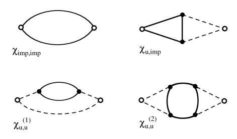
Figure 8: Feynman diagrams for the susceptibility to a uniform magnetic field. The open circles are external sources, the filled circles represent the interaction which contributes a factor $K$, the full lines are propagators of the auxiliary fermions ${f}$ representing the impurity spin, and the dashed lines are ${t}$ propagators.

Note that there are two contributions to $\chi_{\text{u,u}}=2\chi_{\text{u,u}}^{(1)}+\chi_{\text{u,u}}^{(2)}$ where $\chi_{\text{u,u}}^{(2)}$ has four interaction vertices. At the critical point ($s=s_{c}$) the four diagrams have the following low-temperature behavior:

$$\chi_{\text{u,u}}^{(1)}\sim{1\over T}\> \quad\chi_{\text{u,u}}^{(2)}\sim{1\over T}$$ , (159)

$$\chi_{\text{imp,imp}}\sim{{{\tilde{K}}}^{-\epsilon}\over T^{1-\epsilon}}\> \quad\chi_{\text{imp,u}}\sim{{{\tilde{K}}}^{-\epsilon/2}\over T^{1-\epsilon/2}}\>.$$ ,

In the gapped phase at low temperatures, $T\ll\Delta\ll{\tilde{K}}$, the susceptibilities are

$$\chi_{\text{u,u}}^{(1)}\sim{1\over\Delta}\> \quad\chi_{\text{u,u}}^{(2)}\sim{1\over T}\,,$$ , (160)

$$\chi_{\text{imp,imp}}\sim\left({\Delta\over{\tilde{K}}}\right)^{\epsilon}\frac{1}{T}\> \quad\chi_{\text{imp,u}}\sim\left({\Delta\over{\tilde{K}}}\right)^{\epsilon/2}\frac{1}{T}\>.$$ ,

We now proceed by combining the results into observable quantities. First, we have the impurity susceptibility, $\chi_{\text{imp}}$, as defined in (11). It is given by

$$\chi_{\text{imp}}=\chi_{\text{imp,imp}}+2\chi_{\text{imp,u}}+\chi_{\text{u,u}}\,.$$ (161)

From (159), (160) and $m,\Delta\ll{\tilde{K}}$ in the scaling limit it follows that the low-temperature behavior of $\chi_{\text{imp}}$ is dominated by $\chi_{\text{u,u}}$, whereas the other contributions can be considered as corrections to scaling. The impurity susceptibility takes the scaling form quoted in (76), with the universal scaling function $\Phi_{\text{imp}}$ given by

$$\Phi_{\text{imp}}\left(\frac{\Delta}{T}\right)=2\Phi_{\text{u,u}}^{(1)}\left(\frac{\Delta}{T}\right)+\Phi_{\text{u,u}}^{(2)}\left(\frac{\Delta}{T}\right)\,,$$

$$\chi_{\text{u,u}}^{(1)}=\frac{1}{T}\Phi_{\text{u,u}}^{(1)}\left(\frac{\Delta}{T}\right),\>\chi_{\text{u,u}}^{(2)}=\frac{1}{T}\Phi_{\text{u,u}}^{(2)}\left(\frac{\Delta}{T}\right)$$ (162)

Consistent with our predictions, there are no anomalous dimensions involved in $\chi_{\text{imp}}$, the reduced coupling constant ${\tilde{K}}$ and the bulk energy scale ${J}$ have dropped out. The contributions to the susceptibility can be evaluated numerically. At the critical coupling, $s=s_{c}$, we find $\chi_{\text{imp}}$ to have a Curie form, $\chi_{\text{imp}}=\mathcal{C}_{1}/k_{B}T$, as predicted in the introduction (31), with a universal prefactor $\mathcal{C}_{1}$ defining an effective spin, as discussed in the caption to Fig 3. In $d=2$, the large $N$ value of $\mathcal{C}_{1}$ is

$$\mathcal{C}_{1}=\mathcal{C}_{\text{free}}[0.59\pm 0.01],\,,$$ (163)

where $\mathcal{C}_{\text{free}}$ is defined in (158).

In the gapped phase at $T\ll\Delta$, it is seen from (160) that the low-$T$ behavior of $\chi_{\text{imp}}$ is determined by $\chi_{\text{u,u}}^{(2)}$ alone. As shown in Appendix E, the Curie prefactor of $\chi_{\text{u,u}}^{(2)}$ equals that of a free spin, i.e., $\Phi_{\text{u,u}}^{(2)}(\Delta/T\rightarrow\infty)=1/8$. This implies that in the gapped phase the impurity contributes to the total uniform susceptibility in the same manner as a free spin, i.e., we have shown the confinement of the impurity spin.

As a second observable, we again consider the local susceptibility which is defined as the response of the system to a magnetic field applied to the impurity spin only. It is given by $\chi_{\text{loc}}=\chi_{\text{imp,imp}}$, and is proportional to the autocorrelation function of the of the impurity spin at zero frequency. In the large-$N$ limit it is simply given by

$$\chi_{\text{loc}}=-\int_{0}^{\beta}{\rm d}\tau\>G_{f}(\tau)G_{f}(-\tau)\>.$$ (164)

If we evaluate this integral using the scaling solution for $G_{f}$ we arrive at

$$\chi_{\text{loc}}={{{\tilde{K}}}^{-\epsilon}\over T^{1-\epsilon}}\>\Phi_{\text{loc}}\left(\frac{\Delta}{T}\right)$$ (165)

with the universal scaling function $\Phi_{\text{loc}}(\Delta/T)$ determined by $\Phi_{G}(\tau T,\Delta/T)$ from Eq. (148):

$$\Phi_{\text{loc}}\left(\frac{\Delta}{T}\right)=\int_{0}^{1}{\rm d}\tilde{\tau}\>\Phi_{G}^{2}\left(\tilde{\tau},\frac{\Delta}{T}\right)\>.$$ (166)

The asymptotic behavior of $\Phi_{\text{loc}}(\Delta/T)$ is found to be

$$\Phi_{\text{loc}}(\tilde{\Delta})\sim\left\{\begin{array}[]{l}{\rm const}\>\>\>\>{\tilde{\Delta}}\ll 1\\ {\tilde{\Delta}}^{\epsilon}\>\>\>\>\,\quad{\tilde{\Delta}}\gg 1\end{array}\right.\>.$$ (167)

The local impurity susceptibility diverges at $s=s_{c}$ as $T^{-1+\epsilon}$, similarly the impurity spin autocorrelation function decays as $\tau^{-\epsilon}$ at the critical coupling. This implies that we have $\eta^{\prime}=\epsilon$ in the large-$N$ limit. For $T\ll\Delta$, $\chi_{\text{loc}}$ follows a Curie law with a prefactor of $(\Delta/{\tilde{K}})^{\epsilon}$ which corresponds to a remnant impurity moment of

$$m_{\text{imp}}\sim\left(\frac{\Delta}{{\tilde{K}}}\right)^{\epsilon/2}\sim|s-s_{c}|^{\eta^{\prime}\nu/2}\,,\quad\eta^{\prime}=\epsilon$$ (168)

consistent with the prediction (37).

IV Self-consistent NCA analysis: Finite impurity density

In this section we will discuss the case of a finite density of magnetic impurities using the formalism presented in Section III. A finite impurity density can lead to variety of phenomena which were discussed in Sections I.2 and I.3.2; we will restrict our attention here to the scattering of the bulk spin excitations from the impurities. Interactions between the impurities which eventually may lead to an ordered state at very low temperatures will be neglected. We shall assume $T\ll\Delta$ and work directly in $d=2$ and real frequency; all Green’s functions are retarded quantities, $\omega$ implicitly carries a positive imaginary part everywhere. All the computations in this section will be for the case in which all impurities have spin $S_{r}=1/2$.

The important new effect from a finite $n_{\text{imp}}$ is that bulk spin excitations described by the Green’s function $G_{t}$ acquire a self-energy from the scattering at the impurities—this changes the local density of states of the bulk excitations. We will determine the modified density of states self-consistently in this subsection.

The lowest-order scattering process for the ${t}$ bosons is described by the $T$-matrix $T_{t}(\omega)$ given by the bubble diagram of fermion Green’s functions:

$$T_{t}(\omega)={K}^{2}T\sum_{\omega_{n}}G_{{f}}(i\omega_{n})G_{{f}}(\omega-i\omega_{n})\>.$$ (169)

The interaction $\mathcal{H}_{\text{imp}}$ gives rise a momentum-dependent self-energy for the ${t}$ bosons. If we neglect higher-order scattering contributions (Born approximation) the self-energy is given by

$$\Sigma_{t}({\bf k},\omega)=n_{\rm imp}{2{J}A_{\bf k}\over{\epsilon}_{\bf k}}T_{t}(\omega)$$ (170)

where $n_{\rm imp}$ is the impurity concentration, and we have already performed an averaging over the (randomly distributed) impurities in the sample. The Green’s function $G_{tt}({\bf k},\omega)$ in the presence of scattering can be written as [cf. (139)]

$$G_{tt}({\bf k},\omega)={4{J}A_{\bf k}\over\omega^{2}-[{\epsilon}_{\bf k}+\Sigma_{t}({\bf k},\omega)]^{2}}\,.$$ (171)

In the scaling limit we can replace $A_{\bf k}$ by $A_{0}$ as above leading to

$$G_{tt}(k,\omega) = {4{J}A_{0}\over\omega^{2}-{\epsilon}_{k}^{2}-\Sigma_{tt}(\omega)}\>.$$ (172)

where the self-energy $\Sigma_{tt}$ ($\ll\!{\epsilon}_{k})$ is now momentum-independent, it is given by

$$\Sigma_{tt}(\omega)=2{\epsilon}_{k}\Sigma_{t}(k,\omega)=4n_{\text{imp}}{J}A_{0}T_{t}(\omega)\,.$$ (173)

The momentum integral can be performed in the scaling limit

$$G_{tt,\rm loc}(\omega) = \frac{2{J}A_{0}S_{2}}{c^{2}}\>\ln(m^{2}+\Sigma_{tt}(\omega)-\omega^{2})$$ (174)

which replaces the expression (142) found at zero impurity concentration. We have used ${\epsilon}_{k}^{2}=c^{2}k^{2}+m^{2}$. It is important to note that the effective mass $m$ acquires a renormalization from the scattering processes since the Hartree contribution to $m$ contains a boson propagator which is affected by the impurities; $m$ has to be determined by book

$$\int\frac{d\omega}{2\pi}\frac{d^{d}k}{(2\pi)^{d}}\left(G_{tt}(k,\omega)-G_{tt}^{(0)}(k,\omega)\right)=0$$ (175)

where $G_{tt}^{(0)}$ denotes the Green’s function (142) in the absence of impurities. Equations (169), (173), (174) determine $G_{tt}$ from $G_{f}$, on the other hand $G_{f}$ is connected with $G_{tt}$ through the NCA equations (136), (137). Solutions have to be found self-consistently, this procedure is similar to a self-consistent Born approximation.

It is possible to write the solutions in terms of scaling functions, where the only additional parameter introduced by the impurities is the energy scale $\Gamma$ (24) defined in Section I. We restrict the presentation to zero temperature, and introduce scaling functions as follows:

$$G_{tt,\rm loc}(\omega) = \frac{2{J}A_{0}S_{2}}{c^{2}}\>\Phi_{tt}^{\prime}\left(\frac{\omega}{\Delta},\frac{\Gamma}{\Delta}\right)\,,$$

$$G_{f}(\omega) = (\Delta{\tilde{K}})^{-1/2}\>\>\Phi_{G}^{\prime}\left(\frac{\omega}{\Delta},\frac{\Gamma}{\Delta}\right)\,,$$

$$\Sigma_{tt}(\omega) = \Delta^{2}\>\Phi_{\Sigma}^{\prime}\left(\frac{\omega}{\Delta},\frac{\Gamma}{\Delta}\right)\,.$$ (176)

With the notations $\bar{m}=m/\Delta$, $\bar{\omega}=\omega/\Delta$, and $\bar{\Gamma}=\Gamma/\Delta$ we can re-write the equations (169), (173), (174):

$$\Phi_{tt}^{\prime}(\bar{\omega},\bar{\Gamma}) = \ln\left[\bar{m}+\Phi_{\Sigma}^{\prime}(\bar{\omega},\bar{\Gamma})-\bar{\omega}^{2}\right]\,,$$ (177)

$${\rm Im}\>\Phi_{\Sigma}^{\prime}(\bar{\omega},\bar{\Gamma}) = \frac{2\bar{\Gamma}}{S_{2}}\int\frac{d\bar{\omega}_{1}}{\pi}{\rm Im}\>\Phi_{G}^{\prime}(\bar{\omega}-\bar{\omega}_{1},\bar{\Gamma})$$

$$\times\>{\rm Im}\> \Phi_{G}^{\prime} (\bar{\omega}_{1},\bar{\Gamma})\left[n_{F}(\bar{\omega}_{1})-n_{F}(\bar{\omega}-\bar{\omega}_{1})\right]\,,$$

and the NCA equations (136), (137):

$${\rm Im}\left(\Phi_{G}^{\prime}(\bar{\omega},\bar{\Gamma})^{-1}\right) = \int\frac{d\bar{\omega}_{1}}{\pi}{\rm Im}\>\Phi_{G}^{\prime}(\bar{\omega}-\bar{\omega}_{1},\bar{\Gamma})$$ (178)

$$\times\>{\rm Im}\> \Phi_{tt}^{\prime} (\bar{\omega}_{1},\bar{\Gamma})\left[n_{B}(\bar{\omega}_{1})+n_{F}(\bar{\omega}-\bar{\omega}_{1})\right]\,.$$

The functions $n_{F}$ and $n_{B}$ are Fermi and Bose functions in the zero-temperature limit, $n_{F}(x)=\Theta(-x)$, $n_{B}(x)=-\Theta(-x)$, where $\Theta(x)$ is the step function. $\Phi_{G}^{\prime}$ and $\Phi_{\Sigma}^{\prime}$ are analytic functions of $\bar{\omega}$ in the upper-half complex plane, so their real parts are given by Kramers-Kronig relations. Finally, the renormalized mass $\bar{m}$ is determined by the constraint equation (175) written in terms of $\Phi_{tt}^{\prime}$. The system of equations (177), (178) can be solved self-consistently for a given value of $\Gamma/\Delta$, and universally describes the spin dynamics of both the host antiferromagnet and the impurities. For $\Gamma=0$ the equations of course reduce to the zero-temperature limit of the NCA equations (136), (137) quoted in Section III.

We now turn to the broadening of the boson spin-1 collective mode peak seen e.g. in a neutron scattering experiment. Therefore we have to calculate the dynamic spin susceptibility which is identical to the Green’s function $G_{tt}({\bf k},\omega)$. We consider the dynamic susceptibility at the antiferromagnet wavevector

$$\chi_{{\bf Q}}(\omega)=\frac{\mathcal{A}}{\Delta^{2}-\omega^{2}+\Sigma_{tt}(\omega)}\>.$$ (179)

The scaling form for $\Sigma_{tt}$ in (176) implies that $\chi_{{\bf Q}}(\omega)$ indeed obeys the scaling form (42) with the scaling function $\Phi$ given by

$$\Phi(\bar{\omega},\bar{\Gamma})^{-1}=1-(\bar{\omega}+i0^{+})^{2}+\Phi_{\Sigma}^{\prime}(\bar{\omega},\bar{\Gamma})$$ (180)

The results show that $\text{Im}\Phi(\bar{\omega})$ has a hard gap at small frequencies, with a gap size of $\sim 1-1.6\bar{\Gamma}$. The lineshape is strongly asymmetric with a tail at high frequencies. The half-width of the resulting line is approximately given by $\Gamma$, see Figs. 4 and 9.

Figure 9: Lineshapes $\text{Im}\Phi$ as a function of $\hbar\omega/\Delta$ similar to Fig. 4, but for $\Gamma/\Delta=0.05$, 0.1, 0.15, and 0.2.

The asymmetry of the line is a consequence of the interplay between the gap, $\Delta$, in the bulk antiferromagnet and the inelastic scattering from the impurity spin. The bulk magnons self-consistently form an ‘impurity band’ whose lower edge extends to an energy of order $\Gamma$ below $\Delta$. There is no phase space for scattering below this band edge, while frequencies above have scattering states readily available—the result is an asymmetric line.

We now apply the present analysis to the broadening of the ‘resonance peak’ observed recently in ${\rm Zn}$-doped ${\rm YBa}_{2}{\rm Cu}_{3}{\rm O}_{7}$ keimer . Using the values $\hbar c=0.2$ eV, $\Delta=40$ meV, and $n_{\rm imp}=0.005$, we obtain $\Gamma=5$ meV and $\Gamma/\Delta=0.125$. A linewidth of roughly 5 meV is in excellent accord with the measured value of 4.25 meV keimer . The lineshape observed in Ref. keimer, appears to be asymmetric in accordance with our analysis; however, future experiments should be able to test this prediction in more detail.

V Conclusions

The object of attention in this paper has been a ‘nearly-critical’, two-dimensional, host antiferromagnet with a spin-gap $\Delta$. We described this antiferromagnet by a universal, continuum, quantum field theory, $\mathcal{S}_{b}$: this is obtained obtained by deforming a O(3)-symmetric, 2+1 dimensional, conformally-invariant fixed point by its single relevant operator–the ‘mass’ term, $\phi_{\alpha}^{2}$, in (4). Then we ‘punctured’ this continuum field theory by quantum impurities at a collection of spatial point $\{r\}$. We argued that each such impurity was completely characterized by a single integer/half-odd-integer valued spin, $S_{r}$, which determined the Berry phase of spin precession, see (13). In particular, for a non-extensive number of impurities, there were no new relevant operators, and so the energy scale, $\Delta$, continued to characterize the dynamics of the antiferromagnet in the vicinity of the impurities. A non-zero density of impurities, $n_{\text{imp}}$, is a relevant perturbation, but its impact was universally determined entirely by the dimensionless number $\Gamma/\Delta=n_{\text{imp}}(\hbar c/\Delta)^{2}$, and was independent of the magnitude of the bare exchange between the impurities and the antiferromagnet. Results for many physical properties of this antiferromagnet were obtained.

We also showed how the above results could be extended to apply to d-wave superconductors. For the case where momentum conservation prohibits a coupling of bosonic $\phi_{\alpha}$ field to low energy fermionic Bogoliubov quasiparticles, no changes are necessary: the theory for the insulating antiferromagnet applies quantitatively to the collective spin excitations of the superconductor. The situation where there is an efficient coupling of $\phi_{\alpha}$ to the Bogoliubov quasiparticles is considered in Appendix A: we show there that the structure of all the scaling forms remains unchanged, but there are quantitative changes to the numerical values of the scaling functions.

As a guide to the reader who read Section I and skipped the body of the paper, we itemize our main results. For the case of a single impurity, our main results were as follows.

• The response to a uniform magnetic field is summarized in Fig 3. The $\epsilon$ expansion for the constant $\mathcal{C}_{1}$ is in (77): it is evident that the series cannot be used directly for a quantitative estimate, and we have not attempted any resummation analysis. The large-$N$ prediction for $\mathcal{C}_{1}$ is in (163) with $\mathcal{C}_{\text{free}}=1/4$. On the ordered side, the $\epsilon$ expansion for the constant $\mathcal{C}_{3}$ is in (125).

• Local response functions are governed by the known bulk anomalous dimension, $\eta$, and the new boundary anomalous dimension $\eta^{\prime}$. The $\epsilon$ expansion for the latter is in (68).

• The local susceptibility, $\chi_{\text{loc}}$, measures the impurity site response to a field applied at the impurity site only. The $\epsilon$ expansion for this is in (80,81), while the large-$N$ result is in (165).

• The Knight shift measures the localized response to a uniform magnetic field applied everywhere. The Knight shift very close to the impurity site is in (84,85). Away from the impurity site, there is a response which oscillates with the orientation of the Néel order parameter, as in Fig. 1— the envelope of this oscillating component is given in (89,91). There is also a smaller uniform (ferromagnetic) component to the Knight shift—this is in (98,99).

• In the ordered Néel state, the spontaneous moment on the impurity site obeys (37,114). Away from the impurity site, there is a staggered component obeying (117), and a uniform component obeying (119).

For the system with a finite density of impurities, we obtained results for the magnon lineshape in the spin gap phase. This line obeys the exact scaling form (42), and NCA results for the scaling function are in Figs 4 and 9, and in (177,178,180).

The rest of this section discusses some remaining experimental issues.

One interesting observation of the neutron scattering experiments of Ref keimer, was that Zn doping caused the resonance peak to appear at larger temperatures significantly above the superconducting transition temperature. We do not have a theory of the superconducting order in this paper, and so cannot directly address this question. However, this experimental result supports the interpretation that the resonance is very much like the gapped, spin-1 excitation in the paramagnetic phase of an antiferromagnet keimer ; lt . In the “swiss-cheese” model of Zn doping developed by Uemura and collaborators tomo , such antiferromagnetic correlations are enhanced in the vicinity of the impurity (as in Fig 1 and Refs. alloul2, ; alloul2a, ; julien, ), and should lead to increased stability of the resonance mode at higher temperatures.

Recent measurements of the effective moment on the Zn site in ${\rm YBa}_{2}{\rm Cu}_{3}{\rm O}_{6.7}$ at fairly large temperatures yield a value $p_{\text{eff}}\approx 1.0$ which is smaller than the value expected for $g=2$, $S=1/2$, $p_{\text{eff}}=g\sqrt{S(S+1)}=1.73$. While some of this reduction is surely due to inter-impurity interactions, we speculate that the crossover to the quantum-critical region is playing a role. In the latter regime, we expect $p_{\text{eff}}=g\sqrt{3\mathcal{C}_{1}}$; using the value in (163) we obtain $p_{\text{eff}}\approx 1.33$.

Next, we discuss the relationship of our work to analyses of impurity effects in d-wave superconductors lee ; sasha1 ; sasha2 ; kallin ; fradkin ; nl ; sigrist2 ; ogata ; fulde ; pepin and a recent tunneling experimentseamus . The former have all been carried out using actions closely related to $\mathcal{S}_{\Psi}+\mathcal{S}_{\Psi\text{imp}}$ (in (26,28). However, we have argued in this paper that the coupling of the impurity spin to the collective, spin-1, mode $\phi_{\alpha}$ is a more relevant perturbation. One consequence of such a coupling is that the impurity spin has structure in its spectral function at frequencies which are integer multiples of $\Delta$, as we found in Section III.3.2. It is therefore natural to expect that some of this structure will appear also in the quasiparticle tunneling spectrum: it is interesting that a sideband at a frequency of order $\Delta$ does appear to be present in the tunneling spectrum at the impurity site in Ref. seamus, . As we move away from the impurity site, the coupling between the quasiparticles and the $\phi_{\alpha}$ mode becomes negligible, and the frequency $\Delta$ should not be visible in tunneling—this also appears to be consistent with Ref. seamus, . We note that this sideband phenomenon is similar in spirit to arguments made by Abanov and Chubukov chubukov for photoemission experiments photo . Also, some related computations on the relationship of tunneling spectra to antiferromagnetic collective modes appear in a recent work by Chubukov et al. nathan

In closing, we mention some consequences of our theory to Ni doping of two-dimensional spin-gap compounds of spin-1/2 Cu ions. Each Ni ion has spin-1, and so the net uncompensated moment in its vicinity will still have $S_{r}=1/2$. Our theory, therefore implies that the damping of the bulk $\phi_{\alpha}$ quasiparticle mode due to the Ni impurities will be the same as that due to non-magnetic Zn impurities, because both depend only the bulk parameters and the values of $S_{r}$; all differences arise only from irrelevant couplings and these are suppressed by factors of $\Delta/J$. However, the atomic scale, staggered spin polarization will be very different in the two cases; in particular, a large contribution to the net moment of $S_{r}=1/2$ comes from the magnetic moment on the Ni ion itself, while no magnetic moment is present on the Zn ions: this implies strong differences in the STM spectra.

Appendix A Fermionic quasiparticles in d-wave superconductors

This appendix will continue the discussion of Section I.2.1 on the consequences of the gapless, fermionic, Bogoliubov excitations in a d-wave superconductor. As was noted in Section I.2.1, for quasiparticles with vanishing energy at wavevectors $(\pm K,\pm K)$, the key issue was whether the antiferromagnetic wavevector, ${\bf Q}$, equaled $(2K,2K)$ or not. For ${\bf Q}\neq(2K,2K)$, the bulk coupling between the antiferromagnetic order parameter, $\phi_{\alpha}$ and the fermionic quasiparticles can be neglected at low enough energies, and this was assumed in the body of the paper. In this appendix, we describe the changes necessary for ${\bf Q}=(2K,2K)$.

A.1 Host superconductor

The critical theory of an antiferromagnetic ordering transition in a d-wave superconductor with ${\bf Q}=(2K,2K)$ was described recently by Balents, Fisher and Nayak balents . Here we will review their results in a field-theoretic approach designed for efficient treatment of the impurity problem.

First, we specify the fermionic action (26) more precisely. Let the components of electron annihilation operator in the vicinity of the wavevectors $(K,K)$, $(-K,K)$, $(-K,-K)$, $(K,-K)$ be $f_{1a}$, $f_{2a}$, $f_{3a}$, $f_{4a}$ respectively, where $a=\uparrow,\downarrow$ is the electron spin component. Now introduce the 4-component Nambu spinons $\Psi_{1}=(f_{1a},\varepsilon_{ab}f_{3b}^{\dagger})$ and $\Psi_{2}=(f_{2a},\varepsilon_{ab}f_{4b}^{\dagger})$ where $\varepsilon_{ab}$ is an antisymmetric tensor with $\varepsilon_{\uparrow\downarrow}=1$. Then the full form of (26) is

$$\mathcal{S}_{\Psi} = \int\frac{d^{d}k}{(2\pi)^{d}}T\sum_{\omega_{n}}\Psi_{1}^{\dagger}\left(-i\omega_{n}+k_{x}\tau^{z}+k_{y}\tau^{x}\right)\Psi_{1}$$ (181)

$$\!\!\!\!\!\!\!\!\!\!\!\!\!\!+\int\frac{d^{d}k}{(2\pi)^{d}}T\sum_{\omega_{n}}\Psi_{2}^{\dagger}\left(-i\omega_{n}+k_{y}\tau^{z}+k_{x}\tau^{x}\right)\Psi_{2}.$$

Here $\tau^{\alpha}$ are Pauli matrices which act in the fermionic particle-hole space, the wavevectors $k_{x,y}$ have been rotated by 45 degrees from the axes of the square lattice, and we have scaled the fermionic velocities to unity (following Ref. balents, , we assume that the velocities in the two directions are equal near the critical point). With ${\bf Q}=(2K,2K)$, the allowed bulk coupling between the antiferromagnetic order parameter $\phi_{\alpha}$ and $\Psi_{1,2}$ is balents

$${\cal S}_{\Psi\phi}=\int d^{2}xd\tau\left(\frac{\lambda_{0}}{2}\phi_{\alpha}\Psi_{1}\sigma^{y}\sigma^{\alpha}\tau^{y}\Psi_{1}+\mbox{H.c.}+(1\rightarrow 2)\right),$$ (182)

where $\sigma^{\alpha}$ are Pauli matrices in spin space.

The antiferromagnetic ordering transition in the d-wave superconductor is described by the action $\mathcal{S}_{b}+\mathcal{S}_{\Psi}+\mathcal{S}_{\Psi\phi}$ specified in (4), (181), (182). We perform its renormalization group analysis in $d=3-\epsilon$ dimensions by the renormalizations (52) and

$$\Psi_{1,2} = Z_{f}^{1/2}\Psi_{1,2R}$$

$$\lambda_{0} = \frac{\mu^{\epsilon/2}}{S_{d+1}^{1/2}}\frac{Z_{\lambda}}{Z_{f}Z^{1/2}}\lambda.$$ (183)

At one loop, the results of Ref balents, translate to the following renormalization constants in the minimal subtraction scheme ((54) no longer applies):

$$Z = 1-\frac{4\lambda^{2}}{\epsilon}-\frac{5g^{2}}{144\epsilon}$$

$$Z_{4} = 1+\frac{11g}{6\epsilon}-\frac{48\lambda^{4}}{g\epsilon}$$

$$Z_{f} = 1-\frac{3\lambda^{2}}{2\epsilon}$$

$$Z_{\lambda} = 1-\frac{\lambda^{2}}{\epsilon}.$$ (184)

We have taken the liberty of adding a single additional two-loop contribution above: the order $g^{2}$ term for $Z$ which was also present in (54). These translate into the beta functions (replacing (62))

$$\beta(g) = -\epsilon g+\frac{11g^{2}}{6}+8\lambda^{2}g-48\lambda^{4}$$

$$\beta(\lambda) = -\frac{\epsilon\lambda}{2}+\frac{5\lambda^{3}}{2}.$$ (185)

The stable fixed point of these equations is

$$g^{\ast} = \frac{48\epsilon}{55}$$

$$\lambda^{\ast 2} = \frac{\epsilon}{5},$$ (186)

and the value of $g^{\ast}$ replaces that in (66). The anomalous dimension in (67) is replaced by

$$\eta = \frac{4\epsilon}{5}+\ldots$$

$$\eta_{f} = \frac{3\epsilon}{10}+\ldots,$$ (187)

where $\eta_{f}$ is anomalous dimension of the fermions $\Psi_{1,2}$.

These fixed point couplings can be used to compute the universal correlations of the antiferromagnetic order parameter. In particular, in the paramagnetic phase, the dynamic susceptibility at the antiferromagnetic wavevector obeys (41), where $\Delta$ is an energy scale measuring the distance from the critical point to long-range antiferromagnetic order. To leading order in $\epsilon$ we find

$$\chi_{\bf Q}(\omega)=\frac{1}{\Delta^{2}-\omega^{2}-\Sigma_{\bf Q}(\omega)},$$ (188)

with a self-energy, $\Sigma_{\bf Q}$, with imaginary part

$$\mbox{Im}\Sigma_{\bf Q}(\omega=\Delta)=\epsilon\frac{2\pi\Delta^{2}}{5}.$$ (189)

This is the main difference between the antiferromagnetic transition in an insulator and a d-wave superconductor with ${\bf Q}=(2K,2K)$: the scaling structure in the two cases is identical, but the latter has damping in the $\phi_{\alpha}$ collective mode of the paramagnetic phase even at $T=0$.

A.2 Quantum impurities

As discussed in Section I.2, we couple quantum impurities to the bulk theory of Appendix A.1. The fermionic couplings in $\mathcal{S}_{\Psi\text{imp}}$ (Eqn. (28)) continue to be irrelevant, and so we discuss the theory with action $\mathcal{S}_{b}+\mathcal{S}_{\text{imp}}+\mathcal{S}_{\Psi}+\mathcal{S}_{\Psi\phi}$ specified in (4), (13), (181), (182).

The analysis is essentially identical to that in Section II.1. At the one loop level, there are no new Feynman diagrams, and only those in Fig 5 appear. Moving to the two loop level, we find the diagrams in Fig 6, 11, 12, and also the single new category of diagrams in Fig 10.

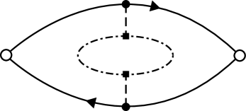
Figure 10: Additional contribution to the correlator of Fig 5 in the theory of Appendix A. Each propagator of $\phi_{\alpha}$ (represented by the dashed line) in Fig 5 acquires a fermion loop (represented by the dash-dot line) self energy correction; the filled square is the $\lambda_{0}$ coupling. Only the correction to one diagram of Fig 5 is shown here; corresponding corrections to the others are implied.

Evaluating these new diagrams, we find that at this order, the value of the boundary renormalization constant $Z_{\gamma}$ remains unchanged to that in (60), while the constant $Z^{\prime}$ is modified from (61) to

$$Z^{\prime}=1-\frac{2\gamma^{2}}{\epsilon}+\frac{\gamma^{4}}{\epsilon}+2\gamma^{2}\lambda^{2}\left(-\frac{2}{\epsilon^{2}}+\frac{1+2C-\ln 4}{\epsilon}\right),$$ (190)

where $C=0.5772\ldots$ is Euler’s constant. The renormalization constants in (60,184,190) modify the beta function for the boundary coupling $\gamma$ from (65) to

$$\beta(\gamma) = -\frac{\epsilon\gamma}{2}+\gamma^{3}+2\lambda^{2}\gamma-\gamma^{5}+\frac{5g^{2}\gamma}{144}$$ (191)

$$+\frac{g\gamma^{3}\pi^{2}}{3}[S(S+1)-1/3]-2\lambda^{2}\gamma^{3}(1+2C-\ln 4)$$

$$+\vartheta\lambda^{4}\gamma.$$

Here $\vartheta$ is a numerical coefficient whose determination requires the order $\lambda^{4}$ term in the bulk renormalization factor $Z$ in (184); the latter has not yet been computed. Eqn (191) modifies the fixed point value $\gamma^{\ast}$ from (66) to

$$\gamma^{\ast 2}=\frac{\epsilon}{10}+\ldots$$ (192)

Armed with the fixed point values in (186,192), we can now extend all the computations of Section II to the theory of this appendix. There are no changes in the structure of the exact scaling forms, but the scaling functions and exponents have to be recomputed in the present theory. In particular, the value of the boundary anomalous dimension $\eta^{\prime}$ changes from (68) to

$$\eta^{\prime}=\frac{\epsilon}{5}+\ldots.$$ (193)

Appendix B Incommensurate spin correlations

The body of the paper considered antiferromagnets with a collinear spin polarization commensurate with the underlying lattice. Here we discuss the case of incommensurate spin correlations.

Several classes of incommensurate magnets need to be distinguished. If the incommensurate order is spiral, then the spin polarization is non-collinear, and a very different theory is necessary book –the quantum paramagnetic phases of such magnets possibly have deconfined excitations, and their coupling to the impurity spin will be quite different. We will not consider such a situation here.

Restricting attention to incommensurate collinear antiferromagnets, we have to further distinguish two cases. Let us describe the spin polarization in the ordered phase of such a magnet by

$$\langle\hat{S}_{\alpha}(x)\rangle=\text{Re}\left(N_{\alpha}e^{i{\bf Q}\cdot x}\right),$$ (194)

where ${\bf Q}$ is the incommensurate ordering wavevector, and $N_{\alpha}$ is a complex three-component field. Associated with any such spin polarization, simple symmetry considerations kivelson imply that there must be a corresponding charge density modulation

$$\langle\delta\rho(x)\rangle\propto\cos(2{\bf Q}\cdot x+\varphi),$$ (195)

where $\varphi$ is an arbitrary phase offset. The final situation depends upon the status of the charge density modulation at the quantum transition at which the magnetic order disappears. If the magnetic order (194) vanishes while the charge modulation in (195) is preserved on both sides of the transition, then the theory in the body of the paper continues to apply to the spin excitations. This is because we may view the spin modulation as (in a sense) commensurate with the underlying charge density wave—in other words, the value of $\varphi$ pins the phase of $N_{\alpha}$ and the order parameter becomes effectively real. Only in the case where the modulations in (194) and (195) vanish at the same quantum critical point is a new theory necessary (the remaining case, in which the order (195) vanishes, while (194) is preserved is not possible on general symmetry grounds). We have to extend the theory $\mathcal{S}_{\text{b}}+\mathcal{S}_{\text{imp}}$ from a real field $n_{\alpha}$ to a complex field $N_{\alpha}$. We will not enter into this in any detail, but mention the changes necessary. In $\mathcal{S}_{\text{b}}$, in addition to the usual quartic term, $(N^{\ast}_{\alpha}N_{\alpha})^{2}$, a second quartic term, $|N_{\alpha}N_{\alpha}|^{2}$ is permitted; in $\mathcal{S}_{\text{imp}}$, the coupling $\gamma_{0r}$ becomes complex. The phase of $\gamma_{0r}$ is a renormalization group invariant (rather than just its sign), and its initial value plays a role similar to that of $\sigma_{r}$.

Appendix C Diagrammatic perturbation theory

We describe a diagrammatic approach to expanding arbitrary correlators $\mathcal{S}_{\text{b}}+\mathcal{S}_{\text{imp}}$ in powers of $\gamma_{0}$ and $g_{0}$. We will restrict ourselves to a single impurity here, with the notations (30) and (43). The generalization to the many impurity case is straightforward.

The simplest way to generate this is to use a Hamiltonian representation of the quantum spin in terms of Heisenberg spin operators; so we replace

$$Sn_{\alpha}\rightarrow\hat{S}_{\alpha},$$ (196)

where the $\hat{S}_{\alpha}$ satisfy the standard spin commutation relations

$$[\hat{S}_{\alpha},\hat{S}_{\beta}]=i\epsilon_{\alpha\beta\gamma}\hat{S}_{\gamma}.$$ (197)

Now we represent the partition function as a time-ordered exponential of the interaction terms, expand the exponential in powers of $\gamma_{0}$ and $g_{0}$, and take the trace over the Hilbert space of the spin operators. Closely related methods have been developed for the traditional Kondo problem hewson .

We can reduce the results of such an expansion to a simple set of diagrammatic rules. It is important to remember that there is no automatic cancellation of disconnected diagrams in such an approach. So when evaluating the expectation value $\langle O\rangle$ of an arbitrary observable $O$,

$$\langle O\rangle=\frac{\text{Tr}(OZ)}{\text{Tr}Z},$$ (198)

we must separately expand the numerator and denominator consistently to each order in $\gamma_{0}$ and $g_{0}$. The diagrammatic rules can be applied to both these expansions.

We represent the time evolution of the spin operator by a single, directed loop along which imaginary time runs periodically from 0 to $\beta$. This loop is shown as a full line, and there is one, and only one, loop in each diagram. Each factor of $\gamma_{0}$ is associated with a filled circle on the loop at some time $\tau_{i}$. Associated with each such filled circle we have:

• A propagator for the $\phi_{\alpha}$ field emerges from the filled circle (represented by a dashed line), and these are contracted together in powers of $g_{0}$ by standard $\phi_{\alpha}^{4}$ perturbation theory. The $g_{0}$ interaction is represented by a wavy line.

• A factor of the spin operator $\hat{S}_{\alpha}$—these are placed in order of the increasing $\tau_{i}$ and then the trace is taken over the spin Hilbert space. There are also factors of $\hat{S}_{\alpha}$ associated with external sources of $Sn_{\alpha}$ in the operator $O$—these are represented by open circles.

• All the times $\tau_{i}$ are integrated over the maximum possible interval between $0$ to $\beta$ subject to the constraint that they maintain their time ordering along the directed loop.

All of the diagrams contributing at order $\gamma_{0}^{2}$ to the numerator and denominator of the two-point correlator of the $n_{\alpha}$ are shown in Fig 5. As an application of the rules above, we see that the contribution of the last diagram in the numerator (the one with the time labels shown) is

$$\gamma_{0}^{2}\text{Tr}\left(\hat{S}_{\alpha}\hat{S}_{\beta}\hat{S}_{\alpha}\hat{S}_{\beta}\right)\int_{0}^{\tau}d\tau_{1}\int_{\tau}^{\beta}d\tau_{2}D(\tau_{1}-\tau_{2}).$$ (199)

The trace over spin operators evaluates to

$$\text{Tr}\left(\hat{S}_{\alpha}\hat{S}_{\beta}\hat{S}_{\alpha}\hat{S}_{\beta}\right)=(2S+1)S(S+1)[S(S+1)-1]$$ (200)

Other diagrams can be evaluated similarly, and we obtain (45) after the quotient has been taken.

Proceeding to order $\gamma_{0}^{4}$ for the same correlator, the graphs shown in Fig 11 are added to the numerator,

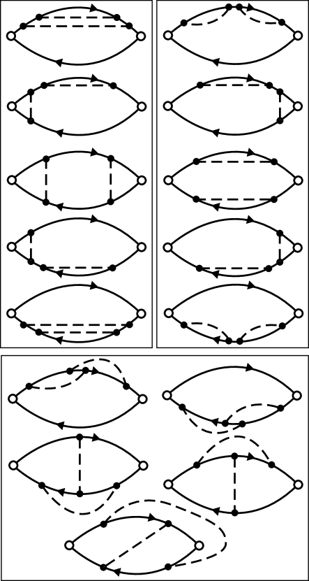
Figure 11: Contributions to the numerator of the correlator (45) at order $\gamma_{0}^{4}$. These have to be added to the diagrams in Fig 5a. They have been collected in groups of 5 for reasons described in Appendix C.

Figure 12: Contributions to the denominator of the correlator (45) at order $\gamma_{0}^{4}$. These have to be added to the diagrams in Fig 5b.

while those shown in Fig 12 add to the the denominator. The new non-trivial spin traces which arise are

$$\text{Tr}\left(\hat{S}_{\alpha}\hat{S}_{\beta}\hat{S}_{\gamma}\hat{S}_{\beta}\hat{S}_{\alpha}\hat{S}_{\gamma}\right)=(2S+1)$$

$$\qquad\times S(S+1)[S^{2}(S+1)^{2}-2S(S+1)+1]$$

$$\text{Tr}\left(\hat{S}_{\alpha}\hat{S}_{\beta}\hat{S}_{\gamma}\hat{S}_{\alpha}\hat{S}_{\beta}\hat{S}_{\gamma}\right)=(2S+1)$$

$$\qquad\times S(S+1)[S^{2}(S+1)^{2}-3S(S+1)+2].$$ (201)

We now take the quotient of the additional contributions from Fig 11 and 12. Although this can be a laborious process, the work can be shortened by observing many cancellations diagrammatically. We have collected the diagrams in Fig 11 in groups of 5 to aid this process; all the diagrams within each group differ only by a time displacement on the $\gamma_{0}$ interactions through the external vertices. Indeed, the union of the domains of the time integrals in each group precisely equals the domain of the time integral of a single diagram in Fig 12. Were it not for the differences between the traces of the spin operators in (201), these contributions to the numerator and the denominator would precisely cancel. Consequently, we need only keep track of such differences, and can then quickly write down the final quotient. The result is the following contribution to the two-point $n_{\alpha}$ correlator at order $\gamma_{0}^{4}$:

$$\gamma_{0}^{4}S(S+1)\int_{0}^{\tau}\!\!d\tau_{1}\int_{\tau}^{\beta}\!\!d\tau_{2}D(\tau_{1}-\tau_{2})\Bigg{[}$$

$$\quad\int_{0}^{\tau_{1}}\!\!d\tau_{3}\int_{\tau_{1}}^{\tau}\!\!d\tau_{4}+\int_{\tau}^{\tau_{2}}\!\!d\tau_{3}\int_{\tau_{2}}^{\beta}\!\!d\tau_{4}+2\int_{0}^{\tau_{1}}\!\!d\tau_{3}\int_{\tau}^{\tau_{2}}\!\!d\tau_{4}$$

$$\qquad\qquad+\int_{0}^{\tau_{1}}\!\!d\tau_{3}\int_{\tau_{2}}^{\beta}\!\!d\tau_{4}\Bigg{]}D(\tau_{3}-\tau_{4})$$ (202)

After carefully taking the $T=0$ limit of the above expression as described above (48), and evaluating the integrals using (49), we obtain the two-loop contribution in (51).

Appendix D Dynamic correlations in the paramagnet

At $T=0$, and $s\geq s_{c}$, the two-point correlations of the renormalized $n_{R\alpha}$ field can be written down from (45):

$$S^{2}\langle n_{R\alpha}(\tau)n_{R\alpha}(0)\rangle=S(S+1)\bigg{[}1$$

$$\qquad\qquad-2\gamma^{2}\int_{0}^{\tau}d\tau_{1}\int_{-\infty}^{0}d\tau_{2}D(\tau_{1}-\tau_{2})\bigg{]}/Z^{\prime},$$ (203)

where have retained terms accurate only to order $\gamma^{2}$, and at $T=0$, $D(\tau)$ in (46) evaluates to

$$D(\tau)=\frac{2^{(3-d)/2}\Delta^{d-1}}{\Gamma((d-1)/2)}\frac{\widetilde{S}_{d+1}}{(\Delta\tau)^{(d-1)/2}}K_{(d-1)/2}(\Delta\tau),$$ (204)

with $K_{(d-1)/2}(\Delta\tau)$ a modified Bessel function. The $\Delta=0$ limit of (204) is (49).

We first evaluate (203) at the critical point $\Delta=0$. Performing the integral and using (61) we have

$$S^{2}\langle n_{R\alpha}(\tau)\cdot n_{R\alpha}(0)\rangle=S(S+1)\left(1-2\gamma^{2}[1+\ln(\mu\tau)]\right)$$ (205)

to leading order in $\epsilon$- the poles in $\epsilon$ have cancelled. For large $\tau$ we can exponentiate this at the fixed point coupling value $\gamma^{*2}=\epsilon/2$ and find that

$$S^{2}\langle n_{R\alpha}(\tau)\cdot n_{R\alpha}(0)\rangle=S(S+1)\frac{1}{(\mu\tau)^{\epsilon}}$$ (206)

which predicts $\eta^{\prime}=\epsilon$ to leading order in $\epsilon$.

We now consider the $\tau\rightarrow\infty$ limit of the correlations for $\Delta>0$:

$$\lim_{\tau\rightarrow\infty}S^{2}\langle n_{\alpha}(\tau)\cdot n_{\alpha}(0)\rangle=S(S+1)\bigg{[}1$$

$$\qquad\qquad-2\gamma_{0}^{2}\int_{0}^{\infty}d\tau_{1}\int_{-\infty}^{0}d\tau_{2}D(\tau_{1}-\tau_{2})\bigg{]}$$ (207)

Introducing new dimensionless coordinates $y=\Delta(\tau_{1}-\tau_{2}),\,x=\Delta(\tau_{1}+\tau_{2}$), we write

$$\lim_{\tau\rightarrow\infty}S^{2}\langle n_{\alpha}(\tau)\cdot n_{\alpha}(0)\rangle=S(S+1)\bigg{[}1$$

$$\qquad\qquad-\frac{2\gamma_{0}^{2}}{\Delta^{2}}\int_{0}^{\infty}dyyD(y/\Delta)\bigg{]}$$ (208)

The relevant integral to be evaluated is (with $\alpha=(d-1)/2$)

$$\int_{0}^{\infty}dyy\cdot y^{-\alpha}K_{\alpha}(y)$$

$$\quad=\int_{0}^{1}dyy^{1-\alpha}K_{\alpha}(y)+\int_{1}^{\infty}dyy^{1-\alpha}K_{\alpha}(y)$$

$$\quad\approx\int_{0}^{1}\!\!dyy^{1-\alpha}\frac{\Gamma(\alpha)}{2}\left(\frac{y}{2}\right)^{-\alpha}+\int_{1}^{\infty}\!\!dyy^{1-\alpha}\left(\frac{\pi}{2y}\right)^{1/2}e^{-y}$$

$$\quad=\frac{2^{\alpha-1}\Gamma(\alpha)}{2-2\alpha}+\left(\frac{\pi}{2}\right)^{1/2}\Gamma(3/2-\alpha,1)$$ (209)

In the second line above we have used the asymptotic forms of the function $K_{\alpha}(y)$ for very small and large values of its argument abramowitz , and $\Gamma(3/2-\alpha,1)$ is the incomplete Gamma function. Now putting it all back together

$$\lim_{\tau\rightarrow\infty}S^{2}\langle n_{\alpha}(\tau)\cdot n_{\alpha}(0)\rangle=S(S+1)\bigg{[}1$$

$$\qquad-2\gamma^{2}\left(\frac{1}{\epsilon}\left(\frac{\mu}{\Delta}\right)^{\epsilon}+\left(\frac{\pi}{2}\right)^{1/2}\Gamma(1/2,1)\right)\bigg{]}$$ (210)

Recalling the definition of $Z^{\prime}$ (61), we conclude that

$$\lim_{\tau\rightarrow\infty}S^{2}\langle n_{R\alpha}(\tau)\cdot n_{R\alpha}(0)\rangle=S(S+1)\bigg{[}1$$

$$\qquad-2\gamma^{2}\left(\ln\frac{\mu}{\Delta}+\left(\frac{\pi}{2}\right)^{1/2}\Gamma(1/2,1)\right)\bigg{]}$$ (211)

Near the fixed point we use $\gamma^{*2}=\epsilon/2$ and exponentiate to obtain from (36) that $m_{\text{imp}}\sim(\Delta/\mu)^{\epsilon/2}$, which agrees with (37) and $\eta^{\prime}=\epsilon$.

Appendix E Details of the large-$N$ calculation

This appendix provides some details of the large-$N$ calculations presented in Section III.

First we prove that the chemical potential ${\lambda_{0}}=0$ in the particle-hole symmetric case $q_{0}=\frac{1}{2}$. From $G_{tt}(\tau)=G_{tt}(\tau)^{*}=G_{tt}(-\tau)$ and $G_{f}(\tau)=G_{f}(\beta-\tau)=-G_{f}(-\tau)$ (for $q_{0}=\frac{1}{2}$) follows that $G_{f}(i\omega_{n})$ is purely imaginary, $G_{f}(i\omega_{n})=-G_{f}(i\omega_{n})^{*}=-G_{f}(-i\omega_{n})$, and the self-energy obeys $\Sigma_{f}(i\omega_{0})+\Sigma_{f}(-i\omega_{0})=0$. Therefore the chemical potential ${\lambda_{0}}$ in the scaling limit is zero for any temperature $T$ and effective mass $m$.

Second we consider the impurity contributions $\chi_{\text{u,u}}$ to the uniform susceptibility. The diagrams shown in Fig. 8 evaluate to:

$$\chi_{\text{u,u}}^{(1)} = \frac{{K}^{2}}{2\beta^{2}}\sum_{i\omega_{n},i\nu_{n}}G_{f}(i\omega_{n})G_{f}(i\omega_{n}+i\nu_{n})G_{{t}}^{(3)}(i\nu_{n})\,,$$

$$\chi_{\text{u,u}}^{(2)} = -\frac{K^{4}}{2\beta^{3}}\sum_{i\omega_{n},i\nu_{n},i\bar{\nu}_{n}}G_{f}^{2}(i\omega_{n})G_{f}(i\omega_{n}+i\nu_{n})$$ (212)

$$\quad\times\>G_{f}(i\omega_{n}+i\bar{\nu}_{n})G_{{t}}^{(2)}(i\nu_{n})G_{{t}}^{(2)}(i\bar{\nu}_{n})\>.$$

The prefactor $\frac{1}{2}$ arises from the summation over the SU($N$) indices together with the form of the field matrix $H_{\nu\mu}$ defined below (157). $G_{{t}}^{(2)}(i\nu_{n})$ and $G_{{t}}^{(3)}(i\nu_{n})$ are abbreviations for the product of two and three boson Green’s functions respectively, together with the momentum dependence of the vertex; note that the external frequency is zero here. Due to the antisymmetric structure of the field coupling (157) both $G_{{t}}(i\nu_{n})$ and $G_{{t}}(-i\nu_{n})$ enter the diagrams, with the result being

$$G_{t}^{(2)}(i\nu_{n}) = \frac{1}{N_{s}}\sum_{\bf k}{2{J}A_{\bf k}\over{\epsilon}_{\bf k}}\left[G_{{t}}({\bf k},i\nu_{n})^{2}-G_{{t}}({\bf k},-i\nu_{n})^{2}\right]\,,$$

$$G_{{t}}^{(3)}(i\nu_{n}) = \frac{1}{N_{s}}\sum_{\bf k}{2{J}A_{\bf k}\over{\epsilon}_{\bf k}}\left[G_{{t}}({\bf k},i\nu_{n})^{3}+G_{{t}}({\bf k},-i\nu_{n})^{3}\right]\>.$$

Evaluation of the momentum integrals using the expression for $G_{{t}}$ in the scaling limit and performing the Matsubara summations in (212) one obtains the behavior quoted in (159), (160).

In the gapped phase, $T\ll\Delta$, we expect from the confinement of the impurity spin that $\chi_{\rm imp}=\chi_{{\rm free}}=1/(4k_{B}T)$ (with the field conventions used in Sec. III.4). In the low-temperature limit $\chi_{\rm imp}$ is dominated by $\chi_{\text{u,u}}^{(2)}$, since $\chi_{\text{u,u}}^{(1)}$ remains finite for $T\ll\Delta$, and both $\chi_{\text{u,imp}}$ and $\chi_{\text{imp,imp}}$ show a weaker divergence with $T\rightarrow 0$. We prove $\chi_{\text{u,u}}^{(2)}=\chi_{{\rm free}}$ for $T\ll\Delta$. We start with the observation that

$$G_{{t}}^{(2)}(i\nu_{n}) = \frac{\rm d}{{\rm d}i\nu_{n}}G_{tt}(i\nu_{n})\>,$$

$$G_{{t}}^{(3)}(i\nu_{n}) = \frac{1}{2}\left(\frac{\rm d}{{\rm d}i\nu_{n}}\right)^{2}G_{tt}(i\nu_{n})$$ (213)

which holds at any temperature and independent of the dispersion of the bulk bosons. It follows

$$\frac{{K}^{2}}{\beta}\sum_{i\nu_{n}}G_{f}(i\omega_{n}+i\nu_{n})G_{{t}}^{(2)}(i\nu_{n})=$$

$$-\frac{\rm d}{{\rm d}i\omega_{n}}\left[\frac{{K}^{2}}{\beta}\sum_{i\nu_{n}}G_{f}(i\omega_{n}+i\nu_{n})G_{tt}(i\nu_{n})\right]\>.$$ (214)

From the NCA equations (136), (137) it is easily seen that the last term in the $[...]$ brackets equals $1/G_{f}(i\omega_{n})$ in the scaling limit. With this we can express $\chi_{\text{u,u}}^{(2)}$ in the scaling limit as

$$\chi_{\text{u,u}}^{(2)}=-\frac{1}{2\beta}\sum_{i\omega_{n}}G_{f}^{2}(i\omega_{n})\left(\frac{\rm d}{{\rm d}i\omega_{n}}G_{{f}}^{-1}(i\omega_{n})\right)^{2}\>.$$ (215)

The dominant contributions to the frequency sum (for $T\rightarrow 0$) arise from low frequencies $\omega_{n}\sim T\ll\Delta$. Therefore it is safe to use $G_{{f}}\sim 1/i\omega_{n}$ (which holds for small $\omega_{n}$ provided that $T\ll\Delta$). In turn we have $({\rm d}/{{\rm d}i\omega_{n}})G_{{f}}^{-1}(i\omega_{n})=(1/i\omega_{n})G_{{f}}^{-1}(i\omega_{n})$ which implies

$$\chi_{\text{u,u}}^{(2)}=-\frac{1}{2\beta}\sum_{i\omega_{n}}\left(\frac{1}{i\omega_{n}}\right)^{2}=\chi_{\rm free}\,.$$ (216)

References

- (1) M. Hase, I. Terasaki, Y. Sasago, K. Uchinokura, and H. Obara, Phys. Rev. Lett. 71, 4059 (1993).
- (2) S. B. Oseroff, S.-W. Cheong, B. Aktas, M. F. Hundley, Z. Fisk, and L. W. Rupp, Jr., Phys. Rev. Lett. 74, 1450 (1995).
- (3) K. M. Kojima et al., Phys. Rev. Lett. 79, 503 (1997).
- (4) T. Masuda, A. Fujioka, Y. Uchiyama, I. Tsukada, K. Uchinokura, Phys. Rev. Lett. 80, 4566 (1998).
- (5) Y. Uchiyama, Y. Sasago, I. Tsukada, K. Uchinokura, A. Zheludev, T. Hayashi, N. Miura, and P. Böni, Phys. Rev. Lett. 83, 632 (1999).
- (6) A. M. Finkelstein, V. E. Kataev, E. F. Kukovitskii, and G. B. Teitel’baum, Physica C 168, 370 (1990).
- (7) H. Alloul, P. Mendels, H. Casalta, J. F. Marucco, and J. Arabski, Phys. Rev. Lett. 67, 3140 (1991).
- (8) A. V. Mahajan, H. Alloul, G. Collin, J. F. Marucco, Phys. Rev. Lett. 72, 3100 (1994).
- (9) B. Nachumi et al., Phys. Rev. Lett. 77, 5421 (1996).
- (10) J. Bobroff, H. Alloul, Y. Yoshinari, A. Keren, P. Mendels, N. Blanchard, G. Collin, and J.-F. Marucco, Phys. Rev. Lett. 79, 2117 (1997).
- (11) D. L. Sisson, S. G. Doettinger, A. Kapitulnik, R. Liang, D. A. Bonn, and W. N. Hardy, Phys. Rev. B 61, 3604 (2000).
- (12) P. Mendels, J. Bobroff, G. Collin, H. Alloul, M. Gabay, J. F. Marucco, N. Blanchard, and B. Grenier, Europhys. Lett. 46, 678 (1999).
- (13) J. Bobroff, W. A. MacFarlane, H. Alloul, P. Mendels, N. Blanchard, G. Collin, and J.-F. Marucco, Phys. Rev. Lett. 83, 4381 (1999); W. A. MacFarlane, J. Bobroff, H. Alloul, P. Mendels, N. Blanchard, G. Collin, and J.-F. Marucco, cond-mat/9912165.
- (14) M.-H. Julien, T. Feher, M. Horvatic, C. Berthier, O. N. Bakharev, P. Segransan, G. Collin, and J.-F. Marucco, Phys. Rev. Lett. 84, 3422 (2000).
- (15) H. F. Fong, P. Bourges, Y. Sidis, L. P. Regnault, J. Bossy, A. Ivanov, D. L. Milius, I. A. Aksay, and B. Keimer, Phys. Rev. Lett. 82, 1939 (1999).
- (16) S. H. Pan, E. W. Hudson, K. M. Lang, H. Eisaki, S. Uchida, and J. C. Davis, Nature, 403, 746 (2000).
- (17) J. Rossat-Mignod, L. P. Regnault, C. Vettier, P. Bourges, P. Burlet, J. Bossy, J. Y. Henry, and G. Lapertot, Physica C 185-189, 86 (1991).
- (18) H. A. Mook, M. Yehiraj, G. Aeppli, T. E. Mason, and T. Armstrong, Phys. Rev. Lett. 70, 3490 (1993).
- (19) H. F. Fong, B. Keimer, F. Dogan, and I. A. Aksay, Phys. Rev. Lett. 78, 713 (1997).
- (20) P. Bourges in The Gap Symmetry and Fluctuations in High Temperature Superconductors ed. J. Bok, G. Deutscher, D. Pavuna, and S. A. Wolf (Plenum, New York, 1998); cond-mat/9901333.
- (21) H. He, Y. Sidis, P. Bourges, G. D. Gu, A. Ivanov, N. Koshizuka, B. Liang, C. T. Lin, L. P. Regnault, E. Schoenherr, and B. Keimer, cond-mat/0002013.
- (22) C. C. Wan, A. B. Harris, and D. Kumar, Phys. Rev. B 48, 1036 (1993).
- (23) N. Bulut, cond-mat/9908266; cond-mat/9909437.
- (24) S. Sachdev, C. Buragohain, and M. Vojta, Science 286, 2479 (1999).
- (25) S. Sachdev, Quantum Phase Transitions, Cambridge University Press, Cambridge (1999); see also S. Sachdev, Physics World, 12, No. 4, pg. 33 (1999).
- (26) N. Read and S. Sachdev, Phys. Rev. Lett. 62, 1694 (1989); Phys. Rev. B42, 4568 (1990).
- (27) A. V. Chubukov, S. Sachdev, and J. Ye, Phys. Rev. B 49, 11919 (1994).
- (28) N. Katoh and M. Imada, J. Phys. Soc. Jpn. 63, 4529 (1994).
- (29) M. Imada and Y. Iino, J. Phys. Soc. Jpn. 66, 568 (1997).
- (30) V. N. Kotov, O. P. Sushkov, Zheng Weihong, and J. Oitmaa, Phys. Rev. Lett. 80, 5790 (1998).
- (31) J. Tworzydlo, O. Y. Osman, C. N. A. van Duin, J. Zaanen, Phys. Rev. B59, 115 (1999).
- (32) V. N. Kotov, J. Oitmaa, and Zheng Weihong, Phys. Rev. B 59, 11377 (1999).
- (33) S. Sachdev and M. Vojta, cond-mat/9908008.
- (34) T. Matsuda and K. Hida, J. Phys. Soc. Jpn 59, 2223 (1990); K. Hida, ibid 59, 2230 (1990); K. Hida, ibid 67, 1540 (1998).
- (35) A. J. Millis and H. Monien, Phys. Rev. Lett. 70, 2810 (1993).
- (36) A. W. Sandvik and D. J. Scalapino, Phys. Rev. Lett. 72, 2777 (1994); A. W. Sandvik, A.V. Chubukov and S. Sachdev, Phys. Rev. B 51, 16483 (1995).
- (37) M. P. Gelfand, Phys. Rev. B 53, 11309 (1996); Y. Matsushita, M. P. Gelfand, and C. Ishii, J. Phys. Soc. Jpn 66, 3648 (1997); M. P. Gelfand, Zheng Weihong, C. J. Hamer, and J. Oitmaa, Phys. Rev. B 57, 392 (1998).
- (38) M. Troyer and S. Sachdev, Phys. Rev. Lett. 81, 5418 (1998).
- (39) M. Troyer, M. Imada, and K. Ueda, J. Phys. Soc. Jpn. 66, 2957 (1997).
- (40) N. Read and S. Sachdev, Phys. Rev. Lett. 66, 1773 (1991); S. Sachdev and N. Read, Int. J. Mod. Phys. B 5, 219 (1991).
- (41) V N. Kotov, J. Oitmaa, O. P. Sushkov, Zheng Weihong, Phys. Rev. B 60, 14613 (1999).
- (42) R. R. P. Singh, Zheng Weihong, C. J. Hamer, and J. Oitmaa, Phys. Rev. B 60, 7278 (1999).
- (43) V. N. Kotov and O. P. Sushkov, cond-mat/9907178.
- (44) S. Sachdev and J. Ye, Phys. Rev. Lett. 69, 2411 (1992).
- (45) N. Nagaosa, A. Furusaki, M. Sigrist, and H. Fukuyama, J. Phys. Soc. Jpn. 65 3724 (1996).
- (46) S. Sachdev and J. Ye, Phys. Rev. Lett. 70, 3339 (1993); A. Georges, O. Parcollet, and S. Sachdev, cond-mat/9909239.
- (47) J. L. Smith and Q. Si, cond-mat/9705140; Europhys. Lett. 45, 228 (1999).
- (48) A. M. Sengupta, Phys. Rev. B 61, 4041 (2000).
- (49) J. L. Cardy, Scaling and Renormalization in Statistical Physics, ch. 7, Cambridge University Press, Cambridge (1996).
- (50) Y. C. Chen and A. H. Castro Neto, Phys. Rev. B 61, R3772 (2000).
- (51) D. C. Mattis, Phys. Lett. A 56, 421 (1976).
- (52) D. L. Liu, Y. Zha, and K. Levin, Phys. Rev. Lett. 75, 4130 (1995).
- (53) D. K. Morr and D. Pines, Phys. Rev. Lett. 81, 1086 (1998).
- (54) J. Brinckmann and P. A. Lee, Phys. Rev. Lett. 82, 2915 (1999).
- (55) S.-C. Zhang, Science 275, 1089 (1997).
- (56) L. Balents, M. P. A. Fisher, and C. Nayak, Int. J. Mod. Phys. B 12, 1033 (1998).
- (57) However, even if , it is possible for to couple to ‘massive’ fermions, , which are away from the nodes and have a finite excitation energy; such a coupling can lead to a small irrelevant damping of the mode, when the latter also has a finite excitation energy (we thank E. Demler for pointing this out to us). Schematically, we have the cubic coupling ; after integrating out the massive fermions, this generates the quartic couplings like . Such quartic couplings are also permitted on general symmetry grounds and by momentum conservation—however, it is easily shown by power-counting that they are irrelevant.
- (58) P. A. Lee, Phys. Rev. Lett. 71, 1887 (1993).
- (59) A. V. Balatsky, M. I. Salkola, and A. Rosengren, Phys. Rev. B51, 15547 (1995).
- (60) M. I. Salkola, A. V. Balatsky, and D. J. Scalapino, Phys. Rev. Lett. 77, 3909 (1996).
- (61) M. Franz, C. Kallin, and A. J. Berlinsky, Phys. Rev. B54, 6897 (1996).
- (62) C. R. Cassanello and E. Fradkin, Phys. Rev. B56, 11246 (1997).
- (63) N. Nagaosa and P. A. Lee, Phys. Rev. Lett. 79, 3755 (1997).
- (64) H. Tanaka, K. Kuboki, and M. Sigrist, Int J Mod Phys B 12, 2447 (1998)
- (65) H. Tsuchiura, Y. Tanaka, M. Ogata, and S. Kashiwaya, cond-mat/9906022; cond-mat/9911117.
- (66) R. Kilian, S. Krivenko, G. Khaliullin, and P. Fulde, Phys. Rev. B 59, 14432 (1999).
- (67) C. Pépin and P. A. Lee, Phys. Rev. Lett. 81, 2779 (1998); cond-mat/0002227. These papers consider -wave superconductors with purely potential scattering and no independent spin degrees of freedom on the impurities; however they succeeded in obtaining non-perturbative results for a finite density of impurities. They show that in the unitarity limit of potential scattering, quasi-bound states form at the impurity sites at the Fermi level. We believe that after accounting for the strong local Coulomb repulsion (neglected by Pépin and Lee), each bound state will capture only a single electron, and the low energy physics will then be described by impurity spin models similar to those considered in our paper; the residual impurity potential scattering in the resulting models will not be in the unitarity limit.
- (68) D. Withoff and E. Fradkin, Phys. Rev. Lett. 64, 1835 (1990).
- (69) K. Chen and C. Jayaprakash, J. Phys.: Condens. Matter 7, L491 (1995).
- (70) K. Ingersent, Phys. Rev. B 54, 11936 (1996); C. Gonzalez-Buxton and K. Ingersent, Phys. Rev. B 57, 14254 (1998).
- (71) R. Bulla, Th. Pruschke, and A C. Hewson, J. Phys.: Condens. Matter 9, 10463 (1997).
- (72) K. Ingersent and Q. Si, cond-mat/9810226.
- (73) A. V. Chubukov and S. Sachdev, Phys. Rev. Lett. 71, 169 (1993).
- (74) P. Nozières and A. Blandin, J. Phys. (Paris) 41, 193 (1980).
- (75) V. Barzykin and I. Affleck, Phys. Rev. B 57, 432 (1998).
- (76) I. Affleck and A. W. W. Ludwig, Nucl. Phys. B 352, 849 (1991); ibid. 360, 641 (1991); Phys. Rev. Lett. 67, 161 (1991).
- (77) O. Parcollet and A. Georges, Phys. Rev. Lett. 79, 4665 (1997); O. Parcollet, A. Georges, G. Kotliar, and A. M. Sengupta, Phys. Rev. B58, 3794 (1998).
- (78) E. Brézin, J. C. Le Guillou, J. Zinn-Justin in Phase Transitions and Critical Phenomena, 6, C. Domb and M. S. Green eds, Academic Press, London (1976).
- (79) A. C. Hewson, The Kondo Problem to Heavy Fermions, Cambridge University Press, Cambridge (1997).
- (80) S. Sachdev, Phys. Rev. B 55, 142 (1997).
- (81) S. Sachdev, Z. Phys. B 94, 469 (1994).
- (82) F. J. Dyson, Phys. Rev. 102, 1230 (1956).
- (83) S. Maleev, Zh. Eksp. Teor. Fiz. 33, 1010 (1957) [Sov. Phys. JETP 6, 776 (1958)].
- (84) A. I. Akhiezer, V. G. Bar’yakhtar, and S. V. Peletminskii, Spin Waves, Chapter 8, North Holland, Amsterdam (1968).
- (85) A. W. Sandvik, E. Dagotto, and D. J. Scalapino, Phys. Rev. B 56, 11701 (1997).
- (86) S. Das Sarma, S. Sachdev, and L. Zheng, Phys. Rev. B 58, 4672 (1998).
- (87) N. E. Bickers, Rev. Mod. Phys. 59, 845 (1987).
- (88) D. L. Cox and A. E. Ruckenstein, Phys. Rev. Lett. 71, 1613 (1993).
- (89) S. Sachdev and R. N. Bhatt, Phys. Rev. B41, 9323 (1990).
- (90) S. Gopalan, T. M. Rice, and M. Sigrist, Phys. Rev. B49, 8901 (1994).
- (91) A. M. Tsvelik, Quantum Field Theory in Condensed Matter Physics, Cambridge University Press, Cambridge (1995).
- (92) Ar. Abanov and A. V. Chubukov, Phys. Rev. Lett. 83, 1652 (1999).
- (93) M. R. Norman and H. Ding, Phys. Rev. B 57, R11089 (1998); Z.-X. Shen, P. J. White, D. L. Feng, C. Kim, G. D. Gu, H. Ikeda, R. Yoshizaki, and N. Koshizuka, Science 280, 259 (1998).
- (94) A. V. Chubukov, N. Gemelke, and Ar. Abanov, cond-mat/9910090.
- (95) M. Abramowitz and I. Stegun, Handbook of Mathematical Functions, Dover, New York (1965).
- (96) O. Zachar, S. A. Kivelson, and V. J. Emery, Phys. Rev. B57, 1422 (1998).