Two-dimensional frustrated Heisenberg model: Variational study.

Abstract

The stability of the ferromagnetic phase of the 2D quantum spin-$\frac{1}{2}$ model with nearest-neighbor ferro- and next-nearest neighbor antiferromagnetic interactions is studied. It turns out that values of exchange integrals at which the ferromagnetic state becomes unstable with respect to a creation of one and two magnon are different. This difference shows that the classical approximation is inapplicable to the study of the transition from the ferromagnetic to the singlet state in contrast with 1D case. This problem is investigated using a variational function of new type. It is based on the boson representation of spin operators which is different from the Holstein-Primakoff approximation. This allows us to obtain the accurate estimate of the transition point and to study the character of the phase transition.

I Introduction

In recent years the investigation of two-dimensional frustrated Heisenberg model is of great interest. This is mainly caused by studies of magnetic properties of superconducting cuprates. The so called $J_{1}-J_{2}-J_{3}$ model was studied by different methods in the case of completely antiferromagnetic interactions $J_{1},J_{2},J_{3}>0$ [1-8]. An existence of disordered phases at the $T=0$ and nontrivial ground states in this papers is generally assumed.

The model with ferromagnetic interactions of nearest neighbors and antiferromagnetic interactions of next nearest neighbor spins has been investigated much less. The Hamiltonian of this model has a form:

$$H=-\sum_{{\bf n},{\bf a}}({\bf S}_{{\bf n}}\cdot{\bf S}_{{\bf n}+{\bf a}}-\frac{1}{4})+J\;\;\sum_{\bf n,d}({\bf S}_{{\bf n}}\cdot{\bf S}_{{\bf n}+{\bf d}}-\frac{1}{4}),$$ (1)

where vectors ${\bf a}$ and ${\bf d}$ connects nearest sites and nearest sites along the diagonal line respectively, ${\bf n}$ - a site number and $J>0$. The model (1) is a special case of the $J_{1}-J_{2}-J_{3}$ model with $J_{1}=-1,\ J_{2}=J$ and $J_{3}=0$ ($J_{3}$ - is the exchange integral of the next nearest neighbors along X and Y axes). This model is the simplest example of the 2D frustrated system.

The ground state of the Hamiltonian (1) is ferromagnetic at small $J$ and the energy $E=0$. But this state becomes unstable at some critical point $J_{c}$. In the classical approximation $J_{c}$ is equal to $1/2$ and the ground state at $J>J_{c}$ corresponds to two independent sublattices with Neel order. However, quantum fluctuations can change this situation. This question will be discussed in this paper.

To clarify the situation let us compare the 2D model (1) with its 1D version which has been studied in detail previously [9-11]. In the 1D model the transition from the ferromagnetic ground state to the spiral one takes place at $J_{c}=1/4$. In a recent work by two of present authors [11] the character of this transition has been investigated by the perturbation theory in the small parameter $(J-J_{c})$ and the classical state has been used as zeroth-order approximation. The ground state in all cases turned out to be either with $S=0$ or with $S=S_{\max}$, and the transition from the ferromagnetic state to the state with $S=0$ occurs by passing the states with intermediate spins. Quantum fluctuations do not change the critical point $J_{c}$, which coincides with its classical value.

\begin{picture}(11.0,7.0)\centerline{\hbox{\psfig{angle=0,width=256.0748pt}}} \end{picture}

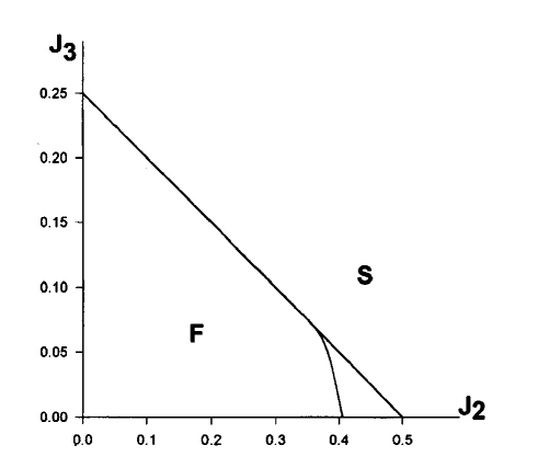
FIG. 1.: $T=0$ phase diagram of the $J_{1},\;J_{2},\;J_{3}$ model with $J_{1}=-1$. The bold line is a boundary between the ferromagnetic and singlet phases in the classical approximation, the bold+thin lines – in present approach.

This method has been applied also to the study of the 2D model with $J_{1}=-1$ and $J_{2},J_{3}>0$ in the vicinity of the phase boundary $2J_{2}+4J_{3}=1$ (Fig.1), which determines the region of stability of the ferromagnetic state in the classical approximation. At $J_{2}<0.36$ the situation is similar to the 1D case [12]. However, at $J_{2}\rightarrow 0.36$ the second order of the perturbation theory in the small parameter describing a deviation from the phase boundary diverges. It proves that quantum fluctuations change the classical phase diagram itself. The energies of one- and two-magnon states are shown in Fig.2 as functions of the parameter $J$ for model (1) ($J_{2}=J$ and $J_{3}=0$ ). The critical values $J_{c}(S_{\max}-1)$ and $J_{c}(S_{\max}-2)$ of the instability of the ferromagnetic state with respect to a creation of one and two magnons are equal to $J_{c}(S_{\max}-1)=1/2$ and $J_{c}(S_{\max}-2)=0.4082$ respectively (two-magnon state energy was found by the numerical solution of the corresponding Schrödinger equation). The difference between $J_{c}(S_{\max}-1)$ and $J_{c}(S_{\max}-2)$ shows that the classical approach is inapplicable to the study of the stability of the ferromagnetic state. In this respect the situation is essentially different from those in the 1D or in the 2D cases at $J_{2}<0.36$, when the critical point $J_{c}$ is independent on the number of magnons and coincides with its classical value. It is natural to assume, that the critical value $J_{c}(S_{\max}-3)$ for model (1) is less than $J_{c}(S_{\max}-2)$, and the critical value $J_{c}(0)$ corresponding to the state with $S=0$ is a true point of the phase transition. So, the classical approximation has proved to be unsuitable for the study of the phase transition in the model (1) and for the determination of the critical value $J_{c}$ and, therefore, another approach is needed.

\begin{picture}(11.0,7.0)\centerline{\hbox{\psfig{angle=0,width=256.0748pt}}} \end{picture}

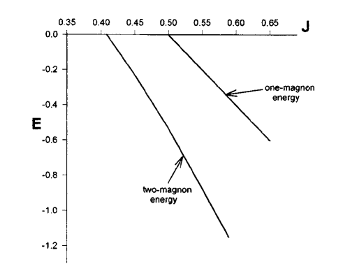
FIG. 2.: Energies of one- and two-magnon states.

One can obtain a crude estimate of the energy and the critical point $J_{c}(0)$ by using a product of the ground state wave functions of two independent antiferromagnetic sublattices as a variational wave function (VWF). This VWF gives for the critical point $J_{c}(0)$ a value:

$$J_{c}=\frac{1}{1-2\varepsilon}\simeq 0.428,$$ (2)

where $\varepsilon$ is the ground state energy per site of the 2D antiferromagnetic Heisenberg model, and we use the most accurate numerical estimations of $\varepsilon=-0.669$ [13,14]. Of course, this approach is too poor, and the obtained value $J_{c}(0)$ is greater than $J_{c}(S_{\max}-2)$.

In the present work we propose a new type of VWF, which allows us to get more accurate estimations of $J_{c}$ and to study the character of the phase transition. This approach is based on a boson representation of the Hamiltonian (1) which is different from the Holstein-Primakoff one. In contrast with the spin wave theory (SWT) the proposed method is variational.

This article is organized as follows. In the next section we demonstrate the method by the application it to the 2D Heisenberg antiferromagnetic model. In section 3 the stability of the ferromagnetic phase of the frustrated model is studied and the data are discussed.

II The method

To illustrate the main features of our approach, let us consider the 2D HAF model:

$$H=\sum_{{\bf n},{\bf a}}{\bf S}_{{\bf n}}\cdot{\bf S}_{{\bf n}+{\bf a}},$$ (3)

where ${\bf n}$ is a site number of the 2D lattice and a vector ${\bf a}$ connects nearest sites.

It is convenient to rotate the local coordinate system of one of sublattices by the angle $\pi$ in XZ plane:

$$H=\sum_{{\bf n},{\bf a}}(-S_{{\bf n}}^{x}\cdot S_{{\bf n}+{\bf a}}^{x}+S_{{\bf n}}^{y}\cdot S_{{\bf n}+{\bf a}}^{y}-S_{{\bf n}}^{z}\cdot S_{{\bf n}+{\bf a}}^{z})$$ (4)

The transformation from spin-operators to bose-ones is defined by:

$$S_{i}^{z}=-\frac{(-1)^{\stackrel{{\scriptstyle\wedge}}{{N}}_{i}}}{2},\qquad S_{i}^{+}=\frac{\theta(\stackrel{{\scriptstyle\wedge}}{{N}}_{i})}{\sqrt{\stackrel{{\scriptstyle\wedge}}{{N}}_{i}}}b_{i}^{+},\qquad S_{i}^{-}=b_{i}\frac{\theta(\stackrel{{\scriptstyle\wedge}}{{N}}_{i})}{\sqrt{\stackrel{{\scriptstyle\wedge}}{{N}}_{i}}},$$ (5)

where $b_{i}^{+}$ are bose-operators, $\stackrel{{\scriptstyle\wedge}}{{N}}_{i}=b_{i}^{+}b_{i}$, and the operator function $\theta(\stackrel{{\scriptstyle\wedge}}{{N}})$ is:

$$\theta(\stackrel{{\scriptstyle\wedge}}{{N}})=\frac{1-(-1)^{\stackrel{{\scriptstyle\wedge}}{{N}}}}{2}$$ (6)

It is evident that this transformation preserves all commutation relations for the spin operators. The states with different numbers of bosons on each site are effectively separated into equivalent unconnected pairs:

$$\left\{\begin{array}[]{ccc}S^{z}\left|2m\right\rangle=-\frac{1}{2}&,\quad S^{+}\left|2m\right\rangle=\left|2m+1\right\rangle&,\quad S^{-}\left|2m\right\rangle=0\\ S^{z}\left|2m+1\right\rangle=\frac{1}{2}&,\quad S^{+}\left|2m+1\right\rangle=0&,\quad S^{-}\left|2m+1\right\rangle=\left|2m\right\rangle\end{array}\right.$$ (7)

As a result of the transformation (5) the Hamiltonian (4) takes the form:

$$H_{b}=\sum_{{\bf n},{\bf a}}\left\{-\frac{(-1)^{\stackrel{{\scriptstyle\wedge}}{{N}}_{{\bf n}}+\stackrel{{\scriptstyle\wedge}}{{N}}_{{\bf n}+{\bf a}}}}{4}-\frac{1}{2}\left(\frac{\theta(\stackrel{{\scriptstyle\wedge}}{{N}}_{{\bf n}})}{\sqrt{\stackrel{{\scriptstyle\wedge}}{{N}}_{{\bf n}}}}b_{{\bf n}}^{+}\frac{\theta(\stackrel{{\scriptstyle\wedge}}{{N}}_{{\bf n+a}})}{\sqrt{\stackrel{{\scriptstyle\wedge}}{{N}}_{{\bf n+a}}}}b_{{\bf n+a}}^{+}+h.c.\right)\right\}$$ (8)

This Hamiltonian, as well as the original one, can not be solved exactly. As a trial wave function for Hamiltonian (8) we choose :

$$\left|\Psi\right\rangle=\exp\left(\frac{1}{2}\sum_{\bf i,j}\Lambda({\bf i}-{\bf j)}\;b_{{\bf i}}^{+}b_{{\bf j}}^{+}\right)\left|0_{b}\right\rangle,$$ (9)

where the function $\Lambda({\bf i}-{\bf j)}$ will be found by the minimization of the total energy.

The vacuum state in Eq.(9) corresponds to the state of the Hamiltonian (4) with all spins pointing down (or corresponds to a ”chess” arrangement of spins for the Hamiltonian (3)).

To calculate the ground state energy we need to calculate expectation values of all terms in the Hamiltonian (8) with respect to VWF (9). At first we calculate the terms corresponding to the spin interactions along the horizontal line (X axe). Owing to the translational symmetry of VWF (9), all of these terms give equal contributions to the energy, and, therefore, it is sufficient to calculate terms corresponding to the interaction ${\bf S}_{1}\cdot{\bf S}_{2}$ in the original Hamiltonian (3), where 1 and 2 are nearest neighbors along the horizontal line.

At first we represent all factors $\frac{1}{\sqrt{\stackrel{{\scriptstyle\wedge}}{{N}}_{j}}}$ in the Hamiltonian (8) in the form:

$$\frac{1}{\sqrt{\stackrel{{\scriptstyle\wedge}}{{N}}_{j}}}=\frac{1}{\sqrt{\pi}}\int\limits_{-\infty}^{\infty}e^{-t_{j}^{2}\stackrel{{\scriptstyle\wedge}}{{N}}_{j}}dt_{j}$$ (10)

Then the expectation value of the second term of the Hamiltonian (8), corresponding to the term $-S_{1}^{x}S_{2}^{x}+S_{1}^{y}S_{2}^{y}$ in the Hamiltonian (4), takes the form:

$$H_{12}^{xy}=-\iint\limits_{-\infty}^{\infty}\frac{dt_{1}dt_{2}}{8\pi}\left[e^{-t_{1}^{2}\stackrel{{\scriptstyle\wedge}}{{N}}_{1}}\left(1-e^{i\pi\stackrel{{\scriptstyle\wedge}}{{N}}_{1}}\right)b_{1}^{+}\;e^{-t_{2}^{2}\stackrel{{\scriptstyle\wedge}}{{N}}_{2}}\left(1-e^{i\pi\stackrel{{\scriptstyle\wedge}}{{N}}_{2}}\right)b_{2}^{+}+h.c.\right]$$ (11)

Thus, we need to calculate expectation values of the type:

$$c_{12}=\frac{\left\langle\Psi\right|\ e^{i\pi(\stackrel{{\scriptstyle\wedge}}{{N}}_{1}+\stackrel{{\scriptstyle\wedge}}{{N}}_{2})}\ \left|\Psi\right\rangle}{\langle\Psi\mid\Psi\rangle}\qquad$$ (12)

and

$$\ d_{12}=\frac{\left\langle\Psi\right|\ (e^{-r_{1}\stackrel{{\scriptstyle\wedge}}{{N}}_{1}}b_{1}^{+}e^{-r_{2}\stackrel{{\scriptstyle\wedge}}{{N}}_{2}}b_{2}^{+}+h.c.)\ \left|\Psi\right\rangle}{\langle\Psi\mid\Psi\rangle},$$ (13)

where $r_{1}$ and $r_{2}$ can be:

$$r_{j}=t_{j}^{2},\qquad\qquad r_{j}=t_{j}^{2}+i\pi\qquad\qquad j=1,2$$ (14)

In order to decompose the boson quadratic form in Eq.(9) we use the Hubbard-Stratanovich transformation. Now, the VWF (9) takes the form:

$$\left|\Psi\right\rangle=\frac{\sqrt{\det\Lambda^{-1}}}{(2\pi)^{N_{0}/2}}\int\limits_{-\infty}^{\infty}\prod\limits_{\bf l}d\eta_{\bf l}\;e^{-\frac{1}{2}\sum\Lambda_{\bf ij}^{-1}\,\eta_{\bf i}\eta_{\bf j}}\;\;e^{\sum\eta_{\bf i}\,b_{\bf i}^{+}}\;\left|0_{b}\right\rangle,$$ (15)

where $N_{0}$ is a number of lattice sites.

Now we can calculate the expectation values (12,13):

$$c_{12}=\frac{\int\limits_{-\infty}^{\infty}\prod\limits_{\bf l}d\xi_{\bf l}d\eta_{\bf l}\;W_{\xi\eta}\;e^{-2(\xi_{1}\eta_{1}+\xi_{2}\eta_{2})}}{\int\limits_{-\infty}^{\infty}\prod\limits_{\bf l}d\xi_{\bf l}d\eta_{\bf l}\;W_{\xi\eta}},$$ (16)

$$d_{12}=\frac{\int\limits_{-\infty}^{\infty}\prod\limits_{\bf l}d\xi_{\bf l}d\eta_{\bf l}\;W_{\xi\eta}\;(\xi_{1}\xi_{2}+\eta_{1}\eta_{2})\;e^{-r_{1}-r_{2}-p_{1}\xi_{1}\eta_{1}-p_{2}\xi_{2}\eta_{2}}}{\int\limits_{-\infty}^{\infty}\prod\limits_{\bf l}d\xi_{\bf l}d\eta_{\bf l}\;W_{\xi\eta}},$$ (17)

where we use the notations:

$$W_{\xi\eta}=exp\left(-\frac{1}{2}\sum\limits_{\bf i,j}\Lambda_{\bf ij}^{-1}\;(\xi_{\bf i}\xi_{\bf j}+\eta_{\bf i}\eta_{\bf j})+\sum\limits_{\bf i}\xi_{\bf i}\eta_{\bf i}\right),$$ (18)

$$p_{j}=1-e^{-r_{j}},\qquad\qquad j=1,2$$ (19)

Using the identity:

$\displaystyle\xi_{1}\xi_{2}+\eta_{1}\eta_{2}=\frac{\partial}{\partial p_{3}}\left[e^{p_{3}(\xi_{1}\xi_{2}+\eta_{1}\eta_{2})}\right]_{p_{3}=0}$

Eqs.(16,17) can be written as:

$$c_{12}=\left\langle e^{-2(\xi_{1}\eta_{1}+\xi_{2}\eta_{2})}\right\rangle_{W_{\xi\eta}}$$ (20)

$$d_{12}=e^{-r_{1}-r_{2}}\cdot\frac{\partial}{\partial p_{3}}\left[\left\langle T_{12}(p,\xi,\eta)\right\rangle_{W_{\xi\eta}}\right]_{p_{3}=0},$$ (21)

where

$$\left\langle\phi(\xi,\eta)\right\rangle_{W_{\xi\eta}}=\frac{\int\limits_{-\infty}^{\infty}\prod\limits_{\bf l}d\xi_{\bf l}d\eta_{\bf l}\;W_{\xi\eta}\;\phi(\xi,\eta)}{\int\limits_{-\infty}^{\infty}\prod\limits_{\bf l}d\xi_{\bf l}d\eta_{\bf l}\;W_{\xi\eta}}$$ (22)

and

$$T_{12}(p,\xi,\eta)=e^{-p_{1}\xi_{1}\eta_{1}-p_{2}\xi_{2}\eta_{2}+p_{3}(\xi_{1}\xi_{2}+\eta_{1}\eta_{2})}$$ (23)

It is convenient to use Hubbard-Stratanovich transformation for (23):

$$\left\langle T_{12}(p,\xi,\eta)\right\rangle_{W_{\xi\eta}}=\int\limits_{-\infty}^{\infty}\prod\limits_{j=1}^{4}dx_{j}\;G_{12}(p,x)\;\left\langle Q_{12}(x,\xi,\eta)\right\rangle_{W_{\xi\eta}},$$ (24)

where

$$Q_{12}(x,\xi,\eta)=exp\left(\frac{ix_{1}+x_{2}}{\sqrt{2}}\xi_{1}+\frac{ix_{1}-x_{2}}{\sqrt{2}}\eta_{1}+\frac{-ix_{3}+x_{4}}{\sqrt{2}}\xi_{2}+\frac{-ix_{3}-x_{4}}{\sqrt{2}}\eta_{2}\right),$$ (25)

$$G_{12}(p,x)=\frac{\exp\left(-p_{2}^{\prime}\frac{x_{1}^{2}+x_{2}^{2}}{2}-p_{1}^{\prime}\frac{x_{3}^{2}+x_{4}^{2}}{2}+p_{3}^{\prime}(x_{1}x_{3}+x_{2}x_{4})\right)}{(2\pi)^{2}\,(p_{1}p_{2}-p_{3}^{2})}$$ (26)

and

$\displaystyle p_{j}^{\prime}=\frac{p_{j}}{p_{1}\,p_{2}-p_{3}^{2}}$

So, there are only linear terms on $\xi$ and $\eta$ in exponent of Eq.(25), and, therefore, we can compute the expectation value $\left\langle Q_{12}(x,\xi,\eta)\right\rangle_{W_{\xi\eta}}$ by diagonalizing $W_{\xi\eta}$.

Using Fourier transformation for $W_{\xi\eta}$ , we obtain:

$$W_{\xi\eta}=\exp\left(-\frac{1}{2}\sum\limits_{\bf k}\left[\omega_{{\bf k}}(\xi_{{\bf k}}\xi_{-{\bf k}}+\eta_{{\bf k}}\eta_{-{\bf k}})-(\xi_{{\bf k}}\eta_{-{\bf k}}+\xi_{-{\bf k}}\eta_{{\bf k}})\right]\right),$$ (27)

where $\omega_{{\bf k}}$ are eigenvalues of the matrix $\Lambda_{{\bf ij}}^{-1}$, and ${\bf k=(}k_{x},k_{y})$.

Diagonalizing the quadratic form in Eq.(27), we find:

$$\left\langle Q_{12}(x,\xi,\eta)\right\rangle_{W_{\xi\eta}}=exp\left(-\frac{x_{1}^{2}+x_{3}^{2}}{2}\sigma^{+}-\frac{x_{2}^{2}+x_{4}^{2}}{2}\sigma^{-}+x_{1}x_{3}\mu_{1-2}^{+}-x_{2}x_{4}\mu_{1-2}^{-}\right),$$ (28)

where we use the notation:

$$\sigma^{\pm} = \pm\frac{1}{N_{0}}\sum\limits_{\bf k}\frac{1}{\omega_{\bf k}\mp 1},$$ (29)

$$\mu_{{\bf n}-{\bf m}}^{\pm} = \pm\frac{1}{N_{0}}\sum\limits_{\bf k}\frac{\cos({\bf k}\cdot{\bf n}-{\bf k}\cdot{\bf m})}{\omega_{\bf k}\mp 1}$$ (30)

Substituting (28) into Eq.(24), we arrive to:

$$\left\langle T_{12}(p,\xi,\eta)\right\rangle_{W_{\xi\eta}}=\iint\limits_{-\infty}^{\infty}\prod\limits_{j=1}^{4}dx_{j}\frac{exp\left(-\frac{1}{2}\sum B_{ij}\,x_{i}\,x_{j}\right)}{(2\pi)^{2}\,(p_{1}p_{2}-p_{3}^{2})}=\frac{\sqrt{\det B^{-1}}}{p_{1}p_{2}-p_{3}^{2}},$$ (31)

where matrix $B_{ij}$ has the form:

$$B_{ij}=\left(\begin{array}[]{cccc}p_{2}^{\prime}+\sigma^{+}&0&-p_{3}^{\prime}-\mu_{1-2}^{+}&0\\ 0&p_{2}^{\prime}+\sigma^{-}&0&-p_{3}^{\prime}+\mu_{1-2}^{-}\\ -p_{3}^{\prime}-\mu_{1-2}^{+}&0&p_{1}^{\prime}+\sigma^{+}&0\\ 0&-p_{3}^{\prime}+\mu_{1-2}^{-}&0&p_{1}^{\prime}+\sigma^{-}\end{array}\right)$$ (32)

Substituting Eqs.(30,31) into (21), we find:

$$d_{12}=e^{-r_{1}-r_{2}}\left(\mu_{1-2}^{+}\;f_{+}^{3}(p_{1},p_{2})\;f_{-}(p_{1},p_{2})-\mu_{1-2}^{-}\;f_{+}(p_{1},p_{2})\;f_{-}^{3}(p_{1},p_{2})\right),$$ (33)

where

$$f_{\pm}(p_{1},p_{2})=\left[(1+p_{1}\sigma^{\pm})(1+p_{2}\sigma^{\pm})-p_{1}p_{2}(\mu_{1-2}^{\pm})^{2}\right]^{-\frac{1}{2}}$$ (34)

There are four terms in (11), corresponding to the different values $r_{1}$, $r_{2}$ and $p_{1}$, $p_{2}$ in (14) and (19).

$$\left\{\begin{array}[]{c}p_{\alpha}=1+\alpha e^{-t_{1}^{2}}\\ q_{\beta}=1+\beta e^{-t_{2}^{2}}\end{array}\right.\qquad\qquad\alpha,\beta=\pm 1$$ (35)

Using the notation (34), Eq.(32) and the definition of functions $f_{+}$ and $f_{-}$ in (33), Eq.(11) can be written as:

$$E_{12}^{xy}=-E_{12}^{x}+E_{12}^{y},$$ (36)

$$E_{12}^{x}=\mu_{1-2}^{+}\iint\limits_{-\infty}^{\infty}\frac{dt_{1}dt_{2}}{8\pi}e^{-t_{1}^{2}-t_{2}^{2}}\sum\limits_{\alpha,\beta=-1}^{1}f_{+}^{3}(p_{\alpha},q_{\beta})\;f_{-}(p_{\alpha},q_{\beta}),$$ (37)

$$E_{12}^{y}=\mu_{1-2}^{-}\iint\limits_{-\infty}^{\infty}\frac{dt_{1}dt_{2}}{8\pi}e^{-t_{1}^{2}-t_{2}^{2}}\sum\limits_{\alpha,\beta=-1}^{1}f_{+}(p_{\alpha},q_{\beta})\;f_{-}^{3}(p_{\alpha},q_{\beta})$$ (38)

We note, that the expectation value $c_{12}$ can be obtained from Eq.(30) by setting $p_{1}=p_{2}=2$ and $p_{3}=0$. Hence, we obtain:

$$E_{12}^{z}=\frac{1}{4}c_{12}=\frac{1}{4}f_{+}(2,2)\,f_{-}(2,2)$$ (39)

The contribution to the energy of the terms corresponding to nearest neighbors along the horizontal line in the Hamiltonian (8) is:

$$E_{12}=-E_{12}^{x}+E_{12}^{y}-E_{12}^{z}$$ (40)

One can verify by rotating the local coordinate systems and repeating the calculations (5-30) for the transformed Hamiltonian, that the values $E_{12}^{x}$ and $E_{12}^{y}$ correspond to expectation values :

$$E_{12}^{x}=\left\langle S_{1}^{x}S_{2}^{x}\right\rangle,\qquad\qquad E_{12}^{y}=\left\langle S_{1}^{y}S_{2}^{y}\right\rangle$$ (41)

The calculation of the expectation values of the terms of the Hamiltonian (8) corresponding to the nearest neighbor interactions along the vertical line (Y axe) ${\bf S}_{1}\cdot{\bf S}_{3}$ can be carried out in the analogy with (9-30). In this case, we must only substitute the functions $\mu_{1-3}^{\pm}$ for $\mu_{1-2}^{\pm}$ into Eqs.(36-38). Then we obtain the contribution to energy of the vertical neighbor terms:

$$E_{13}=-E_{13}^{x}+E_{13}^{y}-E_{13}^{z}$$ (42)

The total energy of Hamiltonian (8) can be written as:

$$E=E_{12}+E_{13}$$ (43)

Thus, we find energy as a function of parameters $\sigma^{\pm},\mu_{1-2}^{\pm},\mu_{1-3}^{\pm}$. These parameters are functions of $\omega({\bf k)}$ [or of $\Lambda({\bf i}-{\bf j})$ in VWF (9)]. Now we need to minimize the energy with respect to $\omega({\bf k)}$:

$$\frac{\partial E}{\partial\omega_{{\bf k}}}=-\frac{a_{1}+b_{1}\cos k_{x}+c_{1}\cos k_{y}}{(\omega_{{\bf k}}-1)^{2}}+\frac{a_{2}+b_{2}\cos k_{x}+c_{2}\cos k_{y}}{(\omega_{{\bf k}}+1)^{2}}=0,$$ (44)

where

$\displaystyle\begin{array}[]{ccc}a_{1}=\frac{\partial E}{\partial\sigma^{+}},&\qquad b_{1}=\frac{\partial E}{\partial\mu_{1-2}^{+}},&\qquad c_{1}=\frac{\partial E}{\partial\mu_{1-3}^{+}},\\ a_{2}=\frac{\partial E}{\partial\sigma^{-}},&\qquad b_{2}=\frac{\partial E}{\partial\mu_{1-2}^{-}},&\qquad c_{2}=\frac{\partial E}{\partial\mu_{1-3}^{-}}\end{array}$

We can define the functional form of $\omega({\bf k)}$ from Eq.(43):

$$\omega({\bf k)=}\frac{1+g({\bf k})}{1-g({\bf k})},$$ (45)

where

$$g({\bf k})=\alpha_{1}\sqrt{\frac{1+\alpha_{2}\cos k_{x}+\alpha_{3}\cos k_{y}}{1+\alpha_{4}\cos k_{x}+\alpha_{5}\cos k_{y}}},$$ (46)

and $\alpha_{i}$ $(i=1,5)$ are variational parameters.

Thus, we reduce the problem of the energy minimization over the variational function $\omega({\bf k)}$ to the energy minimization with respect to five variational parameters $\alpha_{i}$. This procedure has been performed numerically. It gives the final result for 2D HAF:

$$\alpha_{1}=1,\qquad\alpha_{2}=\alpha_{3}=-\alpha_{4}=-\alpha_{5}=-0.445,\qquad E=-0.640$$ (47)

Besides, both terms in Eq.(42) give equal contributions to the energy:

$\displaystyle E_{12}=E_{13}$

Obtained ground state energy for the 2D HAF (3) is 4-4,5% higher than the most accurate results obtained by various numerical techniques [13,14] and is in a good agreement with energies obtained by different VWF methods [15-17].

III Results and discussion

Now we apply the proposed approach to the frustrated model (1). The ground state of the Hamiltonian (1) is ferromagnetic at small $J$. In the classical approximation two-sublattice Neel state is realized at $J>\frac{1}{2}$. The energy of this state is:

$$\frac{E}{N_{0}}=-(J-\frac{1}{2})$$ (48)

A spiral state (the incommensurate phase with the momentum $(Q,Q)$, $\cos Q=\frac{1}{2\cdot J}$) has higher energy at $J>\frac{1}{2}$:

$$\frac{E}{N_{0}}\simeq-(J-\frac{1}{2})^{2}$$ (49)

although it tends to zero at $J\rightarrow\frac{1}{2}$ as well.

Energies of other phases are considerably higher. The energy of the dimer phase, for example, equals to $\frac{E}{N_{0}}=\frac{1}{2}$ at $J=\frac{1}{2}$. Hence, it is natural to consider Neel two-sublattice and the spiral states as main candidates for the ground state at $J>J_{c}$. We will calculate quantum corrections to the classical energy for these states using the VWF (9). Before that, we make the following remark.

The VWF (9) has no rotational symmetry ( it is not the eigenfunction of $S^{2}$), and, therefore, the ground state energy calculated in this approximation depends on the choice of the local coordinate system for the Hamiltonian (1). In other words, if we rotate spin operators ${\bf S}\rightarrow{\bf\varsigma}$ and perform a transformation to bose-operators according to Eq.(5), then, generally speaking, obtained energies will be different in spite of the equivalence of the Hamiltonians $H_{{\bf s}}$ and $H_{{\bf\varsigma}}$. Hence, parameters of the rotation can be considered as variational ones.

For the consideration of the two-sublattice Neel phase let us rotate the coordinate system so that there are the angle $\pi$ in $XZ$ plane between two nearest neighbors on each sublattice (as in the 2D HAF case) and the angle $\varphi$ between sublattices in $XZ$ plane. We will keep the angle $\varphi$ as a variational parameter (we note, that the energy is infinitely degenerated with respect to $\varphi\,$in the classical approximation). In this case, the Hamiltonian (1) takes the form:

$$H= - \sum_{\bf n}[-\frac{1}{2}+\cos\varphi\left(\varsigma_{{\bf n}}^{x}\varsigma_{{\bf n}+{\bf a}_{x}}^{x}+\varsigma_{{\bf n}}^{z}\varsigma_{{\bf n}+{\bf a}_{x}}^{z}-\varsigma_{{\bf n}}^{x}\varsigma_{{\bf n}+{\bf a}_{z}}^{x}-\varsigma_{{\bf n}}^{z}\varsigma_{{\bf n+a}_{z}}^{z}\right)$$ (50)

$$+ \sin\varphi\left(\varsigma_{{\bf n}}^{z}\varsigma_{{\bf n}+{\bf a}_{x}}^{x}-\varsigma_{{\bf n}}^{x}\varsigma_{{\bf n}+{\bf a}_{x}}^{z}-\varsigma_{{\bf n}}^{z}\varsigma_{{\bf n+a}_{z}}^{x}+\varsigma_{{\bf n}}^{x}\varsigma_{{\bf n+a}_{z}}^{z}\right)+\varsigma_{{\bf n}}^{y}\varsigma_{{\bf n}+{\bf a}_{x}}^{y}+\varsigma_{{\bf n}}^{y}\varsigma_{{\bf n+a}_{z}}^{y}]$$ (51)

$$+ J\sum_{\bf n,d}\left(-\varsigma_{{\bf n}}^{x}\varsigma_{{\bf n}+{\bf d}}^{x}+\varsigma_{{\bf n}}^{y}\varsigma_{{\bf n}+{\bf d}}^{y}-\varsigma_{{\bf n}}^{z}\varsigma_{{\bf n}+{\bf d}}^{z}-\frac{1}{4}\right),$$ (52)

where vector ${\bf d}$ connects nearest sites on diagonal line.

Expectation values of the terms in the Hamiltonian (49), such as $\left\langle{\bf\varsigma}_{{\bf n}}^{x}\cdot{\bf\varsigma}_{{\bf m}}^{x}\right\rangle$, $\left\langle{\bf\varsigma}_{{\bf n}}^{y}\cdot{\bf\varsigma}_{{\bf m}}^{y}\right\rangle$ and $\left\langle{\bf\varsigma}_{{\bf n}}^{z}\cdot{\bf\varsigma}_{{\bf m}}^{z}\right\rangle$ are determined by Eqs.(36,37,38) respectively, where $\mu_{{\bf n}-{\bf m}}^{+}$ and $\mu_{{\bf n}-{\bf m}}^{-}$ are defined by Eq.(29).

The VWF (9) contains only terms that involve even numbers of boson operators and, therefore, all expectation values such as $\left\langle{\bf\varsigma}_{{\bf n}}^{x}\cdot{\bf\varsigma}_{{\bf m}}^{z}\right\rangle$ in (49) are equal to zero:

$$\left\langle{\bf\varsigma}_{{\bf n}}^{x}\cdot{\bf\varsigma}_{{\bf m}}^{z}\right\rangle=0$$ (53)

In this case there are nine variational parameters in Eq.(45):

$$g({\bf k})=\alpha_{1}\sqrt{\frac{1+\alpha_{2}\cos k_{x}+\alpha_{3}\cos k_{z}+\alpha_{4}\cos(k_{x}+k_{z})+\alpha_{5}\cos(k_{x}-k_{z})}{1+\alpha_{6}\cos k_{x}+\alpha_{7}\cos k_{z}+\alpha_{8}\cos(k_{x}+k_{z})+\alpha_{9}\cos(k_{x}-k_{z})}}$$ (54)

\begin{picture}(11.0,8.0)\centerline{\hbox{\psfig{angle=0,width=284.52756pt}}} \end{picture}

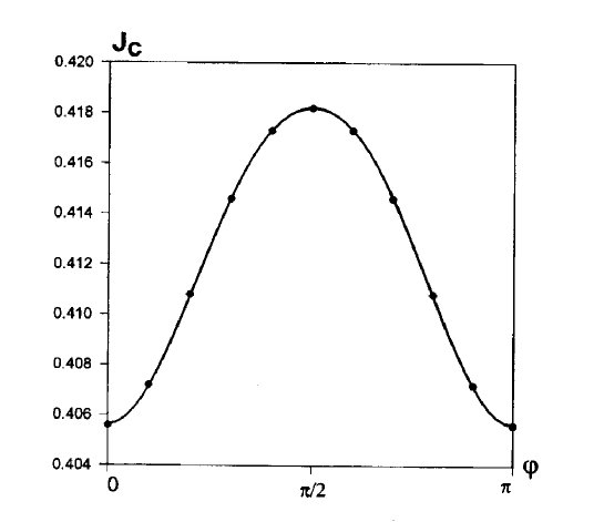
FIG. 3.: The dependence $J_{c}$ on the angle $\varphi$.

The critical value $J_{c}$ is defined by the condition that the ground state energy is negative for $J>J_{c}$. To find $J_{c}$ we minimize the following ratio:

$$J_{c}=\frac{E_{1}}{E_{2}},$$ (55)

where $E_{1}$ and $E_{2}$ are the contributions to the energy from the first and the second terms in the Hamiltonian (49):

$$E=-E_{1}+J\,E_{2}$$ (56)

The dependence of $J_{c}$ on $\varphi$ obtained by a minimization with respect to parameters $\alpha_{i}$ is shown on Fig.3. As it can be seen from Fig.3, the minima of $J_{c}$ are reached at $\varphi=0$ or $\varphi=\pi$. The corresponding states belong to the so called collinear phase. At $\varphi=0$ we have:

$$\alpha_{1}=1,\qquad\alpha_{2}=\alpha_{6}=-0.7,\qquad\alpha_{3}=-\alpha_{7}=0.64,$$ (57)

$$\alpha_{4}=\alpha_{5}=-\alpha_{8}=-\alpha_{9}=-0.36,\qquad J_{c}=0.4056$$ (58)

The calculation of the energy with use of the VWF (9) for the spiral phase can be carried out in a similar way. It turns out that quantum fluctuations do not shift the transition point and change the coefficient in the quadratic dependence in (48) only. The dependences of the energies of the collinear and spiral states are shown on Fig.4. For comparison, we show the spin wave theory results as well. The SWT energy is not a variational one and is defined up to $J=0.52$, where the sublattice magnetization vanishes in the SWT approximation.

\begin{picture}(11.0,8.0)\centerline{\hbox{\psfig{angle=0,width=284.52756pt}}} \end{picture}

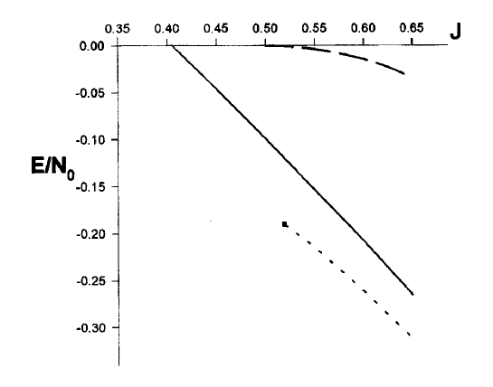
FIG. 4.: Energies of the collinear (solid line) and spiral (dashed) states. Dotted line is the SWT energy of the collinear phase.

Thus, the singlet collinear phase is the ground state of the model (1) for $J>J_{c}$.

A characteristic feature of the considered model (1) is the fact, that the critical value $J_{c}$, (the point of the instability of the ferromagnetic state), depends on $S$ and $J_{c}(S)<J_{c}(S+1)$. In this respect this model differs from the 1D case where $J_{c}$ does not depend on $S$. Such 1D behaviour takes place also in a more general 2D $J_{2}-J_{3}$ model in the vicinity of the classical phase boundary and at $J_{2}<0.36$. In this case, quantum effects do not change the classical boundary of the instability of the ferromagnetic state. The region near the boundary can be considered in the framework of the perturbation theory, and the transition from the ferromagnetic state to the spiral one occurs in this case. The character of the transition changes at $J_{2}>0.36$, and the critical parameter $J_{c}$, corresponding to $E(S)=0$, depends on $S$. In this case the transition from the ferromagnetic to the collinear state is realized. The boundary of the stability of the ferromagnetic phase has a form shown on Fig.1.

In conclusion, we have studied the transition from the ferromagnetic to the singlet state in the 2D frustrated spin model. The transition region is characterized by strong quantum fluctuations and can not be described by the classical approximation. To study the behaviour of the system close to the ferromagnetic boundary we have proposed new approach based on the bozonization of the spin operators. This approach is different from the Holstein-Primakoff method and is variational. We believe that the proposed method can be used to the study of other Heisenberg models with the frustration.

IV Acknowledgments

The authors are grateful to Prof. M.Ya.Ovchinnikova for stimulating discussions. This work is supported by the ISTC under Grant No.015 and in part by RFFR under Grant No.96-03-32186.

REFERENCES

[1] A.Moreo, E.Dagotto, T.Jolicoeur and J.Riera, Phys.Rev.B 42
(1990) 6238
[2] P.Locher, Phys.Rev.B 41 (1990) 2537
[3] E.Dagotto and A.Moreo, Phys.Rev.B 39 (1989) 4744
[4] P.Chandra and B.Doucot, Phys.Rev.B 38 (1988) 9335
[5] A.V.Chubukov and T.Jolicoeur, Phys.Rev.B 44 (1991) 12050
[6] P.Chandra, P.Coleman and A.I.Larkin, J.Phys.Condens.Matter 2
(1990) 7933
[7] D.J.J.Farnell and J.B.Parkinson, J.Phys.Condens.Matter 6 (1994)
5521