Semiclassical approach to the thermodynamics of spin chains

Abstract

Using the PQSCHA semiclassical method, we evaluate thermodynamic quantities of one-dimensional Heisenberg ferro- and antiferromagnets. Since the PQSCHA reduces their evaluation to classical-like calculations, we take advantage of Fisher’s exact solution to get all results in an almost fully analytical way. Explicitly considered here are the specific heat, the correlations length and susceptibility. Good agreement with Monte Carlo simulations is found for $S>1$ antiferromagnets, showing that the relevance of the topological terms and of the Haldane gap is significant only for the lowest spin values and temperatures.

Several applications to condensed matter systems have demonstrated the usefulness of the improved [1, 2] effective potential approach [3]; its generalized version for non standard Hamiltonian, the so called pure-quantum self-consistent harmonic approximation (PQSCHA) [4, 5], has also been successfully applied to different spin systems.

We consider here the one-dimensional isotropic Heisenberg model Hamiltonian,

$${\cal H}=\pm\frac{J}{2}\sum_{{\boldsymbol{j}}\,{\boldsymbol{\delta}}}{\boldsymbol{S}}_{\boldsymbol{j}}{\cdot}{\boldsymbol{S}}_{{\boldsymbol{j}}+{\boldsymbol{\delta}}}~{},$$ (1)

with the exchange interaction $J>0$ restricted to nearest-neighbour sites of a simple cubic $d$-dimensional lattice; the sign $-$ refers to the ferromagnet (FM), $+$ to the antiferromagnet (AFM). The thermodynamic quantities of this model were successfully calculated for two- [6, 7] and three-dimensional [8] magnets, both of which are characterized by a ground state that can be obtained perturbatively starting from the classical-like minimum-energy configuration.

In one dimension the situation is largely different and the ferro- and antiferromagnets, at variance with the classical case where both models are mapped onto the classical non linear Schrödinger equation, behave in a markedly different way. In fact, ferromagnets do not present any peculiarity, being their (ordered) ground state, as in higher dimension, the quantum counterpart of the classical minimum-energy configuration. The relevant excitations, both linear and non-linear, which contributes to the thermodynamic properties and destroy the long-range order at any finite temperature, are basically the same in the quantum and in the classical case. The absence of long-range order at any $T\neq 0$ [9] implies that the linear excitations spectrum should be considered only up to wavelengths of the order of the correlation length $\xi(T)$.

Quantum effects have a much more apparent impact on the qualitative behaviour of antiferromagnets. Its ground state cannot be obtained perturbatively from the Néel configuration, and the relevant quantum excitations are completely different from the classical ones. Moreover, as firstly suggested by Haldane [10, 11], integer and half-integer spin chains display a qualitatively different low-temperature behaviour, which arises from a topological term in the path-integral description of spin systems. For half-integer spins, the interference term leads to gapless excitations, while the Haldane gap appears for integer $S$. However, these effects should rapidly disappear for increasing spin value, as the interference becomes less destructive and the gap vanishes exponentially.

Hence, in one dimensional magnets should also exist regimes where semiclassical methods can be sensibly applied, i.e., when the spin length and/or the temperature increase and the classical behaviour is approached. In such regimes, the PQSCHA is a good tool for calculating thermodynamic quantities and should be very competitive in comparison with other semiclassical ones, as, for instance, the theory based on the use of real-space coherent states that has been recently introduced [12]. Indeed, by the PQSCHA most calculations can be performed analytically, and with a full quantum inclusion of the linear excitations in wave-vector space.

The final outcome of the application of the PQSCHA to Heisenberg models is that the free energy of the quantum model described by Eq. (1) is given by the the free energy of the effective classical Heisenberg Hamiltonian,

$${\cal H}_{\rm{eff}}=\pm\frac{1}{2}J{\widetilde{S}}^{2}\,\theta^{4}(t)\sum_{{\boldsymbol{j}}\,{\boldsymbol{\delta}}}{\boldsymbol{s}}_{\boldsymbol{j}}{\cdot}{\boldsymbol{s}}_{{\boldsymbol{j}}+{\boldsymbol{\delta}}}+NJ{\widetilde{S}}^{2}{\cal G}(t)~{},$$ (2)

whose thermodynamic properties are exactly known after the work by Fisher [13]. In Eq. (2) ${{\boldsymbol{s}}_{\boldsymbol{j}}}$ are unit vectors, ${\widetilde{S}}=S+1/2$ plays the role of the ‘classical’ spin length and $J{\widetilde{S}}^{2}$ that of the overall energy scale: we hence define $t=k_{B}T/J{\widetilde{S}}^{2}$ as the reduced temperature. The temperature- and spin-dependent parameters $\theta(t)$ and ${\cal G}(t)$ account for the effects of the pure-quantum fluctuations. Their explicit expressions are:

$$\theta^{2}(t) = 1-\frac{{\cal D}}{2}~{},$$ (3)

$${\cal G}(t) = \frac{t}{N}\sum_{k}\ln\frac{\sinh f_{k}}{\theta^{2}f_{k}}-\frac{z}{2}\kappa^{2}(t)\,{\cal D}~{}.$$ (4)

It is worthwhile pointing out that the first term of ${\cal G}(t)$ restores the quantum free energy of the linear excitations [5]. The renormalization coefficient ${\cal D}(t)$ reads

$${\cal D}={1\over N{\widetilde{S}}}\,\sum_{\boldsymbol{k}}\Big{(}\coth f_{\boldsymbol{k}}{-}\frac{1}{f_{\boldsymbol{k}}}\Big{)}\times\!\left\{\begin{array}[]{ll}\sqrt{1-\gamma_{\boldsymbol{k}}^{2}}{}{}&\mbox{(AFM)}\\ (1-\gamma_{\boldsymbol{k}})&\mbox{(FM)}\end{array}\right.,$$ (5)

and represents indeed the pure-quantum nearest-neighbour transverse spin fluctuations in self-consistent Gaussian approximation. This essential renormalization coefficient of the PQSCHA for Heisenberg models, as well as the connected quantities $\theta^{2}(t)$ and ${\cal G}(t)$, are global parameters, i.e., they take into account the quantum effects only on average, so that the details of the excitation spectrum are smeared out. Furthermore, $f_{\boldsymbol{k}}=(\hbar\omega_{\boldsymbol{k}})/(2k_{B}T)=\widetilde{\omega}_{\boldsymbol{k}}/2{\widetilde{S}}{t}$, where

$$\widetilde{\omega}_{\boldsymbol{k}}=\left\{\begin{array}[]{ll}z\kappa^{2}\,\sqrt{1-\gamma_{\boldsymbol{k}}^{2}}{}{}&\mbox{(AFM)}\\ z\kappa^{2}\,(1-\gamma_{\boldsymbol{k}})&\mbox{(FM)}\end{array}\right.,$$ (6)

are the dimensionless spin-wave frequencies, whose renormalization factor $\kappa^{2}(t)={1\over 2}\Big{(}\theta^{2}+\sqrt{\theta^{4}-{4}t\varepsilon/z}\Big{)}$ is calculated by taking into account only the thermal fluctuations with $|{\boldsymbol{k}}|>\pi/\xi(t)$, so that $\varepsilon=1-1/\xi$ for the one-dimensional system. We point out that the contributions to the pure-quantum renormalization coefficient (5) are weighted by the Langevin function $\coth{f}_{\boldsymbol{k}}-f_{\boldsymbol{k}}^{-1}$, so that the major role is played by the high-frequency (short wavelength) excitations, which are just those that survive in spite of the absence of long-range order. The PQSCHA in the low-coupling approximation [4, 6, 7] employed to derive Eq. (2) neglects contributions of order ${\cal D}^{2}$ so that ${\cal D}$ must be small compared to one.

Using the exact results for the classical one-dimensional Heisenberg model of Ref. [13], we can thus easily write an analytical expression for the free energy per spin of the quantum spin chain within the PQSCHA:

$${f\over J{\widetilde{S}}^{2}}={\cal G}(t,S)-t\ln\left[\sinh\left({\theta^{4}(t,S)\over t}\right)\cdot{t\over\theta^{4}(t,S)}\right]~{}.$$ (7)

The other macroscopic thermodynamic quantities, e.g. internal energy and specific heat, can be easily obtained from this equation by (numerical) derivation, taking care of the $t$-dependence of ${\cal G}$ and $\theta$, which prevents us from using directly the expressions of Ref. [13] in evaluating such quantities. One can also obtain the spin correlation function and the susceptibility by means of the formulas reported in Ref. [7], where it is shown also how the correlation length $\xi(t)$ is simply related to its classical counterpart only by the change of the temperature scale involved in the renormalization of the exchange constant,

$$\xi(t)=\xi_{\rm{cl}}\big{(}t/\theta^{4}(t)\big{)}~{}.$$ (8)

This formula is of remarkable simplicity, especially when one notices that $\xi_{\rm{cl}}(t)$ has a very simple analytical expression [13],

$$\xi_{\rm{cl}}(t)=\big{[}-\ln(\coth t^{-1}-t)\big{]}^{-1}~{}.$$ (9)

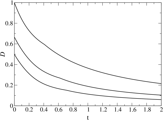
FIG. 1.: Pure-quantum renormalization coefficient ${\cal{D}}(t,S)$ vs. temperature $t=T/J{\widetilde{S}}^{2}$, for the Heisenberg FM chain. From the uppermost curve, the spin values are $S=1/2$, $S=1$ and $S=3/2$.

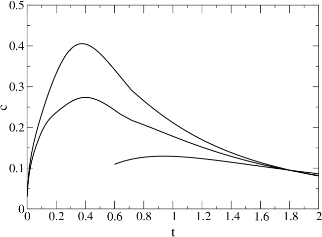
FIG. 2.: Specific heat $c(t)$ of the Heisenberg FM chain for $S=1/2$, $S=1$ and $S=3/2$, respectively, starting from the lower-most curve.

In principle, the PQSCHA approach should work well for the one-dimensional Heisenberg FM, because:  i) their ground state is ordered and is an eigenstate of $S^{z}_{\rm{tot}}=\sum_{i}S_{i}^{z}$;  ii) the absence of long-range order at any finite temperature is due to nonlinear excitations, which can be well treated in semiclassical ($1/S$-expansion) approximation;  iii) the pure-quantum fluctuations related to the linear excitations are accounted for through the coefficient ${\cal D}(t)$. Therefore, the only limitation we should care of for the FM is a possible too high value of ${\cal D}$: we shall assume that the condition ${\cal D}\lesssim{0.5}$ must be satisfied to get reliable results. As shown in Fig. 1 this occurs at any temperature for $S\geq{3/2}$. As for lower values of $S$ it is apparent that for $S=1$ the approach can be used in a wide range of temperatures starting from $t\gtrsim{0.25}$; on the other hand, the strongest quantum case, $S=1/2$, cannot be well described except for very high temperatures $t\gtrsim{1}$.

Unfortunately, to the best of our knowledge, reference data on one-dimensional Heisenberg ferromagnets are not available for intermediate spin values, and we found only rather old ones for $S=1/2$[14, 15]. However it could be appealing to derive some thermodynamic quantities by means of the effective Hamiltonian (2) and Eq. (7). The specific heat of the FM spin chain is shown in Fig. 2 for spin values $S=1/2$, $S=1$ and $S=3/2$. Comparing with Fig. 1 we see why the curve for $S=1/2$ is truncated at $t\simeq{1}$: for higher temperature the behaviour of $C(t)$ is in agreement with the available numerical data[14, 15] .

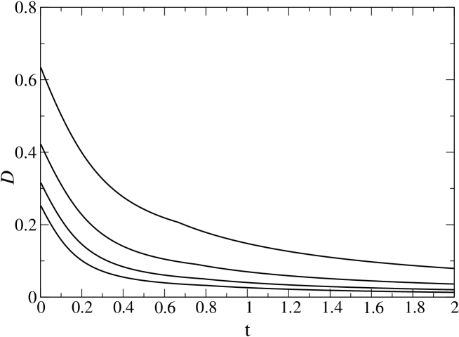
FIG. 3.: Pure-quantum renormalization coefficient ${\cal D}(t,S)$ vs. temperature $t=T/J{\widetilde{S}}^{2}$, for the Heisenberg AFM chain. From the uppermost curve the spin values are $S=1/2$, $1$, $3/2$, and $2$.

Turning to antiferromagnets, the temperature behaviour of ${\cal D}(t)$ is shown in Fig. 3. Using the same criterion as above, we can deduce that the PQSCHA should work well for any temperatures for $S\geq{1}$ while its validity is confined to $t\gtrsim{0.15}$ for $S=1/2$. However, we must recall that the afore-mentioned quantum effects which strongly modify the nature of the ground state and lead to the Haldane gap, cannot be accounted for by any semiclassical approach, so that we do not expect that peculiar quantum properties at very low temperature and low values of the spin could be reproduced within the PQSCHA. Instead the PQSCHA is expected to give good results when the spin becomes larger and larger approaching the classical AFM Heisenberg model.

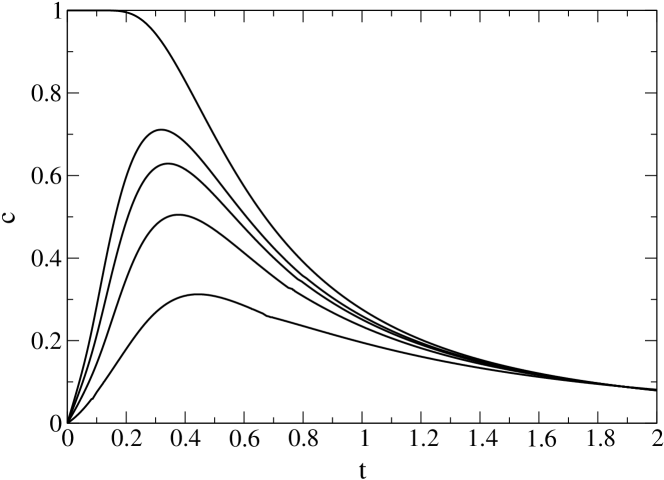
FIG. 4.: Specific heat $c(t)$ of the Heisenberg AFM chain for $S=1/2$, $1$, $3/2$, $2$, and $\infty$ (classical limit), respectively, starting from the lower-most curve.

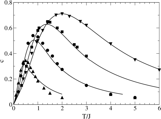
FIG. 5.: Comparison of the specific heat $c(t)$ of the Heisenberg AFM chain, plotted vs. $T/J=t{\widetilde{S}}^{2}$, with numerical simulation data for $S=1/2$ [18], $S=1$ [16], $S=3/2$ [18] and $S=2$ [17].

The results for the specific heat plotted in Figs. 4 and 5 seem to confirm this prediction for the thermodynamic quantities. The comparison with the existing quantum Monte Carlo [16, 17] and transfer-matrix Renormalization Group [18] data shows that the agreement improve for larger spin and can be considered very good almost at all temperature already for $S=3/2$.

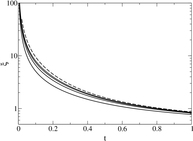
FIG. 6.: Correlation length $\xi(t)$ of the AFM Heisenberg chain for $S=1/2$, $S=1$, $S=3/2$ and $S=2$, respectively, starting from the lower-most curve; the dashed line is the classical result.

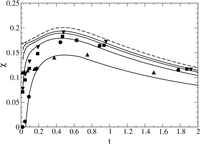
FIG. 7.: Comparison of the uniform susceptibility $\chi(t)$ of the AFM Heisenberg chain with Quantum Monte Carlo simulation data [19]. Spin values are $S=1/2$ (line and upward triangles), $S=1$ (line and circles), $S=3/2$ (line and squares) and $S=2$ (line and downward triangles), respectively, starting from the lower-most curve; the dashed line is the classical result.

In Figs. 6 and 7 we show the PQSCHA results for the correlation length $\xi(t)$ and the uniform susceptibility $\chi(t)$ of the AFM chain. The latter quantity has been shown to be particularly sensitive to test the peculiar quantum effects related to the Haldane gap; nevertheless, Fig. 7 clearly shows that a semiclassical approach like the PQSCHA compares well with numerical data not only where the classical regime is already approached, but also in the intermediate temperature range, where the curves for low spin values already are clearly different from the classical behaviour; only the very low temperature behaviour can not be, as expected, reproduced.

The conclusion is that the thermodynamic quantities of the Heisenberg AFM are not strongly affected by the consequences of the Haldane ground state at intermediate and high temperatures. Small differences appear only at the lowest values of the spin and from the point of view of the PQSCHA it is difficult to ascertain if they are due to the ”Haldane effects” or to the rather large value of ${\cal D}$. On the other hand, it is curious to note that the Haldane conjecture was theoretically proven for large $S$ – where the role of the topological term decreases and the gap is exponentially vanishing, giving negligible quantitative contributions to the thermodynamics.

REFERENCES

- [1] R. Giachetti and V. Tognetti, Phys. Rev. Lett. 55, 912 (1985).
- [2] R. P. Feynman and H. Kleinert, Phys. Rev. A 34, 5080 (1986).
- [3] R. P. Feynman and A. R. Hibbs, Quantum Mechanics and Path Integrals (Mc Graw Hill, New York, 1965).
- [4] A. Cuccoli, V. Tognetti, P. Verrucchi, and R. Vaia, Phys. Rev. A 45, 8418 (1992).
- [5] A. Cuccoli et al., J. Phys.: Condens. Matter 7, 7891 (1995).
- [6] A. Cuccoli, V. Tognetti, P. Verrucchi, and R. Vaia, Phys. Rev. Lett. 79, 1584 (1997).
- [7] A. Cuccoli, V. Tognetti, P. Verrucchi, and R. Vaia, Phys. Rev. B 56, 14456 (1997).
- [8] A. Cuccoli, R. Maciocco, and R. Vaia, In preparation (1999).
- [9] N. D. Mermin and H. Wagner, Phys. Rev. Lett. 17, 1133 (1966).
- [10] F. D. M. Haldane, Phys. Lett. A93, 464 (1983).
- [11] F. D. M. Haldane, Phys. Rev. Lett. 50, 1153 (1983).
- [12] K. Kladko, P. Fulde, and D. A. Garanin, Europhys. Lett. 46, 425 (1999); D. A. Garanin, K. Kladko, P. Fulde, cond-mat/9905061.
- [13] M. E. Fisher, Am J. Phys. 32, 343 (1964).
- [14] J. C. Bonner and M. E. Fisher, Phys. Rev. 135, A640 (1964).
- [15] J. J. Cullen and D. P. Landau, Phys. Rev. B 27, 297 (1983).
- [16] S. Yamamoto and S. Miyashita, Phys. Rev. B 48, 9528 (1993).
- [17] S. Yamamoto, Phys. Rev B 53, 3364 (1996).
- [18] T. Xiang, Phys. Rev. B 58, 9142 (1998).
- [19] Y. J. Kim, M. Greven, U. Wiese, and R. J. Birgeneau, Eur. Phys. J. B 4, 291 (1998).