Random antiferromagnetic quantum spin chains:
Exact results from scaling of rare regions

Abstract

We study $XY$ and dimerized $XX$ spin-$1/2$ chains with random exchange couplings by analytical and numerical methods and scaling considerations. We extend previous investigations to dynamical properties, to surface quantities and operator profiles, and give a detailed analysis of the Griffiths phase. We present a phenomenological scaling theory of average quantities based on the scaling properties of rare regions, in which the distribution of the couplings follows a surviving random walk character. Using this theory we have obtained the complete set of critical decay exponents of the random $XY$ and $XX$ models, both in the volume and at the surface. The scaling results are confronted with numerical calculations based on a mapping to free fermions, which then lead to an exact correspondence with directed walks. The numerically calculated critical operator profiles on large finite systems $(L\leq 512)$ are found to follow conformal predictions with the decay exponents of the phenomenological scaling theory. Dynamical correlations in the critical state are in average logarithmically slow and their distribution show multi-scaling character. In the Griffiths phase, which is an extended part of the off-critical region average autocorrelations have a power-law form with a non-universal decay exponent, which is analytically calculated. We note on extensions of our work to the random antiferromagnetic $XXZ$ chain and to higher dimensions.

I Introduction

Quantum spin chains exhibit many interesting physical properties at low temperatures which are related to the behavior of their ground state and low-lying excitations. In this context one should mention quasi-long-range-order (QLRO), topological order and quantum phase transitions, which have purely quantum mechanical origin. Considering isotropic antiferromagnetic chains for integer spins there is a gap, whereas half integer spin chains are gap-less[1]. However, alternating couplings in spin-$1/2$ chains yield a dimerized ground state that has physical properties similar to the spin-$1$ chain: there is a finite gap, spatial correlations decay exponentially and there is string topological order.

Randomness may have a profound effect on the physical properties of quantum spin chains, as demonstrated by recent analytical and numerical studies[2]. As an interplay of randomness and quantum fluctuations there are new exotic phases in disordered quantum spin chains, which are not present in classical random or pure quantum systems. It has been noticed, that pure gap-less systems are generally unstable against weak randomness[3, 4], whereas for gaped systems a finite amount of disorder is necessary to destroy the gap[5, 6, 7] (but see also[8]).

Among the theoretical methods developed for disordered quantum spin chains one very powerful procedure is the renormalization group (RG) approach introduced by Dasgupta and Ma[3]. This RG method, which is expected to be asymptotically exact at large scales, i.e. close to critical points, has been applied for a number of random quantum systems. The fixed point distribution of the RG transformation has been obtained analytically for some random quantum spin chains, among others for the transverse Ising spin chain[9], the spin-$1/2$ Heisenberg and related spin chains with random antiferromagnetic couplings[4]. On the other hand some other one-dimensional problems ($S=1/2$ Heisenberg chain with mixed ferromagnetic and antiferromagnetic couplings[10, 11], $S=1$ antiferromagnetic chain with and without biquadratic exchange[5, 6, 7], etc.), as well as higher dimensional random quantum systems[12] have been studied by numerical implementation of the RG procedure. Comparing the RG results with those obtained by direct numerical evaluation of the singular quantities[13, 14, 15, 16] and by other exact[17, 15] and numerical methods one has obtained a good agreement in the vicinity of the critical point.

There are, however, other interesting singular quantities, which are not accessible by the RG method. We mention, among others, the dynamical correlations[18] and the behavior of the system far away from the critical point in the Griffiths phase[19], which denotes an extended region of the parameter space around the critical point. In the Griffiths phase the system is gap-less, thus dynamical correlations decay with a power-law, however there is long-range-order with exponentially decaying spatial correlations. For the random quantum Ising chain dynamical correlations, both at the critical point and in the Griffiths phase have been exactly determined[20, 21, 22] using a mapping to the Sinai model[23], i.e. random walk in a random environment.

In this paper we are going to study the $S=1/2$ disordered $XX$ and $XY$ spin chains by analytical and numerical methods and by phenomenological scaling theory. The RG treatment of the problem by Fisher[4] predicts the antiferromagnetic random $XX$ fixed point to control the critical behavior of the antiferromagnetic Heisenberg ($XXX$) model, too. Furthermore, for random isotropic chains the RG approach predicts QLRO, thus the average spatial correlations of different components of the spin decay with a power-law. In this so called random singlet (RS) phase all spins are paired and form singlets, however, the distance between the two spins in a singlet pair can be arbitrarily large. Then these weakly coupled singlets dominate the average correlation function, therefore all components of the correlation function are predicted to decay with the same exponent.

Leaving the critical state by introducing either anisotropy or dimerization, randomness will drive the system into the Griffiths phase. As shown by an RG analysis[5], applicable in the vicinity of the RS fixed point, the Griffiths phase is characterized by the dynamical exponent, $z$, defined by the asymptotic relation between relevant time ($t_{r}$) and length scales ($\xi$) as

$$t_{r}\sim\xi^{z}\;.$$ (1)

The dynamical exponent is predicted to be a continuous function of the quantum control parameter (anisotropy or dimerization) and the singular behavior of different physical quantities (specific heat, susceptibility, etc.) are all expected to be related to the value of the dynamical exponent.

The RG predictions by Fisher[4] and others[5] have been confronted with results of numerical studies[24, 25, 26], especially in the RS phase of isotropic chains, but some cross-over functions of correlations have also been studied in the Griffiths phase. In the RS phase some numerical results are controversial: in earlier studies[25] a different scenario from the RG picture is proposed (in particular with respect to the transverse correlation function), later investigations on larger finite systems have found satisfactory agreement with the RG predictions[26], although the finite-size effects were still very strong.

In the present paper we extend previous work in several directions. Here we consider open chains and study both bulk and surface quantities, as well as end-to-end correlations. We develop a phenomenological theory which is based on the scaling properties of rare events and determine the complete set of critical decay exponents. We calculate numerically (off-diagonal) spin-operator profiles, whose scaling properties are related to (bulk and surface) decay exponents[27] and compare the profiles with predictions of conformal invariance. Another new feature of our work is the study of dynamical correlations, both at the critical point and in the Griffiths phase. Finally, we perform a detailed analytical and numerical study of the Griffiths phase and calculate, among others, the exact value of the dynamical exponent, $z$ in Eq.(1).

The structure of the paper is the following. The model and its free-fermion representation are presented in Section 2. A phenomenological theory based on the scaling behavior of rare events is developed in Section 3. Results in the critical state, where there is quasi-long-range order in the chains is presented in Section 4, whereas the Griffiths phase is studied in Section 5. We discuss the extensions of our results to random antiferromagnetic $XXZ$ chains and to higher dimensions in the final Section, whereas some technical calculations are presented in the Appendices.

II The model and its free-fermion representation

A The $XY$ and $XX$ models

We consider an open $XY$ chain (i.e. with free boundary conditions) with $L$ sites described by the Hamiltonian:

$$H=\sum_{l=1}^{L-1}\left(J_{l}^{x}S_{l}^{x}S_{l+1}^{x}+J_{l}^{y}S_{l}^{y}S_{l+1}^{y}\right)\;,$$ (2)

where the $S_{l}^{\mu}$ ($\mu=x,y$) are spin-$1/2$ operators and the couplings ($J_{l}^{\mu}>0$) are independent random variables with distributions $\pi^{\mu}(J^{\mu})$. The quantum control parameter is the average anisotropy defined as:

$$\delta_{a}={[\ln J^{x}]_{\rm av}-[\ln J^{y}]_{\rm av}\over{\rm var}[\ln J^{x}]+{\rm var}[\ln J^{y}]}\;,$$ (3)

where ${\rm var}(x)$ is the variance of random variable $x$ and $[\dots]_{\rm av}$ denotes average over quenched disorder. For $\delta_{a}>0~{}(<0)$ there is long-range-order in the $x$ ($y$) direction, i.e. $\lim_{r\to\infty}[C^{\mu}(r)]_{\rm av}\neq 0$, where

$$[C^{\mu}(r)]_{\rm av}=[\langle 0|S_{l}^{\mu}S_{l+r}^{\mu}|0\rangle]_{\rm av}\;,$$ (4)

and for $\delta_{a}=0$ the system is in a critical state with quasi-long-range-order, where correlations decay algebraically, i.e.

$$[C^{\mu}(r)]_{\rm av}\sim r^{-\eta^{\mu}}\;.$$ (5)

In the $XX$ model, where the $x$ and $y$ couplings are correlated as $J_{l}^{x}=J_{l}^{y}=J_{l}$, we introduce alternation such that even ($e$) and odd ($o$) couplings, connecting the site $2i,2i+1$ and $2i-1,2i$, respectively, are taken from distributions $\rho^{e}(J_{e})$ and $\rho^{o}(J_{o})$, respectively. For the $XX$ model the quantum control parameter is the average dimerization defined as:

$$\delta_{d}={[\ln J_{o}]_{\rm av}-[\ln J_{e}]_{\rm av}\over{\rm var}[\ln J_{o}]+{\rm var}[\ln J_{e}]}\;.$$ (6)

The RS phase is at $\delta_{d}=0$, whereas $\delta_{d}\neq 0$ corresponds to the random dimer (RD) phase. Throughout the paper we use two types of random distributions, both for the $XY$ and $XX$ models. For the $XY$ model with the binary distribution the $J^{x}$ couplings can take two values $\lambda>1$ and $1/\lambda$ with probability $p$ and $q=1-p$, respectively, while the couplings $J^{y}$ are constant:

$$\pi^{x}(J^{x}) = p\delta(J^{x}-\lambda)+q\delta(J^{x}-\lambda^{-1});$$ (7)

$$\pi^{y}(J^{y}) = \delta(J^{y}-J^{y}_{0})\;.$$ (8)

At the critical point $(p-q)\ln\lambda=\ln J^{y}_{0}$. The uniform distribution is defined via

$$\pi^{x}(J^{x}) = \cases{1,&for $0<J^{x}<1$\cr 0,&otherwise\cr}\;$$ (9)

$$\pi^{y}(J^{y}) = \cases{(J^{y}_{0})^{-1},&for $0<J^{y}<J^{y}_{0}$\cr 0,&otherwise\cr}\;.$$ (10)

and the critical point is at $J^{y}_{0}=1$.

For the $XX$ model the corresponding distributions $\rho^{e}(J^{e})$ and $\rho^{o}(J^{o})$ follows from the correspondences:

$$J^{x}\to J^{e},~{}~{}J^{y}\to J^{o},$$ (11)

$$\pi^{x}(J^{x})\to\rho^{e}(J^{e}),~{}~{}\pi^{y}(J^{y})\to\rho^{o}(J^{o})\;.$$ (12)

Note that the critical points of the two models ($\delta_{a}=0$ and $\delta_{d}=0$, respectively) are not equivalent due to the different disorder correlations.

B The $XY$ chain and the directed walk model

Using the Jordan-Wigner transformation, the $XY$ model Hamiltonian in Eq.(2) can be rewritten as a quadratic form in fermion operators. It is then diagonalized through a canonical transformation which gives

$$H=\sum_{q=1}^{L}\epsilon_{q}(\eta_{q}^{+}\eta_{q}-{1\over 2})\;.$$ (13)

The fermion excitations are non-negative and satisfy the set of equations

$$\epsilon_{q}\Psi_{q}(l) = J^{y}_{l-1}\Phi_{q}(l-1)+J_{l}^{x}\Phi_{q}(l+1)$$ (14)

$$\epsilon_{q}\Phi_{q}(l) = J^{x}_{l-1}\Psi_{q}(l-1)+J_{l}^{y}\Psi_{q}(l+1);\,$$ (15)

with the boundary conditions $J^{x}_{L}=J^{y}_{L}=0$. The vectors $\Phi_{q}$’s and $\Psi_{q}$’s which are related to the coefficients of the canonical transformation are normalized. They enter into the expressions of correlation functions and thermodynamic quantities.

Usually one proceeds[28] by eliminating either $\Psi_{q}$ or $\Phi_{q}$ in Eqs.(15) and the excitations are deduced from the solution of quadratic equations. This last step can be avoided by introducing a $2L$-dimensional vector $V_{q}$ with components:

$$V_{q}(4l-3)=\Phi_{q}(2l-1),~{}~{}~{} V_{q}(4l-2)=\Psi_{q}(2l-1),$$ (16)

$$V_{q}(4l-1)=\Psi_{q}(2l),~{}~{}~{} V_{q}(4l)=\Phi_{q}(2l);\,$$ (17)

and noticing that the relations in Eqs.(15) then correspond to the eigenvalue problem of the matrix:

  

$$T=\left(\matrix{0&0&J_{1}^{y}&&&&&&&\cr 0&0&0&J_{1}^{x}&&&&&&\cr J_{1}^{y}&0&0&0&J_{2}^{x}&&&&&\cr&J_{1}^{x}&0&0&0&J_{2}^{y}&&&&\cr&&J_{2}^{x}&0&0&0&J_{3}^{y}&&&\cr&&&J_{2}^{y}&0&0&0&\ddots&&\cr&&&&\ddots&\ddots&\ddots&\ddots&J_{L-1}^{y}&\cr&&&&&J_{L-2}^{y}&0&0&0&J_{L-1}^{x}\cr&&&&&&J_{L-1}^{y}&0&0&0\cr&&&&&&&J_{L-1}^{x}&0&0\cr}\right)$$ (18)

  

The matrix $T$ can be interpreted as the transfer matrix (TM) of a directed walk (DW) problem on four inter-penetrating, diagonally layered square lattices. Each walker makes steps with weights $J_{l}^{x}$ and $J_{l}^{y}$ between next-neighbor sites on one of the four square lattices and the walk is directed in the diagonal direction (see Fig. 1).

According to Eqs.(15), changing $\Phi_{q}$ into $-\Phi_{q}$ in $V_{q}$, the eigenvector corresponding to $-\epsilon_{q}$ is obtained. Thus all information about the DW and the XY model is contained in that part of the spectrum with $\epsilon_{q}\geq 0$. Later on we shall consider this sector. We note that similar correspondence has been established earlier between the DW and the transverse-field Ising model (TIM)[29].

The eigenvalues of $T$ in (18) are of two classes. For $q=2i-1,~{}i=1,2,\dots,L$ the odd components of the eigenvectors are zero, i.e. $V_{2i-1}(2j)=0,~{}j=1,2,\dots,L$, whereas for the other class with $q=2i$ the even components are zero, $V_{2i}(2j-1)=0$. Consequently $T$ can be expressed as a direct product $T=T_{\sigma}\bigotimes T_{\tau}$, where the trigonal matrices $T_{\sigma}$ , $T_{\tau}$ of size $L\times L$ represent transfer matrices of directed walks. As a result one has to diagonalize these two matrices of size $L\times L$. Thus for chains with even number of sites, $L=2N$, the two classes of eigenvectors are given in terms of the variables $\Phi$ and $\Psi$ via:

$$\begin{array}[]{llclcl}\epsilon_{2k-1}:&\Phi_{2k-1}(2j)&=&\Psi_{2k-1}(2j-1)&=&0\\ \epsilon_{2k}:&\Phi_{2k}(2j-1)&=&\Psi_{2k}(2j)&=&0\end{array}$$ (19)

for $i,j=1,\ldots,N$. Furthermore we assume that the vectors $\underline{\Phi}_{q}$and $\underline{\Psi}_{q}$ are normalized to 1 separately.

For the XX model the even and odd sectors are degenerate, $\epsilon_{2k-1}=\epsilon_{2k}$, thus it is sufficient to diagonalize only one matrix. In this case one has the additional relations:

$$\begin{array}[]{lcl}\Phi_{2k-1}(2j-1)&=&\Psi_{2k}(2j-1)\;,\\ \Phi_{2k}(2j)&=&\Psi_{2k-1}(2j)\;.\end{array}\quad{\rm XX-model}$$ (20)

The matrices $T_{\sigma}$ and $T_{\tau}$ are in one-to-one correspondence with the eigenvalue problem of one-dimensional TIM-s. This exact mapping for finite open chains is presented in Appendix A.

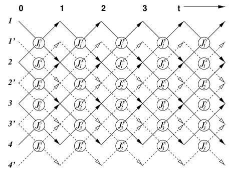
FIG. 1.: Sketch of the directed walk problem corresponding to the transfer matrix given in eq. (18). Note that one has two independent walks in the ${\bf t}$-direction of the diagonally layered square lattice, corresponding to the independent subspaces for the eigenvalue problem (see text). The coupling strength $J_{i}^{x,y}$ are the transition rates for the random walker from one sites in row $i$ to those in row $i\pm 1$.

C Local order-parameters

Next we are going to study the long-range-order in the ground state of the system. Having free boundary conditions, as in (2), the expectation value of the local spin operator $\langle 0|S_{l}^{x}|0\rangle$ (and $\langle 0|S_{l}^{y}|0\rangle$) is zero for finite chains. Then the scaling behavior of the spin operator can be obtained from the asymptotic behavior of the (imaginary) time-time correlation function:

$$G_{l}^{x}(\tau) = \langle 0|S_{l}^{x}(\tau)S_{l}^{x}(0)|0\rangle$$ (21)

$$= \sum_{\langle n|}|\langle n|S_{l}^{x}|0\rangle|^{2}\exp[-\tau(E_{n}-E_{0})]\;,$$ (22)

where $|0\rangle$ and $|n\rangle$ denote the ground state and the $n$th excited state of $H$ in Eq. (2), with energies $E_{0}$ and $E_{n}$, respectively. In the phase with long-range-order the first excited state is asymptotically degenerate with the ground state in the thermodynamic limit, thus the sum in Eq. (22) is dominated by the first term. In the large $\tau$ limit $\lim_{\tau\to\infty}G_{l}^{x}(\tau)=(m_{l}^{x})^{2}$, thus the local order-parameter is given by the off-diagonal matrix element:

$$m_{l}^{x}=\langle 1|S_{l}^{x}|0\rangle\;.$$ (23)

In the free fermion representation $S_{l}^{x}$ is expressed as[28]

$$S_{l}^{x}={1\over 2}A_{1}B_{1}A_{2}B_{2}\dots A_{l-1}B_{l-1}A_{l}\;$$ (24)

with

$$\begin{array}[]{lcl}A_{i}&=&\sum_{q=1}^{L}\Phi_{q}(i)(\eta_{q}^{+}+\eta_{q})\;,\\ B_{i}&=&\sum_{q=1}^{L}\Psi_{q}(i)(\eta_{q}^{+}-\eta_{q})\;.\end{array}$$ (25)

Using $|1\rangle=\eta_{1}^{+}|0\rangle$ the matrix-element in Eq. (23) is evaluated by Wick’s theorem. Since for $i\neq j~{}~{}\langle 0|A_{i}A_{j}|0\rangle=\langle 0|B_{i}B_{j}|0\rangle=0$ we obtain for the local order-parameter:

$$m_{l}^{x}={1\over 2}\left|\,\matrix{H_{1}&G_{11}&G_{12}&\ldots&G_{1l-1}\cr H_{2}&G_{21}&G_{22}&\ldots&G_{2l-1}\cr\vdots&\vdots&\vdots&\ddots&\vdots\cr H_{l}&G_{l1}&G_{l2}&\ldots&G_{ll-1}\cr}\right|\;,$$ (26)

where

$$H_{j} = \langle 0|\eta_{1}A_{j}|0\rangle=\Phi_{1}(j)$$ (27)

$$G_{jk} = \langle 0|B_{k}A_{j}|0\rangle=-\sum_{q}\Psi_{q}(k)\Phi_{q}(j)\;.$$ (28)

For surface spins the local order-parameter is simply given by $m_{1}^{x}=\Phi_{1}(1)/2$, which can be evaluated in the thermodynamic limit $L\to\infty$ in the phase with long-range-order, when $\epsilon_{1}=0$. Using the normalization condition $\sum_{l}|\Phi_{1}(l)|^{2}=1$ we obtain for the surface order parameter:

$$\begin{array}[]{lcll}m_{1}^{x}&=&\displaystyle{1\over 2}\left[1+\sum_{l=1}^{L/2-1}\prod_{j=1}^{l}\left(J^{y}_{2j-1}\over J^{x}_{2j}\right)^{2}\right]^{-1/2}&\quad XY\\ m_{1}^{x}&=&\displaystyle{1\over 2}\left[1+\sum_{l=1}^{L/2-1}\prod_{j=1}^{l}\left(J_{2j-1}\over J_{2j}\right)^{2}\right]^{-1/2}&\quad XX.\end{array}$$ (29)

We note that this formula is exact for finite chains if we use fixed spin boundary condition, $S_{L}^{x}=\pm 1/2$, wich amounts to have $J_{L-1}^{y}=0$. In the fermionic description the two-fold degeneracy of the energy levels, corresponding to $S_{L}^{x}=1/2$ and $S_{L}^{x}=-1/2$, is manifested by a zero energy mode in Eq. (13) and from the corresponding eigenvector one obtains $m_{1}^{x}$ in Eq. (29) for any finite chain.

For non-surface spins the expression of the local order-parameter in Eq. (26) can be simplified by using the relations in (19). Then, half of the elements of the determinant in (26) are zero, the non-zero-elements being arranged in a checker-board pattern, and $m_{l}^{x}$ can be expressed as a product of two determinants of half-size, which reads for $l=2j$ as:

$$m_{2j}^{x}= \displaystyle{1\over 2} \left|\,\matrix{H_{1}&G_{1,2}&G_{1,4}&\ldots&G_{1,2j-2}\cr H_{3}&G_{3,2}&G_{3,4}&\ldots&G_{3,2j-2}\cr\vdots&\vdots&\vdots&\ddots&\vdots\cr H_{2j-1}&G_{2j-1,2}&G_{2j-1,4}&\ldots&G_{2j-1,2j-2}\cr}\right|$$ (30)

$$\times \left|\,\matrix{G_{2,1}&G_{2,3}&\ldots&G_{2,2j-1}\cr G_{4,1}&G_{4,3}&\ldots&G_{4,2j-1}\cr\vdots&\vdots&\ddots&\vdots\cr G_{2j,1}&G_{2j,3}&\ldots&G_{2j,2j-1}\cr}\right|\;.$$ (31)

The local order-parameter $m_{l}^{y}$, related to the off-diagonal matrix-element of the operator $S_{l}^{y}$ can be obtained from Eqs. (26) and (29) by exchanging $J_{l}^{x}\leftrightarrow J_{l}^{y}$.

For the $S^{z}_{l}$ operator the autocorrelation function, $G^{z}_{l}(\tau)$, can be expressed in a similar way as $G^{x}_{l}(\tau)$ in Eq. (22) and its long time limit, $\lim_{\tau\to\infty}G_{l}^{z}(\tau)=(m_{l}^{z})^{2}$, is given by the local order parameter

$$m_{l}^{z}=\langle\phi_{z}|S_{l}^{z}|0\rangle\;.$$ (32)

Here $|\phi_{z}\rangle$ denotes the lowest eigenstate of $H$ in Eq. (2) having a non-vanishing matrix-element of $S_{l}^{z}$ with the ground state. In the free fermion representation $S_{l}^{z}$ can be written as[28]

$$S_{l}^{z}={1\over 2}A_{l}B_{l}\;$$ (33)

and the off-diagonal order-parameter is given by:

$$m_{l}^{z}={1\over 2}|-\Phi_{1}(l)\Psi_{2}(l)+\Psi_{1}(l)\Phi_{2}(l)|\;.$$ (34)

For the $XX$ model one can obtain simple expressions using the relations in Eqs. (20) as:

$$m_{2i-1}^{z} =\frac{1}{2}[\Phi_{1}(2i-1)]^{2}\;,$$ (36)

$$\quad XX{\rm-model}$$

$$m_{2i}^{z} =\frac{1}{2}[\Psi_{1}(2i)]^{2}\;.$$ (37)

D Autocorrelations

Next we consider the dynamical correlations of the system as a function of the imaginary time $\tau$. First, we note that the correlations between $x$-components of the surface spins can be obtained directly from eq(22) as:

$$G_{1}^{x}(\tau) = {1\over 4}\sum_{q}|\Phi_{q}(1)|^{2}\exp(-\tau\epsilon_{q})$$ (38)

$$= {1\over 4}\sum_{i}^{L/2}|\Phi_{2i-1}(1)|^{2}\exp(-\tau\epsilon_{2i-1})\;,$$ (39)

where we have used the relations in Eq. (19).

For bulk spins the matrix-element $\langle n|S_{l}^{x}|0\rangle$ in eq(22) is more complicated to evaluate, one has to go back to the first equation of (22) and considers the time-evolution in the Heisenberg picture:

$$S_{l}^{x}(\tau) = \exp(\tau H)S_{l}^{x}\exp(-\tau H)$$ (40)

$$= {1\over 2}A_{1}(\tau)B_{1}(\tau)\dots A_{l-1}(\tau)B_{l-1}(\tau)A_{l}(\tau)\;.$$ (41)

The general time and position dependent correlation function

$$\langle S_{l}^{x}(\tau)S_{l+n}^{x}\rangle={1\over 4}\langle A_{1}(\tau)B_{1}(\tau)\cdots A_{l}(\tau)A_{1}B_{1}\dots A_{l+n}\rangle\;,$$ (42)

can then be expanded using Wick’s theorem into a sum over products of two-operator expectation values, which can be expressed in a compact form as a Pfaffian:

  

$$4\langle S_{l}^{x}(\tau)S_{l+n}^{x}\rangle = \left.\matrix{|\;\langle A_{1}(\tau)B_{1}(\tau)\rangle&\langle A_{1}(\tau)A_{2}(\tau)\rangle&\langle A_{1}(\tau)B_{2}(\tau)\rangle&\cdots\quad\langle A_{1}(\tau)A_{l}(\tau)\rangle&\langle A_{1}(\tau)A_{1}\rangle&\cdots\quad\langle A_{1}(\tau)A_{l+n}\rangle\cr&\langle B_{1}(\tau)A_{2}(\tau)\rangle&\langle B_{1}(\tau)B_{2}(\tau)\rangle&\cdots\quad\langle B_{1}(\tau)A_{l}(\tau)\rangle&\langle B_{1}(\tau)A_{1}\rangle&\cdots\quad\langle B_{1}(\tau)A_{l+n}\rangle\cr&&\langle A_{2}(\tau)B_{2}(\tau)\rangle&\cdots\quad\langle A_{2}(\tau)A_{l}(\tau)\rangle&\langle A_{2}(\tau)A_{1}\rangle&\cdots\quad\langle A_{2}(\tau)A_{l+n}\rangle\cr&&&\ddots&&\vdots\cr&&&&&\langle B_{l+n-1}A_{l+n}\rangle}\right|$$ (43)

$$= \pm\left[{\rm det}\,C_{ij}\right]^{1/2}\;,$$ (44)

where $C_{ij}$ is an antisymmetric matrix $C_{ij}=-C_{ji}$, with the elements of the Pfaffian (44) above the diagonal. At zero temperature the elements of the Pfaffian are the following:

$$\langle A_{j}(\tau)A_{k}\rangle = \sum_{q}\Phi_{q}(j)\Phi_{q}(k)\exp(-\tau\epsilon_{q})\;,$$ (45)

$$\langle A_{j}(\tau)B_{k}\rangle = \sum_{q}\Phi_{q}(j)\Psi_{q}(k)\exp(-\tau\epsilon_{q})\;,$$ (46)

$$\langle B_{j}(\tau)B_{k}\rangle = -\sum_{q}\Psi_{q}(j)\Psi_{q}(k)\exp(-\tau\epsilon_{q})\;,$$ (47)

$$\langle B_{j}(\tau)A_{k}\rangle = -\sum_{q}\Psi_{q}(j)\Phi_{q}(k)\exp(-\tau\epsilon_{q})\;,$$ (48)

whereas the equal-time contractions are given below (25). For the finite temperature contractions see c.f. [30].

For longitudinal correlations the matrix-elements of $S_{l}^{z}$ in (33) is given in a simple form for any position, $l$, therefore $G_{l}^{z}(\tau)$ can be obtained from the analogous expression to (22) as

$$G_{l}^{z}(\tau)={1\over 4}\sum_{q}\sum_{p>q} |-\Psi_{p}(l)\Phi_{q}(l)+\Psi_{q}(l)\Phi_{p}(l)|^{2}$$ (49)

$$\cdot \exp[-\tau(\epsilon_{q}+\epsilon_{p})]\;.$$ (50)

III Phenomenological theory from scaling of rare events

In classical random ferromagnets where the critical behavior is controlled by a random fixed point the distribution of several physical quantities (order-parameters, correlations, autocorrelations, etc.) is broad and as a consequence these quantities are not self-averaging: their average and most-probable or typical values are different. In random quantum spin chains the critical properties are expected to be controlled by the infinite-randomness critical fixed point[31], where the distributions are extremely (logarithmically) broad and as a consequence the average and typical behavior of these quantities are completely different. The average is dominated by such realizations (the so called rare events), which have a very large contribution, but their fraction is vanishing in the thermodynamic limit. In this Section we identify these rare events for the random $XY$ (and $XX$) model and use their properties to develop a phenomenological theory. Our basic observations are related to exact relations about the surface order-parameter and the energy of low-lying excitations.

A Surface order-parameter and the mapping to adsorbing random walks

The local order-parameter at the boundary is given by the simple formula in Eq. (29) as a sum of products of the ratio of the couplings $J^{y}_{2j-1}$ and $J^{x}_{2j}$. It is easy to see from Eq. (29) that in the thermodynamic limit the average surface order-parameter is zero (non-zero), if the geometrical mean of the $J^{x}_{2j}$ couplings is (smaller) grater than that of the $J^{y}_{2j-1}$ couplings. From this the definition of the control parameters in Eqs. (3) and (6) follows.

Next we compute the average value of the surface order-parameter for the extreme binary distribution, i.e. the limit $\lambda\to 0$ [32] in (8). For a random realization of the couplings the surface order-parameter at the critical point ($p=q=1/2$) is zero, whenever a product of the form of $\prod_{i=1}^{l}(J_{i}^{x})^{-2}$, $l=1,2,\dots,L$ is infinite, i.e. the number of $\lambda$-couplings exceeds the number of $\lambda^{-1}$-couplings in any of the $[1,l]$ intervals. Otherwise the surface order-parameter has a finite value of $O(1)$. The distribution of the couplings $J^{x}$ can be represented by one-dimensional random walks that start at zero and make the $i$-th step upwards (for $J^{x}_{2i}=\lambda^{-1}$) or downwards (for $J^{x}_{2i}=\lambda$). The ratio of walks representing a sample with finite surface order-parameter is given by the survival probability of the walk $P_{surv}$, i.e. the probability of the walker to stay always above the starting point in $L/2$ steps which is given by $P_{surv}(L/2)\sim L^{-1/2}$.

Next we consider the vicinity of the critical point, when the scaling behavior of the average surface order-parameter can be obtained from the survival probabilities of biased random walks[15], where the probability that the walker makes a step towards the adsorbing boundary, $q$, is different from that of a step off the boundary, $p$. The control parameter of the walk, $\delta_{w}=p-q$, is analogous to the quantum control parameters $\delta_{a}$ and $\delta_{d}$ in Eqs. (3) and (6), respectively. Thus we have the basic correspondences between the average surface order-parameter of the $XY$ (and $XX$) model and the surviving probability of adsorbing random walks:

$$[m_{1}(\delta,L)]_{av}\sim P_{\rm surv}(\delta_{w},L/2),~{}~{}~{}\delta\sim\delta_{w}\;,$$ (51)

We recall the asymptotic properties of the surviving probability of adsorbing random walks[15]. For unbiased walks:

$$P_{\rm surv}(\delta_{w}=0,L)\sim L^{-1/2}\;,$$ (52)

for walks with a drift away from the wall:

$$P_{\rm surv}(\delta_{w}>0,L\to\infty)\sim\delta_{w}\;,$$ (53)

and for walks with a drift towards the wall:

$$P_{\rm surv}(\delta_{w}<0,L)\sim\exp(-L/\xi_{w}),~{}~{}~{}\xi_{w}\sim\delta_{w}^{-2}\;.$$ (54)

In this way we have identified the rare events for the surface order-parameter, which are samples with a coupling distribution which have a surviving walk character. The scaling properties of the average surface order-parameter and the correlation length immediately follow from Eqs. (52), (53) and (54) and will be evaluated in Section IV.A.

B Scaling of low-energy excitations

The rare events controlling the surface order-parameter are also important for the low-energy excitations. Our results are obtained by using a simple relation for the smallest gap, $\epsilon_{1}(l)$, of an open system of size $l$, i.e. with free boundary conditions, expecting that it goes to zero at least as $\sim 1/l$. With this condition one can neglect the r.h.s. of the eigenvalue problem of ${\bf T}$ in Eq. (18), ${\bf T}V_{1}=\epsilon_{1}V_{1}$, and derive approximate expressions for the eigenfunctions $\Phi_{1}$ and $\Psi_{1}$. With these one arrives at:

$$\epsilon_{1}(l)\sim m_{1}^{x}m_{l-1}^{x}J^{y}_{l-1}\prod_{j=1}^{l/2-1}{J^{y}_{2j-1}\over J^{x}_{2j}}\;,$$ (55)

Here $m_{1}^{x}$ is defined in (29) and the surface order-parameter at the other end of the chain, $m_{l-1}^{x}$, is given as in Eq. (29) replacing $J^{y}_{2j-1}/J^{x}_{2j}$ by $J^{y}_{l+1-2j}/J^{x}_{l-2j}$. (For details of the derivation of a similar expression for the quantum Ising chain see in Ref.[33].)

Before using the relation in Eq. (55) we note that (surface) order and the presence of low-energy excitations are inherently related. These samples with an exponentially (in the system size) small gap have finite, $O(1)$, order-parameters at both boundaries and the coupling distribution follows a surviving walk picture. Such type of coupling configuration represents a strongly coupled domain (SCD), which at the critical point extends over the size of the system, $L$. In the off-critical situation, in the Griffiths phase the SCD-s have a smaller extent, $l\ll L$, and they are localized both in the volume and near the surface of the system. The characteristic excitation energy of an SCD can be estimated from Eq. (55) as

$$\epsilon_{1}(l)\sim\prod_{j=1}^{l/2-1}{J^{y}_{2j-1}\over J^{x}_{2j}}\sim\exp\Bigl{\{}-\frac{l_{\rm tr}}{2}\overline{\ln(J^{y}/J^{x})}\Bigr{\}}\;,$$ (56)

where $l_{\rm tr}$ measures the size of transverse fluctuations of a surviving walk of length $l$ and $\overline{\ln(J^{x}/J^{y})}$ is an average ratio of the couplings, (it is $\overline{\ln(J^{e}/J^{o})}$ for the $XX$ model).

At the critical point ($\delta=0$), where $l\sim L$, the size of transverse fluctuations of the couplings in the SCD is $l_{\rm tr}\sim L^{1/2}$[15]. Consequently we obtain from Eq. (56) for the scaling relation of the gap:

$$\epsilon(\delta=0,L)\sim\exp(-{\rm const}\cdot L^{1/2})\;.$$ (57)

Then the appropriate scaling variable is $\ln\epsilon/\sqrt{L}$ and the distribution of the excitation energy is extremely (logarithmically) broad.

In the Griffiths phase the size of a SCD can be estimated along the lines of Ref.[15] as $l\sim\xi_{w}\ln L$ and the size of transverse fluctuations is now $l_{\rm tr}\sim l\sim\ln L$. Setting this estimate into Eq. (56) we obtain for the scaling relation of the gap:

$$\epsilon(L)\sim L^{-z}\;,$$ (58)

where $z$ is the dynamical exponent as defined in Eq. (1). The distribution of low-energy excitations can be obtained from the observation that an SCD can be localized at any site of the chain, thus $P_{L}(l)\sim P_{L}(\ln\epsilon)\sim L$. For a given large $L$ the scaling combination from Eq. (58) is $L\epsilon^{1/z}$, thus we have:

$$P(\epsilon)\sim\epsilon^{-1+1/z}\;.$$ (59)

As already mentioned $z$ is a continuous function of the quantum control parameter $\delta$ and we are going to calculate its exact value in Section V.

C Scaling theory of correlations

The scaling behavior of critical average correlations is also inherently connected to the properties of rare events. Here the quantity of interest is the probability $P^{\mu}(l)$, which measures the fraction of rare events of the local order-parameter $m_{l}^{\mu}$. For the surface order-parameter $m_{1}^{x}$ it is given by the surviving probability, $P^{x}(1)=P_{surv}$, according to Eq. (51). We start with the equal-time correlations in Eq. (4). In a given sample there should be local order at both reference points of the correlation function in order to have $C^{\mu}(r)=O(1)$. This is equivalent of having two SCD-s in the sample which occur with a probability of $P_{2}^{\mu}(l,l+r)$, which factorizes for large separation $\lim_{r\to\infty}P_{2}^{\mu}(l,l+r)=P^{\mu}(l)P^{\mu}(L+r)$, since the disorder is uncorrelated. The probability of the occurrence of a SCD at position $l$, $P^{\mu}(l)$, has the same scaling behavior as the local order-parameter $[m^{\mu}_{l}]_{\rm av}=[\langle\phi_{\mu}|S^{\mu}_{l}|0\rangle]_{\rm av}$, which behaves at a bulk point, $0<l/L<1$, as:

$$[m^{\mu}_{l}(L)]_{\rm av}\sim L^{-x^{\mu}}\;,$$ (60)

whereas for a boundary point, $l=1$, this relation involves the surface scaling dimension $x^{\mu}_{1}$. Consequently $P^{\mu}(l)$ transforms as $P^{\mu}(l/b)=b^{-x^{\mu}}P^{\mu}(l)$ under a scaling transformation, when lengths are rescaled by a factor $b>1$. Recalling that for spatial correlations there should be two independent SCD-s we obtain the transformation law:

$$[C^{\mu}(r)]_{\rm av}=b^{-2x^{\mu}}[C^{\mu}(r/b)]_{\rm av}\;.$$ (61)

Now taking $b=r$ one recovers the power-law decay in Eq. (5) with the exponent

$$\eta^{\mu}=2x^{\mu}\;.$$ (62)

For critical time-dependent correlations the scaling behavior is different from that in Eq. (61). This is due to the fact that disorder in the time direction is perfectly correlated and the autocorrelation function in a given sample is $G^{\mu}_{l}(\tau)=O(1)$, if there is one SCD localised at position $l$. Therefore the average autocorrelation function $[G^{\mu}_{l}(\ln\tau)]_{\rm av}$ scales as the probability of rare events $P^{\mu}(l)$:

$$[G^{\mu}_{l}(\ln\tau)]_{\rm av}=b^{-x^{\mu}}[G^{\mu}_{l}(\ln\tau/b^{1/2})]_{\rm av}\;,$$ (63)

where we have used the relation in Eq. (70) between relevant length and time at the critical point. Taking the length scale as $b=(\ln\tau)^{2}$ we obtain for points $l$ in the volume:

$$[G^{\mu}_{l}(\tau)]_{\rm av}\sim(\ln\tau)^{-\eta^{\mu}}\;,$$ (64)

whereas for surface spins, $l=1$, one should use the corresponding surface decay exponent $\eta^{\mu}_{1}$.

Next we turn to study the scaling properties of the average correlation functions in the Griffiths phase, i.e. outside the critical point. For equal-time correlations in a sample $C^{\mu}(r)=O(1)$, if the SCD extends over a large distance of $r$, which according to Eq. (54) is exponentially improbable. Thus the average spatial correlations decay as

$$[C^{\mu}(r)]_{\rm av}\sim\exp(-r/\xi),~{}~{}~{}\xi\sim\xi_{w}\;,$$ (65)

where $\xi_{w}$ is defined in Eq. (54). On the other hand the autocorrelation function in a sample is $G^{\mu}(\tau)=O(1)$, if there is one SCD localized at $l$, which occurs with a probability of $P^{\mu}(l)\sim 1/L$. Consequently the average autocorrelation function, which scales as $P^{\mu}(l)$, transforms under a scaling transformation as:

$$[G^{\mu}_{l}(\tau)]_{\rm av}=b^{-1}[G^{\mu}_{l/b}(\tau/b^{z})]_{\rm av}~{}~{}~{}\delta>0\;,$$ (66)

where we used the scaling combination $\tau/b^{z}$ in accordance with Eq. (1). Now taking $b=\tau^{1/z}$ we obtain

$$[G^{\mu}_{l}(\tau)]_{\rm av}\sim\tau^{-1/z}\;,$$ (67)

for any type of autocorrelations, both in the volume and at the surface.

IV Critical properties

Here we consider in detail the random $XY$ and $XX$ chains in the vicinity of the critical points, as defined in Eqs. (3) and (6), respectively. The off-critical properties of the systems in the Griffiths phase are presented afterwards in the following Section.

A Length- and time-scales

As we argued in the previous Chapter the average behavior of random quantum spin chains are inherently related to the properties of the rare events, which are SCD-s, having a coupling distribution of surviving RW character. The typical size of an SCD, as given by $\xi_{w}$ in Eq. (54), is related to the average correlation length of the system, $[\xi]_{\rm av}$. Then using the correspondences in Eqs. (51), (54) and (65) we get the relation:

$$[\xi]_{\rm av}\sim|\delta|^{-\nu},~{}~{}~{}\nu=2\;.$$ (68)

The typical correlation length, $\xi_{\rm typ}$, as measured by the average of the logarithm of the correlation function is different from the average correlation length. One can estimate the typical value by studying the formula in Eq. (29) for the surface order-parameter, where the products are typically of $\prod_{j}(J^{y}_{2j-1}/J^{x}_{2j})^{2}\sim\exp({\rm const}\cdot|\delta|L)$, thus $[m_{s}(L,\delta\langle 0)]_{\rm typ}\sim\exp(-{\rm const}\cdot|\delta|L)\sim\exp(-L/\xi_{\rm typ})$. Thus we obtain:

$$\nu_{\rm typ}=1\;.$$ (69)

We note that at the critical point the largest value of the above products is typically of $\prod_{j}(J^{y}_{2j-1}/J^{x}_{2j})^{2}\sim\exp(AL^{1/2})$, since the transverse fluctuations in the couplings are of $O(L^{1/2})$, thus we have $[m_{s}(L,\delta=0)]_{\rm typ}\sim\exp(-{\rm const}\cdot L^{1/2})$.

As shown in Eq. (56) the value of the smallest gap is related to the size of transverse fluctuations of an SCD, $l_{\rm tr}$. Away from the critical point, when the correlation length is finite, one has $l_{\rm tr}\sim\xi^{1/2}$, and therefore the typical relaxation time of a sample with typical correlation length $\xi$ scales as

$$\ln t_{r}\sim\xi^{1/2}\;.$$ (70)

We note that the results in this part about length- and time-scales are valid both for the $XY$ and $XX$ models. They also hold in identical form for the random TIM[9, 15], which can be understood as a consequence of the mapping of the $XY$-chain into decoupled TIM-s. (See Appendix.) Since the corresponding scaling expressions for the random TIM have been studied in detail in previous numerical work[13, 15] we do not repeat these calculations here.

B Quasi-long-range-order

At the critical point of random quantum chains the equal-time correlations decay with a power-law, (see Eq. (5)), thus there is QLRO in the system. The decay exponent of critical correlations are related to the scaling exponent $x^{\mu}$ of the fraction of rare events of the given quantity (see Eq. (62)) and its value generally depends on the type of correlations of the disorder, thus it could be different for the $XY$ and the $XX$ models. Analyzing the scaling properties of the rare events in the $XY$ and $XX$ chains we have calculated the critical decay exponents of different correlation functions, both between two spins in the volume and for end-to-end correlations. Our results are presented in Table I.

	$\eta^{x}(XY)$	$\eta^{x}(XX)$	$\eta^{z}(XY)$	$\eta^{z}(XX)$
bulk	$3-\sqrt{5}^{(**)}$	$2^{(*)}$	$4$	$2^{(*)}$
surface	$1$	$1$	$2$	$1$

TABLE I: Decay exponents of critical correlations in the random $XY$ and $XX$ chains. The exponents with a superscript ^(∗) are those calculated by Fisher with the RG method[4], whereas ^(∗∗) follows from the results of the random TIM in Ref.[9].

In the following we are going to derive these exponents by analytical and scaling methods and then confront them with the results of numerical calculations.

1 Longitudinal order-parameter

We start with the scaling behavior of the longitudinal order-parameter $m_{l}^{z}$, which in the $XX$ chain is given by the simple formula in Eq. (36). Summing over all sites one gets the sum-rule

$$\sum_{l=1}^{L}m_{l}^{z}=1~{}~{}~{}{\rm XX-model}\;,$$ (71)

where we have used Eq. (19) and the fact that the $\Phi_{q}$ and $\Psi_{q}$ are normalized. Since this sum-rule is valid for the average quantities, too, we get immediately

$$[m^{z}_{l}]_{\rm av}=L^{-1}\tilde{m}^{z}(l/L)\;,$$ (72)

where $\tilde{m}^{z}(\tilde{l})$ is a scaling function with $\tilde{l}=l/L$. Consequently for bulk spins the finite-size dependence of the local order-parameter is $[m^{z}_{l}]_{\rm av}\sim L^{-1}$, thus from Eq. (60) we have $x^{z}(XX)=1$ and from Eq. (62) the decay exponent is

$$\eta^{z}(XX)=2$$

as given in Table I. A further consequence of the sum-rule in Eq. (71) is that the average value of the bulk order-parameter is the same, if the averaging is performed over any single sample. Thus the order-parameter $m^{z}$ and the correlation function $\langle S^{z}_{l}S^{z}_{l+r}\rangle$ are self-averaging. This is quite special in disordered systems where the correlations are generally not self-averaging[34]. The self-averaging properties of the $S^{z}$-correlations provides an explanation of the accurate numerical determination of the decay exponent $\eta^{z}(XX)=2$ in previous numerical work[25, 26].

The surface order-parameter $m_{1}^{z}$ for the $XX$ model satisfies the relation $m_{1}^{z}=2\left(m_{1}^{x}\right)^{2}$, which follows from Eqs. (29) and (36). Then a rare event with $m_{1}^{x}=O(1)$ is also a rare event for the order-parameter $m_{1}^{z}$, consequently the fraction of rare-events $P^{z}_{1}$ is given by the surviving probability in Eq. (52). Thus the scaling dimension is $x^{z}_{1}=1/2$ and the decay exponent of critical end-to-end correlations is

$$\eta^{z}_{1}(XX)=1$$

as shown in Table I.

We studied the order-parameter profile $[m_{l}^{z}]_{\rm av}$ numerically for large finite systems up to $L=256$. As shown in Fig. 2 the numerical points of the scaled variable $L[m^{z}_{l}]_{\rm av}$ are on one scaling curve $\tilde{m}^{z}(\tilde{l})$ for different values of $L$. The scaling curve has two symmetric branches for odd and even lattice sites, which cross at $l=L/2$. The upper part of the curves in the large $L$ limit is very well described by the function $\tilde{m}^{z}(\tilde{l})_{\rm u}={\cal A}\sin(\pi\tilde{l})^{-1/2}$, which corresponds to the conformal result about off-diagonal matrix-element profiles[27]:

$$[m_{l}^{\mu}]_{\rm av}\sim\left({\pi\over L}\right)^{x^{\mu}}\left(\sin\pi{l\over L}\right)^{x^{\mu}_{1}-x^{\mu}}\;,$$ (73)

with $x^{z}=1$ and $x^{z}_{1}=1/2$. On the other hand the lower part of the curves in Fig. 2 is given by $\tilde{m}^{z}(\tilde{l})_{\rm l}={\cal A}\sin(\pi\tilde{l})$, which corresponds to Eq. (73) with $x^{z}_{2}=2$. Thus we obtain that average critical correlations between two spins which are next to the surface are decaying as $[C^{z}(2,L-1)]_{\rm av}\sim L^{-4}$. Using the sum-rule for the profile in Eq. (71) and the conformal predictions one can determine the pre-factor $\cal{A}$ from normalization. Then from the equation ${\cal A}/2\int_{0}^{1}[(\sin\pi x)^{-1/2}+\sin\pi x]dx=1$, one gets ${\cal A}=.86735$, which fits well the numerical data on Fig. 2.

FIG. 2.: Finite size scaling plot of the longitudinal order-parameter profiles $[m_{l}^{z}]_{\rm av}$ for the $XX$ model at criticality for different system sizes calculated numerically with the fermion method using eq. (36). The data are for the uniform distribution, averaged over 50000 samples. The conformal results are indicated by full lines.

These results about the conformal properties of the profile are in agreement with similar studies of the random TIM[14, 15]. Thus it seems to be a general trend that critical order-parameter profiles of random quantum spin chains are described by the results of conformal invariance, although these systems are strongly anisotropic (see Eq. (70)) and therefore not conformally invariant.

Next we turn to study the order-parameter $m_{l}^{z}$ and the longitudinal correlation function in the random $XY$ model. In this model the disorder in the $J^{x}_{l}$ and $J^{y}_{l}$ couplings is uncorrelated, therefore one can perform averaging in the two subspaces $T_{\sigma}$ and $T_{\tau}$, or in the two decoupled TIM-s, independently. Note that the expression for $m_{l}^{z}$ in Eq. (34) is given as a product of two vector-components, where each vector belongs to different subspaces and have the same average behavior. Since the couplings entering the two separate eigenvalue problems are independent one gets for the disorder average

$$[m_{l}^{z}]_{\rm av}=[\Phi_{1}(l)]_{\rm av}\cdot[\Psi_{2}(l)]_{\rm av}\;.$$ (74)

Since the probability for $m_{l}^{z}$ being of order one is the product of the probabilities for $\Phi_{1}(l)$ and $\Psi_{2}(l)$ being of order one we conclude that the scaling dimension for $m_{l}^{z}$ in the random $XY$ chain is twice that for the random $XX$ chain. Thus the decay exponents are

$$\eta^{z}(XY)=4$$

and

$$\eta^{z}_{1}(XY)=2$$

in the bulk and at the surface, respectively, as shown in Table I.

The numerical results about the order parameter profile is shown in Fig. 3. The data collapse is satisfactory, although not as good as for the $XX$ model. Similar conclusion holds for the relation with the conformally predicted profile, which is also presented in Fig. 3.

FIG. 3.: Finite size scaling plot of the longitudinal order-parameter profiles $[m_{l}^{z}]_{\rm av}$ for the $XY$ model at criticality for different system sizes calculated numerically with the fermion method using eq. (36). The data are for the uniform distribution, averaged over 50000 samples.

2 Transverse order-parameter

We start with the surface order-parameter, $m_{1}^{x}$, as given by the simple formula in Eq. (29). This formula is identical both for the $XY$ and $XX$ models and its average behavior follows from the adsorbing random walk mapping in Section III.A. Then from Eqs. (51) and (52) one gets $x^{x}_{1}=1/2$ and

$$\eta^{x}_{1}=1\;,$$

both for the random $XY$ and $XX$ models, as shown in Table I. The value of the decay exponents follows also from the mapping to two TIM-s. As shown in Eq. (106) in the Appendix the correlation function $\langle S_{2l}^{x}S_{2l+2r}^{x}\rangle$ is expressed as the product of spin correlations in the two TIM’s, one with open boundary conditions, but the other is taken with fixed-spin boundary conditions in terms of dual variables. For end-to-end correlations this second factor in the product is unity, since it is the correlation between two fixed spins. Therefore end-to-end correlations between the random TIM and the random $XY$ and $XX$ models are identical and the decay exponent corresponds to the value in Table I.

FIG. 4.: Transverse order-parameter profile $[m_{l}^{x}]_{\rm av}$ for the $XY$ model at criticality for different system sizes calculated numerically with the fermion method using eq. (31). The data are for the uniform distribution, averaged over 50000 samples.

For bulk correlations one can easily find the answer for the $XY$ model with the mapping in Eq. (106). When the two points of reference are located far from the boundary the boundary condition does not matter and after performing the independent averaging for the two factors of the product one obtains $[\langle S_{2l}^{x}S_{2l+2r}^{x}\rangle]_{\rm av}=1/4[\langle\sigma^{x}_{l}\sigma^{x}_{l+r}\rangle]_{\rm av}^{2}$, thus

$$\eta^{x}(XY)=2\eta(TIM)=3-\sqrt{5}\;,$$ (75)

where the last result follows from Fisher’s RG calculation[9]. (As shown in Ref.[35] the rare events for the bulk order-parameter in the TIM are samples having a coupling distribution of average persistence character). The scaling exponent $x^{x}(XY)$ can identically be obtained from the expression of the order-parameter profile in Eq. (31), which is in the form of a product of the two Ising order-parameters and for the $XY$ model the two factors are averaged independently.

For the $XY$ model the numerically calculated profile is shown in Fig. 4. The scaling plot with the exponents in Table I is reasonable, although larger systems and even more samples would be needed to reach the expected asymptotic behavior, as predicted by conformal invariance in Eq. (73).

The arguments leading to the prediction (75) for the transverse bulk order parameter exponent do not apply for the $XX$ model and one cannot obtain a simple estimate for the bulk decay exponent from Eqs. (106) or (31) due to the following reason. The expressions with the parameters of the two quantum Ising chains contain real and dual variables for the two ($\sigma$ and $\tau$) systems. Since $J^{x}_{l}=J^{y}_{l}=J_{l}$ a domain of strong couplings in the $\sigma$ chain corresponds to a domain of weak couplings in the $\tau$ chain and reverse. Therefore the rare events of the TIM can not be simply related to the rare-events of the $XX$ chain.

The value for $\eta^{x}(XX)$, however, can be obtained by the following argument. For simplicity let us consider the extreme binary distribution in which $J_{2i}=1$ and $J_{2i-1}=\lambda$ or $1/\lambda$ with probability $1/2$, taking the limit $\lambda\to 0$. Then, from Eq.(29), one gets only then a non-vanishing transversal surface magnetization, when the disorder configuration has a surviving walk character (meaning $\prod_{i=1}^{l}J_{2i-1}<\infty$ for all $l=1,\ldots,L/2-1$). This implies, also for general distributions of couplings that $m_{1}^{x}\sim{\cal O}(1)$ only if the surface spin is weakly coupled to the rest of the system. It is instructive to note the difference to the surface magnetization in the TIM, where $m_{1}^{x}\sim{\cal O}(1)$ when the surface spin is strongly coupled to the rest of the system, meaning that $\prod_{i=1}^{l}(1/J_{i})<\infty$ for all $l=1,\ldots,L-1$ for the extreme binary distribution.

The same remains true for a bulk spin, which also has non-vanishing transverse magnetization only if it is weakly coupled to the rest of the system (the trivial example being when both its couplings to the left and to the right are exactly zero, which gives the maximum value $m_{1}^{x}=1/2$). Thus the central spin in a chain of length, say $2L-1$, has $m^{x}\sim{\cal O}(1)$ if and only if the bond-configurations on both sides have surviving character, as it is depicted in fig. 4 for the extreme binary distribution. Since the probability $P_{surv}(L/2)$ for a configuration of $L/2$ couplings to represent a surviving walk is $P_{surv}(L/2)\sim L^{-1/2}$ it is

$$m_{l}^{x}\sim\{P_{surv}(L/2)\}^{2}\sim L^{-1},\quad{\rm i.e.}\quad x^{x}(XX)=1\;.$$ (76)

From this one obtains

$$\eta^{x}(XX)=2\;,$$ (77)

as given in Table I.

FIG. 5.: Sketch of a bond configuration for a chain of length $2L-1$ that gives a non-vanishing transverse magnetization $m^{x}\sim{\cal O}(1)$ for the central (bulk) spin. The example is for the extreme binary distribution. Weak couplings ($J_{2i-1}=\lambda$) correspond to downward steps of the random walk on both sides of the central spin (here at $0$). Note that both, the right and the left half of the random walk have surviving character, i.e. do not cross the starting point.

We verified the strong correlation between weak coupling and non-vanishing transverse order parameter numerically in the following way: We considered a chain with $L+1$ sites and the couplings at both sides of the central spin were taken randomly from a distribution called $SW$[36], which represents those samples in the uniform distribution which has a surface magnetization of $m_{1}^{x}(SW)>1/4$. (Thus cutting one of the couplings to the central spin results a local magnetization greater than $0.25$.) Then we calculated numerically the order-parameter at the central spin and its average value over the $SW$ configurations $[m_{L/2}^{x}]_{\rm sw}$ as given in Table I.

L	$2[m_{1}^{x}]_{\rm sw}$	$2[m_{L/2}^{x}]_{\rm sw}$
16	0.817	0.531
32	0.806	0.471
64	0.799	0.431
128	0.792	0.413
256	0.791	0.383

TABLE II: Surface and bulk transverse order-parameters averaged over 50000 SW configurations for the uniform distribution.

As seen in the Table the averaged surface order-parameter stays constant for large values of $L$, whereas the bulk order-parameter decreases very slowly, actually slower than any power. The data can be fitted by $[m_{L/2}^{x}]_{\rm sw}\sim(\ln L)^{-\sigma}$, with $\sigma\approx 0.5$. Thus we conclude that the numerical results confirm the exponents given in (77), however there are strong logarithmic corrections, which imply for the average transverse correlations

$$[C^{x}(r)]_{\rm av}\sim r^{-2}\ln^{-1}(r)~{}~{}~{}{\rm XX-model}\;.$$ (78)

These strong logarithmic corrections render the numerical calculation of critical exponents very difficult [26, 25]. In earlier numerical work using smaller finite systems disorder dependent exponents were reported[25]. We believe that these numerical results can be interpreted as effective, size-dependent exponents and the asymptotic critical behavior is indeed described by Eq. (78).

Note that our results in Table I satisfy the relation $\eta^{x}(XX)=\eta^{z}(XX)$, both in the volume and at the surface, which corresponds to Fisher’s RG result[4]. In this way we have presented in independent justification of Fisher’s RS phase picture, where the average correlations are dominated by random singlets, so that the distance between the pairs could be arbitrarily large.

FIG. 6.: Transverse order-parameter profile $[m_{l}^{x}]_{\rm av}$ for the $XX$ model at criticality for different system sizes calculated numerically with the fermion method using eq. (31). The data are for the uniform distribution, averaged over 50000 samples.

We checked numerically the above theoretical predictions in the random $XX$ model. In Fig. 6 we present the scaled $m_{l}^{x}$ profiles for the binary distribution for finite systems up to $L=512$. The profiles have a broad plateau and the points of $L^{x^{x}}m_{l}^{x}$ do not perfectly fall on one scaling curve due to strong finite-size effects. Even system sizes as large as $L=512$ appear to be insufficient to get rid of such correction terms. Therefore we have calculated the effective size-dependent $x^{x}(L)$ exponents by a two-point fit. For this we have averaged the order-parameter in the middle of the profile for $L/4<l<3L/4$ and compared this average values for finite systems with $L/2$ and $L$ sites. As seen in Table III the effective exponents are monotonously increasing with the size of the system and they are not going to saturate, even for $L=512$[37].

L	$x^{x}(L)$
16	0.635
32	0.677
64	0.730
128	0.823
256	0.872
512	0.910

TABLE III: Effective bulk scaling dimension of the transverse order-parameter in the random $XX$ chain.

From the data in Table III one can not make an accurate estimate about the limiting value of $x^{x}(L)$, but it is clear that $x^{x}(L)$ grows at least up to the theoretical limit $x^{x}=1$, although it could, in principle, reach even a larger value. We note that similar observation was made by Henelius and Girvin from the average $S^{x}$ correlation function, where the effective $\eta^{x}$ exponents seem to grow over the theoretically predicted value of $\eta^{x}=2$. (See Fig. 2 of Ref[26].)

C Autocorrelations

FIG. 7.: Spin autocorrelation function $[G^{\mu}_{l}(\tau)]_{\rm av}$ for the $XX$ model for $L=32,64$ and $128$ calculated numerically with the fermion method using eqs. (39) and (50). The data are for the binary distribution ($\lambda=4$), averaged over 50000 samples. a) (Top) shows $l=1$, the surface transverse autocorrelations, b) (Bottom) shows $l=L/2$, the bulk longitudinal autocorrelations.

According to the scaling theory in Section III.C the decay of average critical autocorrelations in random quantum spin chains is ultra-slow, it takes place in logarithmic time-scales, as given in Eq. (64). Here we confront these predictions with the results of numerical calculations. We start with the surface autocorrelation function $[G^{x}_{1}(\tau)]_{\rm av}$ for the $XX$ model, which is calculated in the binary distribution ($\lambda=4$) on finite systems up to $L=128$. As seen in fig. 7 (top) the logarithmic time-dependence is well satisfied and the decay exponent is found in agreement with $\eta^{x}_{1}(XX)=1$ as given by the scaling result in Eq. (64). For bulk spin critical autocorrelations we considered $[G^{z}_{L/2}(\tau)]_{\rm av}$ for the $XX$ model. Again the numerical results in Fig. 7 (bottom) are consistent with a logarithmic decay with an exponent $\eta^{z}(XX)=2$, as given in Table I.

FIG. 8.: Scaling plot of the probability distribution of the autocorrelation function $G^{\mu}_{l}(\tau)$ for the $XX$-model for different values of $\tau$ at criticality ($L=128$). The data are for the uniform distribution averaged over 100000 samples. a) (Top) shows $l=1$, the surface transverse autocorrelations, b) (Bottom) shows $l=L/2$, the bulk longitudinal autocorrelations.

Next we turn to study the distribution of critical autocorrelations. As we have seen the average behavior is logarithmically slow, but for typical samples, as described in Appendix B, one expects a faster decay with a power-law time-dependence. Then $G^{\mu}_{l}(\tau)\sim\tau^{-\gamma}$ and the $\gamma$ exponent could vary from sample to sample. Such type of “multi-scaling” behavior of the autocorrelations has been recently observed by Kisker and Young[38] in the random quantum Ising model. In Fig. 8 we have numerically checked this assumption for the critical autocorrelations $G^{x}_{1}(\tau)$ and $G^{z}_{L/2}(\tau)$, respectively, of the random $XX$ chain, the average behavior of those have been studied before. As seen in Fig. 8 we have obtained indeed a good data collapse of the probability distributions $P^{\mu}(\gamma)$ in terms of the scaling variable $\gamma=-\ln G^{\mu}_{l}/\ln\tau$ for both type of autocorrelations, but the scaling curve in the two cases are different.

The average correlation function generally have a contributions from the scaling function, $P^{\mu}(\gamma)$, but there could be also non-scaling contributions, as found for the random quantum Ising chain in Ref[39]. The scaling contribution is coming from the small $\gamma$ part of the scaling function, which according to Fig. 8 (top) for the autocorrelations $G^{x}_{1}(\tau)$ approaches a finite value linearly, $P^{x}(\gamma)\sim A+B\gamma$. Thus we have for the average autocorrelations:

$$[G_{1}^{x}(\tau)]_{\rm av} = \int_{0}^{\infty}P^{x}(\gamma)G_{1}^{x}(\tau)d\gamma$$ (79)

$$\sim \int_{0}^{\infty}(A+B\gamma)\exp(-\gamma\ln\tau)d\gamma$$ (80)

$$\sim A(\ln\tau)^{-1}+B(\ln\tau)^{-2}\;,$$ (81)

in agreement with the scaling result in Eq. (64) and with the numerical result in Fig. 8 (top) We note that the correction to scaling contribution to the average autocorrelations in Eq. (81) is also logarithmic.

For the critical autocorrelation $G^{z}_{L/2}(\tau)$ the scaling function in Fig. 8 (bottom) for small $\gamma$ approaches linearly zero[40] $P^{z}(\gamma)\sim\gamma$. Thus the scaling contribution to the average autocorrelation, as evaluated along the lines of Eq. (81), is $[G_{1}^{x}(\tau)]_{\rm av}\sim(\ln\tau)^{-2}$, in agreement with the scaling result in Eq. (64).

V Griffiths phase

Random quantum systems exhibit unusual off-critical properties: they are gap-less in a extended region, $0<|\delta|<\delta_{G}$, as a result of the so called Griffiths-McCoy singularities[19, 41]. In this Griffiths phase the system is critical in the time direction, although spatial correlations decay exponentially.

Quantitatively the basic information is contained in the distribution of low energy excitations, $P(\epsilon)$, as given in Eq. (59). With this the average autocorrelations can be obtained as:

$$[G(\tau)]_{av}\sim\int_{0}^{\infty}P(\epsilon)\exp(-\tau\epsilon)d\epsilon\sim\tau^{-1/z}\;,$$ (82)

which is expected to hold for any component of the spin[42]. In this way we have recovered the scaling result in Eq. (67). In the Griffiths phase also some thermodynamic quantities are singular, which are expressed as an integral of the autocorrelation function. We mention the local susceptibility $\chi^{x}_{l}$ at site $l$, which is defined through the local order-parameter $m_{l}^{x}$ in Eq. (23) as

$$\chi_{l}^{x}=\lim_{H_{l}^{x}\to 0}{\partial m_{l}^{x}\over\partial H_{l}^{x}}\;,$$ (83)

where $H_{l}^{x}$ is the strength of the local longitudinal field, which enters the Hamiltonian in (2) via an additional term $H_{l}^{x}S_{l}^{x}$. $\chi_{l}^{x}$ can be expressed as:

$$\chi_{l}^{x}=2\sum_{\langle n|}{|\langle n|S_{l}^{x}|0\rangle|^{2}\over E_{n}-E_{0}}\;,$$ (84)

thus its average value scales in finite systems as $\chi_{l}^{x}(L)\sim L^{z-1}$, where we have used the scaling relation in Eq. (58) and the fact that the matrix-element in Eq. (84) is $\sim 1/L$, since an SCD can be localized at any site of the chain. For a small finite temperature $T$ we can use the scaling relations $T\sim\epsilon\sim L^{-z}$ and we have for the singular behavior:

$$[\chi_{l}^{x}(T)]_{\rm av}\sim T^{-1+1/z}\;.$$ (85)

To estimate the temperature dependence of the average specific heat, $[C(T)]_{\rm av}$, we calculate first the average excitation energy per SCD with $P(\epsilon)$ in Eq. (59) as $\int\epsilon P(\epsilon)d\epsilon\sim\epsilon^{1/z+1}$, which is proportional to the thermal excess energy per spin $\sim T^{1/z+1}$, from which we obtain:

$$[C(T)]_{\rm av}\sim T^{1/z}\;.$$ (86)

We note that several other physical quantities are singular in the Griffiths phase (non-linear susceptibility, higher excitations, etc) and the corresponding singularities are expected to be related to the dynamical exponent $z$. For a detailed study of this subject in the random quantum Ising model see Ref.[22].

In the following we calculate the exact value of the dynamical exponent using the same strategy as for the random quantum Ising model in Ref[20, 21]. Our basic observation is the fact that the eigenvalue problem of the $T_{\sigma}$ (or $T_{\tau}$) matrix can be mapped through an uniter transformation to a Fokker-Planck operator, which appear in the Master equation of a Sinai diffusion, i.e. random walk in a random environment[23]. The transition probabilities of the latter problem are then expressed with the coupling constants of the spin model. The Griffiths phase of the spin model corresponds to the anomalous diffusion region of the Sinai walk and from the exact results about the scaling form of the energy scales in this problem one obtains for the dynamical exponent of the $XY$ model:

$$\left[\left(J^{x}\over J^{y}\right)^{1/z}\right]_{\rm av}=1\;,$$ (87)

whereas for the $XX$ model the result follows with the correspondences in Eq.(12). For the binary distribution in Eq. (8) the Griffiths phase is for $1<J^{y}_{0}<\lambda$ and $z$ is given by:

$$\left(J_{0}^{y}\right)^{1/z}={\rm cosh}\left({\ln\lambda\over z}\right)\;.$$ (88)

For the uniform distribution

$$z\ln\left(1-z^{-2}\right)=-\ln J^{y}_{0}\;,$$ (89)

and the Griffiths phase extends to $1<J^{y}_{0}<\infty$.

Next we are going to study numerically the Griffiths phase and to verify some of the scaling results described above. In this respect we shall not consider those quantities which have an equivalent counterpart in the random quantum Ising model (distribution of energy gaps, local susceptibility, specific heat, etc), since that model has already been thoroughly investigated numerically[13, 16, 15, 22]. The autocorrelation functions, however, are different in the two models and we are going to study those in the following.

FIG. 9.: The average surface (top) and bulk (bottom) autocorrelation function $[G^{\mu}_{L/2;1}(\tau)]_{\rm av}$ of the $XX$ model in the Griffiths-phase for various values of $h_{0}$. The straight lines have a slope of $1/z(h_{0})$, where the dynamical exponent $z(h_{0})$ agrees well the exact value determined via the formula (87). The data are for the uniform distribution averaged over 50000 samples of size $L=128$.

The average bulk longitudinal autocorrelation function $[G^{z}_{L/2}(\tau)]_{\rm av}$ of the $XX$ model is shown in Fig. 9 in a log-log plot at different points of the Griffiths phase. The asymptotic behavior in Eq. (82) is well satisfied and the dynamical exponents obtained from the slope of the curves are in good agreement with the analytical results in Eq. (87). Similar conclusion can be drawn from the average surface transverse autocorrelations, $[G^{x}_{1}(\tau)]_{\rm av}$, as shown in Fig. 9.

FIG. 10.: (Top): Probability distribution of the bulk longitudinal autocorrelation function of the $XX$ model in the Griffiths phase for $h_{0}=1.5$. The data are for the uniform distribution from 100000 samples of size $L=128$.
(Bottom): Scaling plot of the data in the top figure. The scaling variable $[\ln G(\tau)]/\tau^{1/(z+1)}$ contains the dynamical exponent $z(h_{0})$ known from the formula (87). The full curve is the theoretical prediction in (92) using the exact value of $z(h_{0}=1.5)=2.659$ and a fit-parameter $c=0.22$.

Next we study the distribution of the autocorrelation functions. In Fig. 10 the distribution of the bulk longitudinal autocorrelation function of the $XX$ model is given at different times $\tau$. As argued in the Appendix the typical autocorrelations are of a stretched exponential form

$$G(\tau)\sim\exp\left(-{\rm const}~{}\tau^{1/(1+z)}\right)\;,$$ (90)

thus the relevant scaling variable is

$$\alpha=-{\ln G(\tau)\over\tau^{1/(z+1)}}\;.$$ (91)

Using this scaling argument we obtained a good data collapse of the points of the distribution function as shown in Fig. 10 . We note that for the random quantum Ising model Young[16] has also derived the scaling function from phenomenological arguments,

$$P(x)=c(cx)^{1/z}\,\exp\left(-\frac{z}{1+z}(cx)^{1+1/z}\right)$$ (92)

which is also presented in Fig. 10. One can see considerable differences between the numerical and theoretical curves. Similar tendencies have been noticed for the random quantum Ising model in Ref[16]. The discrepancies are probably due to strong correction to scaling or finite size effects. These corrections, however does not affect the scaling form in Eq. (91).

VI Discussion

In this section we first discuss the possible extension of our results to random $XXZ$ chains and to higher dimensional systems, then we conclude with a brief summary of our findings.

A Random $XXZ$ chains

The more general $XXZ$ (or $XYZ$) Heisenberg spin chain, where the Hamiltonian in Eq. (2) contains an additional interaction term of the form

$$H_{Z}=\sum_{l=1}^{L-1}J_{l}^{z}S_{l}^{z}S_{l+1}^{z}\;,$$ (93)

can be treated perturbatively when $J^{z}_{l}\ll J^{x},J^{y}$. Here we consider the $XXZ$ chain, with $J^{z}_{l}=\lambda J_{l}$ and $\lambda\ll 1$. To see the scaling behavior of the energy gap we express the small perturbation, $H_{Z}$, in terms of two decoupled TIM-s (see Appendix) as

$$H_{Z}=-{1\over 4}\sum_{i=1}^{L/2-1}\left(J_{2i-1}^{z}\sigma_{i}^{z}\tau_{i}^{z}+J_{2i}^{z}\sigma_{i}^{x}\sigma_{i+1}^{x}\tau_{i}^{x}\tau_{i+1}^{x}\right)\;,$$ (94)

whose expectation value in the unperturbed ground state is just the product of the local energy-densities of the TIM-s. The perturbative correction to the gap, $\Delta_{z}(L)=\langle 1|H_{z}|1\rangle-\langle 0|H_{z}|0\rangle$, evaluated with the states of the unperturbed Hamiltonian, $\langle 0|$ and $\langle 1|$, is proportional to the gap of one of the random TIM’s, $\epsilon_{\sigma}(L)$. At the critical point $\epsilon_{\sigma}(L)\sim\exp(-{\rm const}\cdot L^{1/2})$[15], which is the same scaling form as for the $XY$ model in Eq.(57). Thus the scaling relation in Eq. (70) is valid also for the XXZ chain. In the Griffiths-phase one has again $\epsilon_{\sigma}(L)\sim L^{-z}$, and the dynamical exponent $z$, has the same value as in Eq. (87). Thus we arrive at the conclusion that also in the Griffiths phase the corresponding scaling relation in Eq. (1) is valid in the same form for the random $XXZ$ chain, at least for small $J^{z}$ couplings.

Next we study the asymptotic properties of average critical correlations in the random $XXZ$ model through the scaling behavior of the local order-parameters. As we argued in Section III these quantities are related to the fraction of rare events, $P^{\mu}$, and here we are going to investigate the influence of the perturbation $H_{Z}$ to $P^{\mu}$. We start with the surface transverse order-parameter $m_{1}^{x}$ and recall that it is maximal, i.e. $m_{1}^{x}=1/2$, if the surface spin is disconnected in the $XY$-plane, i.e. $J^{x}_{1}=J^{y}_{1}=0$. Evidently the value of $m_{1}^{x}=1/2$ does not change for any finite value of the coupling $J^{z}_{1}$. Now consider the infinite-randomness fixed point of the $XX$ chain with the extreme binary distribution, where a rare event is represented by couplings with a surviving random walk configuration and with $m_{1}^{x}=O(1)$. Roughly speaking, a rare event is formally equivalent to a situation, in which there is a very weak surface coupling of $J_{1}=O(L^{-1/2})$, where $L$ is the system size. Then switching on homogeneous and finite couplings $J^{z}$ the lowest excitation of the chain stays localized at the surface, since the shape of the wave-function does not change significantly in first order perturbation theory. Consequently the surface order-parameter is still $m_{1}^{x}=O(1)$, and the sample is a rare event for the $XXZ$ chain, too. For small random couplings $J_{l}^{z}$ the accumulated fluctuations in $J_{l}^{z}$ are divergent as $\sim L^{1/2}$, however these are still negligible compared with the fluctuations in the transverse couplings. Thus the rare events of the $XX$ chain are identical with those appearing in the $XXZ$ chain for small values of the random longitudinal couplings. As a consequence the critical end-to-end average correlations decay with the same exponent as given in Table I. Since the rare events for other local order-parameters are also connected to SCD-s with localized wave-functions the stability of the infinite-randomness fixed point holds for the other critical correlations, too. Actually, it seems to be plausible that the attracting region of the $XX$ fixed point extends up to $[\ln J^{x}]_{\rm av}>[\ln J^{z}]_{\rm av}$, i.e. where the average transverse couplings are larger than the longitudinal ones, thus up to the random $XXX$ fixed point, in agreement with Fisher’s conjecture[4].

B Higher dimensions

In one dimension the topology is special since there is only a single path between two points, whereas in higher dimensional lattices one has several distinct paths connecting two points. This topological difference is essential when random $XX$ magnets are considered in higher dimensions. Let us consider again the surface transverse order-parameter and construct a rare event in the extreme binary distribution. For this purpose the surface spin should be extremely weakly coupled to the bulk of the system. Thus considering any non-self-crossing path from the spin to the volume one should have a surviving random walk configuration in the couplings. In higher dimensions the number of such paths grows exponentially with the size of the system, $L$, thus the fraction of rare events, which is related to the length as a power in one dimensions, becomes exponentially small in higher dimensions. Consequently the infinite-randomness fixed point picture is not applicable here and one concludes that the critical properties of higher dimensional $XX$ and Heisenberg antiferromagnets are controlled by conventional random fixed points. This result is also in agreement with numerical RG calculations in 2d[12]. We note that in contrast to random Heisenberg antiferromagnets the random ferromagnetic quantum Ising models in higher dimensions are still controlled by infinite-randomness fixed points[44, 12].

C Summary

Quantum spin chains in the presence of quenched disorder show unusual critical properties, which are controlled by the infinite-randomness fixed point. A common feature of these systems is that various physical properties, especially those related to local order-parameters and correlation functions are not self-averaging and their average behavior is determined by the rare events (or rare regions), which give the dominant contribution, although their fraction is vanishing in the thermodynamic limit. In this paper we have performed a detailed study of the scaling behavior of rare events appearing in the random $XY$ and $XX$ chains. We identified the rare events as strongly coupled domains, where the coupling distribution follows some surviving random walk character. From the scaling properties of the rare events we have identified the complete set of critical decay exponents and found exact results about the correlation length exponent and the scaling anisotropy.

Another new aspect of our work was the study of dynamical correlations. We have obtained the asymptotic behavior of the average autocorrelation function and determined the scaling form of the distribution of autocorrelations. In the off-critical regime we investigated the singular physical quantities in the Griffiths phase. In particular we have obtained exact expression for the dynamical exponent $z$, which is a continuous function of the quantum control-parameter and the singularities of all physical quantities can be related to its value.

Mapping to decoupled Ising quantum chains

We start here with the observation in Section IIB that the eigenvalue matrix $T$ in Eq. (18) can be represented as a direct product $T=T_{\sigma}\bigotimes T_{\tau}$. The trigonal matrices $T_{\sigma}$ , $T_{\tau}$ of size $L\times L$ represent transfer matrices of directed walks, which are in one-to-one correspondence with Ising chains in transverse field[29] defined by the Hamiltonians:

$$H_{\sigma} = -{1\over 4}\sum_{i=1}^{L/2-1}J^{x}_{2i}\sigma_{i}^{x}\sigma_{i+1}^{x}-{1\over 4}\sum_{i}^{L/2}J^{y}_{2i-1}\sigma_{i}^{z}$$ (95)

$$H_{\tau} = -{1\over 4}\sum_{i=1}^{L/2-1}J^{y}_{2i}\tau_{i}^{x}\tau_{i+1}^{x}-{1\over 4}\sum_{i}^{L/2}J^{x}_{2i-1}\tau_{i}^{z}\;.$$ (96)

Here the $\sigma^{x,z}_{i}$ and $\tau^{x,z}_{i}$ are two sets of Pauli matrices at site $i$ and there are free boundary conditions for both chains. We can then write $H_{XY}=H_{\sigma}+H_{\tau}$. Note the symmetry $\sigma_{i}^{x,z}\leftrightarrow\tau_{i}^{x,z}$ and $J_{l}^{x}\leftrightarrow J_{l}^{y}$, thus anisotropy in the $XY$ model has different effects in the two Ising chains.

One can easily find the transformational relations between the $XY$ and Ising variables:

$$\sigma_{i}^{x} = \prod_{j=1}^{2i-1}\left(2S_{j}^{x}\right),~{}~{}~{}\sigma_{i}^{z}=4S^{y}_{2i-1}S^{y}_{2i}$$ (97)

$$\tau_{i}^{x} = \prod_{j=1}^{2i-1}\left(2S_{j}^{y}\right),~{}~{}~{}\tau_{i}^{z}=4S^{x}_{2i-1}S^{x}_{2i}\;,$$ (98)

whereas the inverse relations are the following:

$$2S_{2i-1}^{x} = \sigma_{i}^{x}\prod_{j=1}^{i-1}\tau_{j}^{z},~{}~{}~{}2S_{2i}^{x}=\sigma_{i}^{x}\prod_{j=1}^{i}\tau_{j}^{z}$$ (99)

$$2S_{2i-1}^{y} = \tau_{i}^{x}\prod_{j=1}^{i-1}\sigma_{j}^{z},~{}~{}~{}2S_{2i}^{y}=\tau_{i}^{x}\prod_{j=1}^{i}\sigma_{j}^{z}\;.$$ (100)

We note that a relation between the $XY$ model and two decoupled Ising quantum chains in the thermodynamic limit is known for some time[43, 4], here we have extended this relation for finite chains with the appropriate boundary conditions. These are essential to map local order-parameters and end-to-end correlation functions.

End-to-end correlations are related as

$$\langle S_{1}^{x}S_{L}^{x}\rangle={1\over 4}\langle\sigma_{1}^{x}\sigma_{L/2}^{x}\rangle\langle\prod_{i=1}^{L/2}\tau_{i}^{z}\rangle={1\over 4}\langle\sigma_{1}^{x}\sigma_{L/2}^{x}\rangle\;,$$ (101)

since in the ground state $\langle\prod_{i=1}^{L/2}\tau_{i}^{z}\rangle=1$. Similarly

$$\langle S_{1}^{y}S_{L}^{y}\rangle={1\over 4}\langle\tau_{1}^{x}\tau_{L/2}^{x}\rangle\;,$$ (102)

thus the end-to-end correlations in the two models are in identical form. As a consequence the corresponding decay exponent in the random models, $\eta_{1}^{x}$ in Table I is the same in the two systems and the same conclusion holds also for the correlation length exponent, $\nu$ in Eq. (68). These results are also independent of the type of correlation of the disorder, thus are valid both for the $XY$ and $XX$ models.

Correlations between two spins at general positions $2l$ and $2l+2r$ are related as

$$\langle S_{2l}^{x}S_{2l+2r}^{x}\rangle={1\over 4}\langle\sigma_{l}^{x}\sigma_{l+r}^{x}\rangle\langle\prod_{i=1}^{r}\tau_{l+i}^{z}\rangle\;.$$ (103)

The second factor in the r.h.s., $\langle\prod_{i=1}^{r}\tau_{l+i}^{z}\rangle$, defines a string-like order-parameter[26] what can be expressed in a simpler form in terms of the dual Ising variables $\tilde{\tau}^{x}_{i+1/2}$, which are defined on the bonds of the original Ising chain as

$$\tilde{\tau}^{z}_{i+1/2} = \tau_{i}^{x}\tau_{i+1}^{x}$$ (104)

$$\tau_{i}^{z} = \tilde{\tau}^{x}_{i-1/2}\tilde{\tau}^{x}_{i+1/2}\;.$$ (105)

Under the duality transformation fields and couplings are exchanged, therefore the vanishing bonds at the two ends of an open chain are transformed to vanishing fields, thus the dual chain has two end spins fixed to the same state. So we obtain for the correlations in Eq. (103)

$$\langle S_{2l}^{x}S_{2l+2r}^{x}\rangle={1\over 4}\langle\sigma_{l}^{x}\sigma_{l+r}^{x}\rangle\langle\tilde{\tau}_{l+1/2}^{x}\tilde{\tau}_{l+r+1/2}^{x}\rangle^{++}\;,$$ (106)

where the superscript ⁺⁺ denotes fixed-spin boundary condition. For non-surface points the average value of the correlation function in Eq. (106) depends on the type of disorder correlations. For the $XY$ model, where the disorder is uncorrelated the two factors in Eq. (106) can be averaged separately, whereas this is not possible for the $XX$ model. We treated this point in Sections IV.B.2.

Distribution of autocorrelation functions

The autocorrelation functions is represented by the general form:

$$G(\tau)=\sum_{k}|M_{k}|^{2}\exp(-\tau\Delta E_{k})\;$$ (107)

where the dominant contributions to the sum in Eq. (107) are from SCD-s, which are localized at some distance $l$ from the spin and have a very small excitation energy, $\Delta E(l)$. The scaling form of $\Delta E(l)$ follows from the considerations in Section III.B and one obtains from Eqs. (57) and (58)

$$\Delta E(l)\sim\cases{\epsilon_{0}\exp(-Al^{1/2}),\delta=0\cr\epsilon_{0}l^{-z(\delta)},\delta<0\cr}\;,$$ (108)

at the critical point and in the Griffiths phase, respectively, where $\epsilon_{0}$ denotes the energy scale. Thus the larger the distance from the spin the larger the probability to have an SCD with a very small energy. For the matrix-element, $|M(l)|^{2}$, the tendency is the opposite since the overlap with the wave-function of the SCD is (exponentially) decreasing with the distance. The corresponding scaling form can be read from the typical behavior of the surface order-parameter as given below and above Eq. (69) as

$$|M(l)|^{2}\sim\cases{\exp(-Bl^{1/2}),~{}~{}~{}\delta=0\cr\exp(-l/\xi_{\rm typ}),~{}~{}~{}\delta<0\cr}\;.$$ (109)

Then $G(\tau)$ in Eq. (107) can be approximated by a sum which runs over SCD-s localized at different distances, $l$, and this sum is dominated by the largest term with $l=l_{0}$:

$$G(\tau)\sim|M(l_{0})|^{2}\exp(-\tau\Delta E(l_{0}))\;.$$ (110)

Using the scaling forms in Eqs. (108) and (109) one gets following result.

At the critical point the characteristic distance is $l_{0}=[\ln(\tau\epsilon_{0}A/B)/A]^{2}$ and the typical autocorrelation function decays as a power:

$$G(\tau)\sim\tau^{-B/A},~{}~{}~{}\delta=0\;,$$ (111)

Thus the relevant scaling variable of the problem is

$$\gamma=-{\ln G(\tau)\over\ln\tau},~{}~{}~{}\delta=0\;.$$ (112)

In the Griffiths phase the characteristic distance has a power-law $\tau$ dependence, $l_{0}=\xi_{\rm typ}(\tau\epsilon_{0}z)^{1/(z+1)}$, which is however different from the average scaling form in Eq. (1). The typical autocorrelations now are in a stretched exponential form:

$$G(\tau)\sim\exp\left[-(\tau\epsilon_{0}z)^{1/(z+1)}\left(1+{1\over z}\right)\right],~{}~{}~{}\delta\neq 0\;,$$ (113)

and the relevant scaling variable is given in Eq. (91).

REFERENCES

- [1] F.D.M. Haldane, Phys. Lett. 93A, 464 (1983)
- [2] See H. Rieger and A. P Young, in Complex Behavior of Glassy Systems, ed. M. Rubi and C. Perez-Vicente, Lecture Notes in Physics 492, p. 256, Springer-Verlag, Heidelberg, 1997, for a review on the Ising quantum spin glass in a transverse field.
- [3] C. Dasgupta and S.K. Ma, Phys. Rev. B 22, 1305 (1979).
- [4] D.S. Fisher, Phys. Rev. B 50, 3799 (1995).
- [5] R.A. Hyman, K. Yang, R.N. Bhatt and S.M. Girvin, Phys. Rev. Lett. 76, 839 (1996), Kun Yang and R.N. Bhatt, Phys. Rev. Lett. 80, 4562 (1998).
- [6] M. Fabrizio and R. Mélin, Phys. Rev. Lett. 78, 3382 (1997).
- [7] C. Monthus, O. Golinelli and Th. Jolicoeur, Phys. Rev. Lett. 79, 3254 (1997).
- [8] K. Hida, Phys. Rev. Lett. 83, 3297 (1999).
- [9] D.S. Fisher, Phys. Rev. Lett. 69, 534 (1992); Phys. Rev. B 51, 6411 (1995).
- [10] E. Westerberg, A. Furusaki, M. Sigrist and P.A. Lee, Phys. Rev. B55, 12578 (1997).
- [11] T. Hikihara, A. Furusaki and M. Sigrist, cond-mat/9905352
- [12] O. Motrunich, S.-C. Mau, D.A. Huse and D.S. Fisher, preprint (1999).
- [13] A. P. Young and H. Rieger, Phys. Rev. B 53, 8486 (1996).
- [14] F. Iglói and H. Rieger, Phys. Rev. Lett. 78, 2473 (1997).
- [15] F. Iglói and H. Rieger, Phys. Rev. B 57, 11404 (1998).
- [16] A. P. Young, Phys. Rev. B 56, 11691 (1997).
- [17] R. H. McKenzie, Phys. Rev. Lett. 77, 4804 (1996)
- [18] H. Rieger and F. Iglói, Europhys. Lett. 39, 135 (1997).
- [19] R.B. Griffiths, Phys. Rev. Lett. 23, 17 (1969).
- [20] F. Iglói and H. Rieger, Phys. Rev. E 58, 4238 (1998).
- [21] F. Iglói, L. Turban and H. Rieger, Phys. Rev. E 59,1465(1999).
- [22] F. Iglói, R. Juhász and H. Rieger, Phys. Rev. B 59, 11308 (1999).
- [23] See J.P. Bouchaud and A. Georges, Phys. Rep. 195, 127 (1990) for a review on diffusion in random environment.
- [24] S. Haas, J. Riera and E. Dagotto, Phys. Rev. B 48, 13174 (1993).
- [25] H. Röder, J. Stolze, R.N. Silver and G. Müller, J. Appl. Phys. 79, 4632 (1996).
- [26] P. Henelius and S.M. Girvin, Phys. Rev. B 57, 11457 (1998).
- [27] L. Turban and F. Iglói, J. Phys. A 30, L105 (1997).
- [28] E. Lieb, T. Schultz and D. Mattis, Ann. Phys. (N.Y.) 16, 407 (1961).
- [29] F. Iglói and L. Turban, Phys. Rev. Lett. 77, 1206 (1996).
- [30] J. Stolze, A. Nöppert and G. Müller, Phys. Rev. B 52, 4319 (1995).
- [31] D.S. Fisher, Physica A 263 222 (1999).
- [32] The extreme binary distribution represents one possible explicit construction of the infinite-randomness fixed point.
- [33] F. Iglói, L. Turban, D. Karevski and F. Szalma, Phys. Rev. B 56, 11031 (1997).
- [34] B. Derrida, Phys. Rep. 103, 29 (1984).
- [35] H. Rieger and F. Iglói, Europhys. Lett. 45, 673 (1999).
- [36] In the binary distribution denotes the set of coupling distributions with a surviving walk character.
- [37] It is not feasible to increase the size of the system further, primary not due to computational demand, but due to inaccuracies in the numerical routines, even in 64-bit precision. The origin of this numerical difficulty are those samples with an extremely small excitation energy.
- [38] J. Kisker and A. P. Young. Phys. Rev. B 58, 14397 (1998).
- [39] D.S. Fisher and A.P. Young, Phys. Rev. B 58, 9131 (1998).
- [40] For a finite system the scaling function approaches a finite limiting value of , which is checked numerically.
- [41] B. McCoy, Phys. Rev. Lett. 23, 383 (1969).
- [42] For correlations of such spin components which exhibit long range order one considers the connected autocorrelation function and in Eq. (59)) the distribution is related to the second gap.
- [43] I. Peschel and K. D. Schotte, Z. Phys. B54, 305 (1984)
- [44] C. Pich , A. P. Young, H. Rieger and N. Kawashima, Phys. Rev. Lett. 81, 5916 (1998); H. Rieger and N. Kawashima, Europ. Phys. J. B 9, 233 (1999).; T. Ikegami, S. Miyashita and H. Rieger, J. Phys. Soc. Jap. 67, 2761 (1998).