[

Dissipation-Driven Breakdown of Universality in Two-Dimensional Superconductors

Abstract

The influence of gapless dissipative degrees of freedom on the superconductor-insulator transition in two dimensions is investigated. We develop a series expansion for the free energy of a (2+1)-dimensional XY model coupled to a bosonic heat bath that can be approximately summed to all orders. The calculation explicitly conserves topological excitations. We derive the zero temperature phase diagram and the free energy critical exponent, and find a transition from universal to non-universal scaling behavior as the coupling to the dissipative environment is increased, implying the existence of a new universality class.

]

The subject of universality in the zero-temperature superconductor-insulator transition in two dimensions has been a debated issue for some time. Early experiments on thin superconducting films[1] seemed to indicate that the critical resistance right at the transition is always in the vicinity of the resistance quantum $R_{Q}=h/(2e)^{2}\simeq 6.5k\Omega$. This universality could be explained by a scaling analysis of the bosonic Hubbard model[2], which can be approximately mapped to the XY Hamiltonian, Eq. (1). In later experiments very different critical resistivities were measured in amorphous films[3] and Josephson junction arrays[4], so that the universality hypothesis was cast into doubt.

The universality class of the superconductor-insulator transition is affected by disorder and by coupling to dissipative degrees of freedom of the environment. In this paper we will concentrate on the latter, leaving the disordered model for future study. In a Josephson array with zero or weak dissipation the phase transition is driven by a competition between the Josephson coupling energy and the charging energy and (at $T=0$) belongs to the (2+1)d XY universality class. It is well known, on the other hand, that even in a single Josephson junction the order parameter phase can localize if the electronic degrees of freedom are taken into account, and if the associated density of states extends down to zero frequency[5]. Clearly, under the same conditions, an array of such Josephson junctions would display phase order, and hence superconductivity, as well. Then the transition would have an essentially (0+1)-dimensional character, thereby motivating the existence of a new universality class.

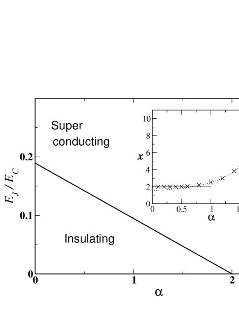
FIG. 1.: The zero-temperature phase diagram in the non-intersecting path approximation. The X’s in the inset show the free energy critical exponent as calculated here. The solid and dotted lines in the inset show the functional form given in Eq. 13.

In this letter we will develop a framework in which these universality classes can be understood in a rigorous, quantitative way. Our formalism, which constitutes an expansion about the insulating state, explicitly preserves the $2\pi$ periodicity of the phase variables, and hence the topological excitations (vortices), which are known to drive the phase transition in the classical limit. We derive a series expansion for the free energy of the associated (2+1)-dimensional statistical mechanics model, which can be approximately summed to all orders. At $T=0$, this is of course just the ground state energy of the quantum system. Strikingly, we find a crossover from universal to non-universal scaling behavior as the coupling strength $\alpha$ to the environment is increased, as shown in the inset of Fig. (1): As long as $\alpha<2/3$, the free energy critical exponent is unchanged from its value for the non-dissipative model, while it varies continuously for $\alpha>2/3$, implying a new universality class. Fig. (2) shows a conjectured renormalization group (RG) flow diagram which we will comment on at the end of the paper.

The model under consideration has been investigated in the past, often by approximations that, in one way or the other, amount to some variant of a self-consistent field approximation, or to linearizing the Josephson coupling term, and hence destroying the $2\pi$ periodicity. However, a recent investigation [7] utilizing a Ginzburg-Landau-Wilson formulation showed results very similar to ours.

A number of mechanisms (see e.g.[7] for references) can give rise to an ungapped electronic density of states, and hence Ohmic damping, in thin-film superconductors. As a scenario that recently gained experimental support[8] we mention the formation of local pools of unpaired electrons due to spatial fluctuations of the order parameter amplitude, caused by impurities. Other possibilities include d-wave high-temperature superconductors with nodal order parameter, coupling to electronic degrees of freedom in the substrate and in the vortex cores, or Andreev scattering. A Josephson array with tunable coupling to the environment in the form of a 2d electron gas has actually been constructed by Clarke et al.[9]

Two-dimensional Josephson junction arrays, as well as superconducting thin films can be modeled as a system of coupled quantum rotors with the Hamiltonian (in the absence of dissipation)

$$H_{XY}=\frac{E_{C}}{2}\sum_{x}n_{x}^{2}+E_{J}\sum_{\left\langle xy\right\rangle}\left[1-\cos(\phi_{x}-\phi_{y})\right],$$ (1)

where the phase $\phi$ of the superconducting order parameter is a compact variable on the interval $[0,2\pi]$, and the Cooper pair number operator $n$ is its canonical conjugate. $E_{C}=(2e)^{2}/C$ and $E_{J}$ are the charging energy and the Josephson coupling energy, respectively. In the above Hamiltonian the ground state is limited to integer filling factors, and more generally we would have to replace $n_{x}^{2}$ by $(n_{x}-\delta)^{2}$, where $\delta$ is some non-integer number. This difference is critical in the non-dissipative model [2], where a non-integer filling factor increases charge fluctuations and hence enhances phase ordering. However, we will see below that this dependence on the filling factor disappears as soon as we include Ohmic dissipation.

FIG. 2.: The conjectured renormalization group flow diagram. The isolated star marks the critical point of the non-dissipative XY transition, the other stars label a critical line. The diamonds mark a line of stable fixpoints at $E_{J}/E_{C}=0$.

In an imaginary time path integral formalism the action for the dissipative system reads

$$S[\phi] = \int_{0}^{\beta}d\tau\left[\frac{1}{2E_{C}}\sum_{x}\dot{\phi}_{x\tau}^{2}-E_{J}\sum_{\left<xy\right>}\cos(\phi_{x\tau}-\phi_{y\tau})\right]$$ (2)

$$+ \frac{1}{2}\sum_{x}\int_{0}^{\beta}d\tau\int_{0}^{\beta}d{\tau^{\prime}}\phi_{x\tau}D(\tau-\tau^{\prime})\phi_{x\tau^{\prime}},$$ (3)

where the last term arises from an integration over the dissipative degrees of freedom [6, 10] and represents Cooper pair breaking processes due to the interaction with the environment. An alternative model would couple the dissipative degrees of freedom to the phase difference across the junction, reflecting the existence of a normal conducting channel between the islands, but will not be considered here. For Ohmic damping the kernel $D(\tau)$ is given by its Fourier transform

$$D(\omega)=\frac{\alpha}{2\pi}|\omega|$$ (4)

for $|\omega|$ less than a high-energy cutoff $\omega_{c}$, which can be approximately set equal to some physical cutoff, such as the bandwidth of localized electron pools. The dimensionless parameter $\alpha$ controls the strength of the dissipative coupling.

In general the compactness of the angular variables causes $\phi$ and $\phi+2\pi$ to be identified, so that $\phi_{\tau}$ is periodic only up to an integer multiple of $2\pi$. We therefore define $\tilde{\phi}_{x\tau}=\phi_{x\tau}-2\pi\beta^{-1}m_{x}\tau_{,}$ where $\tilde{\phi}_{x\tau}$ satisfy periodic boundary conditions and the $m_{x}$ are winding numbers. An infrared divergence in the dissipative term of (3), however, effectively suppresses all nonzero values of $m_{x}$. This leads to another simplification as well: The non-integer filling factors mentioned above give rise to a term $i\delta\int_{0}^{\beta}d\tau\dot{\phi}_{x\tau}=2\pi i\delta m_{x}$ in the action. Hence, as long as winding numbers are suppressed, non-integer filling factors are of no consequence. Intuitively speaking, since in our model the number of Cooper pairs is not conserved, any dependence on the filling factor is washed out.

We now express the partition function as a power series in $E_{J}$:

$$Z = \sum_{n=0}^{\infty}\frac{1}{n!}\prod^{n}_{i=1}\left[\frac{E_{J}}{2}\int_{0}^{\beta}d\tau_{i}\sum_{[x_{i}y_{i}]}\right]\>\int_{0}^{2\pi}D\phi_{x\tau}e^{-S},$$ (5)

$$S = \exp\left\{-S_{0}+i\sum_{x\tau}\int d\tau\eta_{x\tau}\phi_{x\tau}\right\}.$$ (7)

Here $[x_{i}y_{i}]$ indicates a directed bond between two neighboring lattice sites, and the sum runs over all such directed bonds. $\eta_{x\tau}=\sum_{i=1}^{n}\delta(\tau-\tau_{i})(\delta_{x,x_{i}}-\delta_{x,y_{i}})$ can be interpreted as a “charge density,” with $x_{i}$ and $y_{i}$ indicating the position of positive and negative charges, respectively. Each directed pair $[x_{i}y_{i}]$ then constitutes a “dipole.” $E_{J}/2$ plays the role of a fugacity, and $S_{0}$ is the action (3) with $E_{J}=0$. We may call the resulting model the Coulomb dipole model, in analogy to the Coulomb gas model for the resistively shunted Josephson junction[5]. After integrating out the phase variables the action reads

$$S=\frac{1}{2}\sum_{x}\int_{0}^{\beta}d\tau\int_{0}^{\beta}d\tau^{\prime}\eta_{x\tau}v(\tau-\tau^{\prime})\eta_{x\tau^{\prime}},$$ (8)

with

$\displaystyle v(\tau)=\frac{1}{\beta}\sum_{\omega}\frac{e^{i\omega\tau}-1}{E_{C}^{-1}\omega^{2}+D(\omega)},$

where we have subtracted out an infinite constant that enforces “charge neutrality” for each lattice site. For the rest of the paper we will assume $E_{C}\ll\omega_{c}$. Then the interaction potential is well approximated by

$$v(\tau)\simeq-\gamma\ln\left(\frac{\beta\omega^{*}}{\pi}\sin\frac{\pi|\tau|}{\beta}+1\right),$$ (9)

where $\gamma=2/\alpha$. This amounts to replacing the kinetic energy term $E_{C}^{-1}\omega^{2}$ by an effective cutoff $\omega^{*}=E_{C}/2\gamma$. Each term in (7) can be represented by diagrams such as those in Eq. (10). Here each arrow corresponds to a “dipole” as defined above, or in physical terms to a Cooper pair transfer event. Double arrows, such as those in $D_{2}$, indicate two dipoles of opposite orientation occupying the same bond. Similarly, the first diagram in $D_{4c}$ has four dipoles occupying the same bond. As in standard diagrammatic perturbation theory we can use the linked cluster theorem to write the perturbation series for the free energy as a sum over connected diagrams. The diagrams for the first few terms in the expansion

$$f=F/N = f_{0}-2\left(\frac{E_{J}}{2}\right)^{2}D_{2}$$

$$- \left(\frac{E_{J}}{2}\right)^{4}\left\{2D_{4a}+6D_{4b}+\frac{1}{2}D_{4c}\right\}-\cdots$$

follow directly from Eqs. (7) to (9):

\begin{picture}(7.0,1.5)\par\put(0.0,0.6){ \parbox{28.45274pt}{ \par\vskip 0.0pt\vskip 12.0pt plus 3.0pt minus 9.0pt\hbox to469.75499pt{\hskip 0.0pt\hskip 0.0pt plus 1000.0pt$\displaystyle D_{2}=$\hskip 0.0pt plus 1000.0pt}\vskip 12.0pt plus 3.0pt minus 9.0pt\noindent\ignorespaces} } \put(1.5,0.7){\circle*{0.2}} \put(1.9,0.7){\vector(1,0){0.3}} \put(1.9,0.7){\vector(-1,0){0.3}} \put(2.3,0.7){\circle*{0.2}} \put(2.5,0.6){ \parbox{113.81102pt}{ \par\vskip 0.0pt\vskip 12.0pt plus 3.0pt minus 9.0pt\hbox to469.75499pt{\hskip 0.0pt\hskip 0.0pt plus 1000.0pt$\displaystyle=\frac{1}{\beta}\int_{0}^{\beta}d\tau_{1}\int_{0}^{\beta}d\tau_{2}\frac{1}{f^{2}(\tau_{1}-\tau_{2})},$\hskip 0.0pt plus 1000.0pt}\vskip 12.0pt plus 3.0pt minus 9.0pt\noindent\ignorespaces} } \par\end{picture}

\begin{picture}(7.0,1.5)\par\put(0.0,0.8){ \parbox{28.45274pt}{ \par\vskip 0.0pt\vskip 12.0pt plus 3.0pt minus 9.0pt\hbox to469.75499pt{\hskip 0.0pt\hskip 0.0pt plus 1000.0pt$\displaystyle D_{4a}=$\hskip 0.0pt plus 1000.0pt}\vskip 12.0pt plus 3.0pt minus 9.0pt\noindent\ignorespaces} } \put(1.5,1.3){\circle*{0.2}} \put(1.5,0.5){\circle*{0.2}} \put(2.3,1.3){\circle*{0.2}} \put(2.3,0.5){\circle*{0.2}} \put(2.2,1.3){\vector(-1,0){0.4}} \put(1.8,1.3){\line(-1,0){0.2}} \put(1.6,0.5){\vector(1,0){0.4}} \put(2.0,0.5){\line(1,0){0.2}} \put(1.5,1.2){\vector(0,-1){0.4}} \put(1.5,0.8){\line(0,-1){0.2}} \put(2.3,0.6){\vector(0,1){0.4}} \put(2.3,1.0){\line(0,1){0.2}} \put(2.5,0.8){ \parbox{85.35826pt}{ \par\vskip 0.0pt\vskip 12.0pt plus 3.0pt minus 9.0pt\hbox to469.75499pt{\hskip 0.0pt\hskip 0.0pt plus 1000.0pt$\displaystyle=\frac{1}{\beta}\int_{0}^{\beta}\frac{d\tau_{1}\cdots d\tau_{4}}{f_{12}f_{23}f_{34}f_{41}},$\hskip 0.0pt plus 1000.0pt}\vskip 12.0pt plus 3.0pt minus 9.0pt\noindent\ignorespaces} } \par\end{picture}

\begin{picture}(7.0,1.6)\par\put(0.0,1.4){ \parbox{28.45274pt}{ \par\vskip 0.0pt\vskip 12.0pt plus 3.0pt minus 9.0pt\hbox to469.75499pt{\hskip 0.0pt\hskip 0.0pt plus 1000.0pt$\displaystyle D_{4b}=$\hskip 0.0pt plus 1000.0pt}\vskip 12.0pt plus 3.0pt minus 9.0pt\noindent\ignorespaces} } \put(1.5,1.5){\circle*{0.2}} \put(1.9,1.5){\vector(1,0){0.3}} \put(1.9,1.5){\vector(-1,0){0.3}} \put(2.3,1.5){\circle*{0.2}} \put(2.7,1.5){\vector(1,0){0.3}} \put(2.7,1.5){\vector(-1,0){0.3}} \put(3.1,1.5){\circle*{0.2}} \par\put(1.8,1.4){ \parbox{142.26378pt}{ \par\vskip 0.0pt\vskip 12.0pt plus 3.0pt minus 9.0pt\hbox to469.75499pt{\hskip 0.0pt\hskip 0.0pt plus 1000.0pt$\displaystyle-\;(\quad\quad\quad\;)^{2}$\hskip 0.0pt plus 1000.0pt}\vskip 12.0pt plus 3.0pt minus 9.0pt\noindent\ignorespaces} } \par\put(4.1,1.5){\circle*{0.2}} \put(4.5,1.5){\vector(1,0){0.3}} \put(4.5,1.5){\vector(-1,0){0.3}} \put(4.9,1.5){\circle*{0.2}} \par\put(0.0,0.6){ \parbox{227.62204pt}{ \par\vskip 0.0pt\vskip 12.0pt plus 3.0pt minus 9.0pt\hbox to469.75499pt{\hskip 0.0pt\hskip 0.0pt plus 1000.0pt$\displaystyle=\frac{1}{\beta}\int_{0}^{\beta}\frac{d\tau_{1}\cdots d\tau_{4}}{f^{2}_{23}f^{2}_{41}}\left\{\frac{f_{13}f_{24}}{f_{12}f_{34}}-1\right\},$\hskip 0.0pt plus 1000.0pt}\vskip 12.0pt plus 3.0pt minus 9.0pt\noindent\ignorespaces} } \par\end{picture}

\begin{picture}(7.0,1.7)\par\put(0.0,1.4){ \parbox{28.45274pt}{ \par\vskip 0.0pt\vskip 12.0pt plus 3.0pt minus 9.0pt\hbox to469.75499pt{\hskip 0.0pt\hskip 0.0pt plus 1000.0pt$\displaystyle D_{4c}=$\hskip 0.0pt plus 1000.0pt}\vskip 12.0pt plus 3.0pt minus 9.0pt\noindent\ignorespaces} } \par\put(1.5,1.5){\circle*{0.2}} \put(1.9,1.5){\vector(1,0){0.25}} \put(1.9,1.5){\vector(-1,0){0.25}} \put(2.15,1.5){\vector(1,0){0.15}} \put(1.65,1.5){\vector(-1,0){0.15}} \put(2.3,1.5){\circle*{0.2}} \par\put(1.0,1.4){ \parbox{142.26378pt}{ \par\vskip 0.0pt\vskip 12.0pt plus 3.0pt minus 9.0pt\hbox to469.75499pt{\hskip 0.0pt\hskip 0.0pt plus 1000.0pt$\displaystyle-\;2(\quad\quad\quad\;)^{2}$\hskip 0.0pt plus 1000.0pt}\vskip 12.0pt plus 3.0pt minus 9.0pt\noindent\ignorespaces} } \par\put(3.4,1.5){\circle*{0.2}} \put(3.8,1.5){\vector(1,0){0.3}} \put(3.8,1.5){\vector(-1,0){0.3}} \put(4.2,1.5){\circle*{0.2}} \par\put(0.0,0.6){ \parbox{227.62204pt}{ \begin{equation}=\frac{1}{\beta}\int_{0}^{\beta}\frac{d\tau_{1}\cdots d\tau_{4}}{f^{2}_{23}f^{2}_{41}}\left\{\frac{f^{2}_{13}f^{2}_{24}}{f^{2}_{12}f^{2}_{34}}-2\right\}.\end{equation} } } \par\par\end{picture}

Here

$\displaystyle f(\tau)=e^{-v(\tau)}=\left(\frac{\beta\omega^{*}}{\pi}\sin\left|\frac{\pi\tau}{\beta}\right|+1\right)^{\gamma},$

and $f_{ij}$ is a shorthand for $f(\tau_{i}-\tau_{j})$. The subtractions in $D_{4b}$ and $D_{4c}$ are corrections for double counting and are distributed such as to render the diagrams finite in the zero-temperature limit, for $\alpha<2$. Beyond this value each diagram is divergent at $T=0$, reflecting the phase localization transition in a single junction mentioned above.

While for $n\geq 4$ the diagrams are generally very hard to evaluate, there exists a subset which can be computed exactly (within numerical limits) to all orders. The following results are based on this partial summation, and we will comment on the validity of this approximation below. The diagrams we consider are the non-intersecting loops such as $D_{4a}$ in Eq. (10). We then have

$\displaystyle D_{na}=\frac{1}{\beta}\int_{0}^{\beta}\frac{d\tau_{1}\cdots d\tau_{n}}{f_{12}f_{23}\cdots f_{n1}}=\int_{-\infty}^{\infty}\frac{d\omega}{2\pi}\,g^{n}(\omega),$

where (at zero temperature)

$$g(\omega) = \int_{-\infty}^{\infty}d\tau\frac{e^{i\omega\tau}}{\left[|\omega^{*}\tau|+1\right]^{\gamma}}$$

$$= \frac{(\omega^{*})^{-\gamma}}{(i\omega)^{1-\gamma}}\Gamma\left(1-\gamma,i\omega\right)+c.c.$$

The numerical prefactor is equal to the number of translationally distinct self-avoiding polygons of length $n$ on a square lattice, which is known[12] to behave asymptotically as $A_{2n}\sim\mu^{2n}$, with the connective constant $\mu\simeq 2.65$. Hence the free energy is, in this approximation,

$$f=f_{0}-\frac{\omega^{*}}{2\pi}\sum^{\infty}_{n=1}A_{2n}\left(\frac{E_{J}}{2\omega^{*}}\right)^{2n}G_{2n},$$ (11)

where $G_{2n}=(\omega^{*})^{2n-1}\int_{-\infty}^{\infty}d\omega\,g^{2n}(\omega)$ can easily be evaluated numerically. This series constitutes an expansion about a disordered fixpoint of the RG flow diagram. The free energy is singular at the phase transition, and according to the fundamental properties of analytic functions this non-analyticity determines the radius of convergence. We can therefore derive the phase boundary from the asymptotic behavior of the coefficients in (11):

$\displaystyle\left(\frac{E_{J}}{2\omega^{*}}\right)_{c}=\lim_{n\to\infty}\left[\mu^{2n}G_{2n}\right]^{-1/2n}.$

Numerically we find that $G_{n}^{-1/n}\to(\gamma-1)/2$ for large $n$. This relation holds to an accuracy of more than five digits, and is presumably exact. Recalling $\omega^{*}=E_{C}/2\gamma$ and $\gamma=2/\alpha$ we find that the phase boundary is at

$$\left(\frac{E_{J}}{E_{C}}\right)_{c}=\frac{2-\alpha}{4\mu}.$$ (12)

The phase diagram is shown in Fig. (1). In order to assess the quality of the non-intersecting path approximation it is important to realize that we did not omit any terms in the series expansion, but merely replaced the more complicated diagrams with products of simpler ones. For example, the connected piece of diagram $D_{4b}$ is replaced by $(D_{2})^{2}$. To estimate the errors introduced by this approximation we calculated all intersecting diagrams up to sixth order by Monte Carlo integration[11]. We find that in fourth order these corrections change the value of $G_{n}^{1/n}$ by a factor between $1.1$ (for $\alpha\to 0$) and $1.25$ (at $\alpha=2$). For the sixth-order term these factors are $1.12$ ($\alpha\to 0$) and $1.38$ ($\alpha=2$). The second-order term is exact. Because of the relatively small ratios we expect our approximation to overestimate the critical value of $E_{J}/E_{C}$ somewhat, but not to alter the qualitative features of the phase diagram. In particular, it cannot affect the universality classes.

We now turn to the free energy critical exponent. Near the phase transition the singular part of the free energy must be of the form $(1-y)^{x}$, up to logarithmic corrections, where $y=(E_{J}/{E_{J}}_{0})^{2}$ and $x$ is some unknown exponent. Expanding this expression in terms of $y$ we get $f\sim\sum_{n}c_{2n}y^{n}$ with

$\displaystyle c_{2n}=\frac{(-1)^{n}\Gamma(x+1)}{\Gamma(n+1)\Gamma(x-n+1)}.$

The leading asymptotic behavior of the coefficients is given by $\ln c_{2n}\sim-(x+1)\ln n$. The corresponding terms in (11) behave as

$$\ln A_{2n} \sim 2n\ln\mu+(\alpha_{s}-3)\ln n,$$

$$\ln G_{2n} \sim 2n\ln\frac{\gamma-1}{2}-\max\left(\frac{1}{2},\;\frac{1}{\gamma-1}\right)\ln n,$$

where the first relation can be found in the mathematical literature[12] (the exponent $\alpha_{s}$ is conjectured to be $1/2$), and the second relation has been determined numerically. We expect the numerical estimates to be correct at least to three digits precision. Combining these terms we find that the free energy critical exponent is

$$x=\max\left(2,\;\frac{1}{2}+\frac{2}{2-\alpha}\right),$$ (13)

which is shown in the inset of Fig. (1). Due to the high quality of the fits shown we assume that this is an exact result with only minor corrections close to $\alpha=2/3$. The consistency between our results and those of Ref.[7] is emphasized by the scaling relation $z=2x-3$ between $x$ and the dynamical exponent $z$ calculated there. Since all correlation functions and thermodynamic properties of the system, as well as transport properties, can be derived from the free energy, this transition from universal to non-universal scaling behavior should be observable in those quantities as well.

In the language of the renormalization group, the critical point which controls the phase transition of the non-dissipative system has a finite basin of attraction. Since the flow equations are presumably analytic functions of the coupling parameters this implies the existence of an additional critical point on the phase boundary, at $\alpha=2/3$. The continuously varying critical exponent furthermore suggests a line of critical points beyond that value. The first-order RG equations [6] $dE_{J}/dl=(1-2/\alpha)E_{J}$ and $d\alpha/dl=0$ ($l$ is a scale factor for the high-energy cutoff) determine the lower portion of the RG flow diagram, and in particular imply that $E_{J}/E_{C}=0$ constitutes a stable fixed line. Together these arguments lead to the RG flow diagram shown in Fig. (2).

I would like to thank Sudip Chakravarty for enlightening discussions, and Chetan Nayak for useful comments. This work was supported by the grant NSF-DMR-9971138.

REFERENCES

[1] B.G. Orr et al.,
Phys. Rev. Lett. 56, 378 (1986);
H.M. Jaeger et al., Phys. Rev. B 34, 4920 (1986);
D.B. Haviland et al., Phys. Rev. Lett. 62, 2180 (1989).
[2] M.P.A. Fisher et al., Phys. Rev. B 40, 546 (1989).
[3] A. Yazdani and A. Kapitulnik,
Phys. Rev. Lett. 74, 3037 (1995); N. Mason and A. Kapitulnik,
Phys. Rev. Lett. 82, 5341 (1999);
N. Marković et al., Phys. Rev. B 60, 4320 (1999).
[4] L. Geerligs it et al.,
Phys. Rev. Lett. 63, 326 (1989);
H.S.J. van der Zant et al.,
Phys. Rev. Lett. 69, 2971, (1992) and Phys. Rev. B
54, 10081 (1996).
[5] S. Chakravarty, Phys. Rev. Lett. 49,
681 (1982); A. Schmid, Phys. Rev. Lett. 51, 1506
(1983).
[6] S. Chakravarty, G.L. Ingold, S. Kivelson and
A.Luther, Phys. Rev. Lett. 56, 2303 (1986);
S. Chakravarty, G.L. Ingold, S. Kivelson and G. Zimanyi,
Phys. Rev. B 37, 3283 (1988).
[7]
K.H. Wagenblast, A. van Otterlo, G. Schön and G. Zimányi,
Phys. Rev. Lett 78, 1779 (1997).
[8] J.A. Chervenak and J.M. Valles, Phys. Rev. B 59,
11209 (1999); J.M. Valles et al.,
Phys. Rev. Lett. 69, 3567 (1992).
[9] A.J. Rimberg et al.,
Phys. Rev. Lett. 78, 2632 (1997).
[10] A. Caldeira and A. Leggett, Ann. Phys. (N.Y.)
149, 374 (1983); V. Ambegaokar et al.,
Phys. Rev. Lett. 48, 1745 (1982).
[11] K. Völker, unpublished.
[12] “The Self-Avoiding Walk”, N. Madras and G. Slade,
Birkhäuser Boston 1993.