Scaling at the chaos threshold in an interacting quantum dot

Abstract

The chaotic mixing by random two-body interactions of many-electron Fock states in a confined geometry is investigated numerically and compared with analytical predictions. Two distinct regimes are found in the dependence of the inverse participation ratio in Fock space $I$ on the dimensionless conductance of the quantum dot $g$ and the excitation energy $\varepsilon$. In both regimes $I\gg 1$, but only the small-$g$ regime is described by the golden rule. The crossover region is characterized by a maximum in a scaling function that becomes more pronounced with increasing excitation energy. The scaling parameter that governs the transition is $(\varepsilon/g)\ln g$.

PACS numbers: 05.45.+b, 71.10.-w, 73.23.-b

The highly excited atomic nucleus was the first example of a quantum chaotic system, although the interpretation of Wigner’s distribution of level spacings [1] as a signature of quantum chaos came many years later, from the study of electron billiards [2]. While the spectral statistics of the nucleus and the billiard is basically the same, the origin of the chaotic behavior is entirely different [3]: In the billiard chaos appears in the single-particle spectrum as a result of boundary scattering, while in the nucleus chaos appears in the many-particle spectrum as a result of interactions.

The study of the interaction-induced transition to chaos entered condensed matter physics with the realization that a semiconductor quantum dot could be seen as an artificial atom or compound nucleus [4]. A particularly influential paper by Altshuler, Gefen, Kamenev, and Levitov [5] studied the interaction-induced decay of a quasiparticle in a quantum dot and interpreted the broadening of the peaks in the single-particle density of states as a delocalization transition in Fock space. Different scenario’s leading to a smooth rather than an abrupt transition from localized to extended states were considered later [6, 7, 8]. Recent computer simulations [9, 10] also confirm the smooth crossover from localized to delocalized regime for quasiparticle decay.

As emphasized by Altshuler et al. [5], the delocalized regime in the quasiparticle decay problem is not yet chaotic because the states do not extend uniformly over the Fock space. One may study the transition to chaos in the single-particle density of states, but theoretically it is easier to consider instead the mixing by interactions of arbitrary many-particle states. This was the approach taken in Refs. [6, 8, 11, 12, 13, 14], focusing on two quantities: The distribution of the energy level spacings and the inverse participation ratio (IPR) of the wave functions in Fock space. Both quantities can serve as a signature for chaotic behavior, the spacing distribution by comparing with Wigner’s distribution [1] and the IPR by comparing with the golden rule (according to which the IPR is the mean spacing $\delta$ of the many-particle states divided by the mean decay rate $\Gamma$ of a non-interacting many-particle state [12]). Two fundamental questions in these investigations are: 1) What is the scaling parameter that governs the transition to chaos? 2) How sharp is the transition?

In a recent paper [14] one of us presented analytical arguments for a singular threshold governed by the scaling parameter $x=(\varepsilon/g\Delta)\ln g$, where $\Delta$ is the single-particle level spacing, $\varepsilon$ is the excitation energy, and $g$ is the conductance in units of $e^{2}/h$. (Both $\varepsilon/\Delta$ and $g$ are assumed to be $\gg 1$.) In contrast, Georgeot and Shepelyansky [12] argued for a smooth crossover governed by the parameter $y=(\varepsilon/g\Delta)\sqrt{\varepsilon/\Delta}$. (The same scaling parameter was used in Refs. [6, 13].) The parameter $y$ is the ratio of the strength $V\sim\Delta/g$ of the screened Coulomb interaction [5, 15] and the energy spacing $\Delta_{2}\sim(\varepsilon/\Delta)^{-3/2}\Delta$ of states that are directly coupled by the two-body interaction [6]. The parameter $x$ follows if one considers contributions to the IPR that involve the effective interaction of $2,3,4,\ldots$ particles. Subsequent terms in this series are smaller by a factor $(\ln g/g)\Delta_{n}/\Delta_{n+1}$, where $\Delta_{n}\sim(\varepsilon/\Delta)^{-n+1/2}\Delta$ is the spacing of states that are coupled by an effective interaction of $n$ particles [14]. (The large logarithm $\ln g$ appears in the expansion parameter because of the large contribution from intermediate states whose energies are close to the states to be mixed.)

The purpose of this paper is to investigate the interaction-induced transition to chaos by exact diagonalization of a model Hamiltonian. We concentrate on the IPR because for that quantity an analytical prediction exists [14] for the $\varepsilon$ and $g$-dependence. (There is no such prediction for the spacing distribution.) The numerical data is consistent with a chaos threshold at a value of $x$ of order unity.

The model for interacting spinless fermions that we study is the layer model introduced in Ref. [12] and used for the quasiparticle decay problem in Ref. [10]. The Hamiltonian is $H=H_{0}+H_{1}$, with

$$H_{0}=\sum_{j}\varepsilon_{j}c^{\dagger}_{j}c^{\vphantom{\dagger}}_{j},\qquad H_{1}=\sum_{i<j,k<l}V_{ij,kl}c^{\dagger}_{l}c^{\dagger}_{k}c^{\vphantom{\dagger}}_{i}c^{\vphantom{\dagger}}_{j}.$$ (1)

The single-particle levels $\varepsilon_{j}$ are uniformly distributed in the interval $[(j-\frac{1}{2})\Delta,(j+\frac{1}{2})\Delta]$. The interaction matrix elements $V_{ij,kl}$ are zero unless $i,j,k,l$ are four distinct indices with $i+j=k+l$. The (real) non-zero matrix elements have a Gaussian distribution with zero mean and variance $V^{2}=(\Delta/g)^{2}$. The Fock states are eigenstates of $H_{0}$, given by Slater determinants of the occupied levels $k_{1},k_{2},k_{3},\ldots$. The interaction mixes Fock states for which $\sum_{p}k_{p}$ equals a given integer. (Without this restriction the model is the same as the two-body random-interaction model introduced in nuclear physics [16, 17].) The excitation energies of the states with given $k_{1},k_{2},k_{3},\ldots$ lie in a relatively narrow layer (width of order $j^{1/4}\Delta$) around the mean excitation energy $j\Delta$. The number of states in the $j$-th layer is the number of partitions ${\cal P}(j)$ of $j$. For our largest $j=26$ this number is ${\cal P}(26)=2436$, which is still tractable for an exact diagonalization. Without the decoupling of the entire Fock space into distinct layers, such large excitation energies would not be accessible numerically. The layer approximation becomes more reasonable for larger $g$, because then $V\ll\Delta$ so that states from different layers may be regarded as uncoupled.

The inverse participation ratio $I=\sum_{m}|\langle\alpha|m\rangle|^{4}$ of the eigenstate $|\alpha\rangle$ of $H$ is the inverse of the number of eigenstates $|m\rangle$ of $H_{0}$ that have significant overlap with $|\alpha\rangle$. We calculate $I$ as a function of $g$ for different layers $j$, corresponding to a mean excitation energy $\varepsilon=j\Delta$. The IPR fluctuates strongly from state to state and for different realisations of the random matrix $H$. We calculate the averages $\overline{I}$, $\overline{1/I}$ and $\overline{\ln I}$ where the overline $\overline{\cdots}$ indicates an average both over the ${\cal P}(j)$ states $|\alpha\rangle$ in the $j$-th layer and over some $10^{3}$ realisations of $H$. We first consider the logarithmic average $\overline{\ln I}$, for which the fluctuations are smallest.

In Fig. 1 we have plotted the numerical data for the $g$-dependence of $\overline{\ln I}$, for different values of $\varepsilon/\Delta$. In order to compare with the analytical prediction of Ref. [14], we have rescaled the variables such that Fig. 1 becomes a plot of $-y^{-1}\overline{\ln I}$ versus $x$. The prediction is that, in the thermodynamic limit [18], the scaling function $F(x)=-y^{-1}\overline{\ln I}$ depends only on $x$ for $x\lesssim 1$. This scaling behavior can not be checked directly because finite-size effects introduce an additional $\varepsilon$-dependence into the function $F(x)$. This is why we can not directly test whether $x$ or $y$ is the correct scaling parameter. Fortunately, it is possible to include finite-size effects into the scaling function and test the theory in this way.

Applying the method of Ref. [14] for the calculation of $\overline{\ln I}$ one finds that the function $F(x)$ in the thermodynamic limit has the Taylor series

$$F(x)=-y^{-1}\overline{\ln I}=\sum_{n=0}^{\infty}c_{n}x^{n},$$ (2)

with corrections of order $1/\ln g$. All coefficients $c_{n}$ are positive. The scaling behavior (2) is expected to be universal (valid for any model with random two-body interactions), but the coefficients $c_{n}$ are model specific. The first two coefficients for the layer model are

$$c_{0}=\frac{8(2-\sqrt{2})}{\sqrt{3\pi}}=1.53\ \ ,\ \ c_{1}=\frac{81}{25}\sqrt{\frac{2}{\pi}}\,c_{0}=3.95\ .$$ (3)

Finite-size effects introduce an $\varepsilon$-dependence into the coefficients, through the $\varepsilon$-dependence of $K_{n}\equiv(\Delta/\Delta_{n})(\Delta/\varepsilon)^{n-1/2}$. The series expansion of $F(x)$ in terms of the $K_{n}$’s is

$$F(x)=4(\sqrt{2}-1)\sqrt{\pi}K_{2}+36(2-\sqrt{2})K_{3}x+{\cal O}(x^{2}).$$ (4)

For $\varepsilon/\Delta\rightarrow\infty$ we have $K_{2}\rightarrow(2/\pi)\sqrt{2/3}=0.5198$, $K_{3}\rightarrow 6\sqrt{6}/25\pi=0.1871$ and we recover the thermodynamic limit (2). For the excitation energies $\varepsilon/\Delta=15,20,22,24,26$ of the simulation, one has $K_{2}=0.419,0.436,0.439,0.444,0.447$ and $K_{3}=0.0414,0.0536,0.0577,0.0615,0.0648$. The resulting small-$x$ behavior of the scaling function is plotted in Fig. 1 (solid lines) and agrees quite well with the numerical data.

Analytically, the scaling function $F(x)$ is only known for $x\ll 1$. In the simulation, we observe a maximum of $-y^{-1}\overline{\ln I}$ at $x\simeq 1$. The maximum becomes more pronounced with increasing excitation energy. We argue that it is a signature of the transition to chaos, because beyond the maximum, for $x\gtrsim 1$, the IPR is observed to follow the golden-rule prediction (see discussion below)

$$I_{\rm{golden-rule}}=C[j^{5/4}{\cal P}(j)]^{-1}g^{2}.$$ (5)

This golden-rule prediction is shown dashed in Fig. 1, with the coefficient $C\approx 0.51$ as the single fit parameter. (The smallest $\varepsilon/\Delta=15$ was left out of the fit.) Note that $-y^{-1}\ln I_{\rm{golden-rule}}$ has a maximum for an IPR of order unity, hence in the regime of localized states. In contrast, the maximum in $-y^{-1}\overline{\ln I}$ occurs when the IPR is $\ll 1$, hence in the regime of extended states. We now discuss the small and large-$x$ regimes in some more detail.

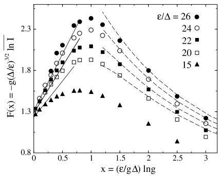
FIG. 1.: Average logarithm of the inverse participation ratio $I$ as a function of the dimensionless conductance $g$, in rescaled variables. The different sets of data points follow from the layer model for different excitation energies $j=\varepsilon/\Delta$. Statistical errors are smaller than the size of the markers. The straight solid lines are the analytical prediction (4) of the scaling theory, without any adjustable parameters. (Only the lines for $\varepsilon/\Delta=15,20$, and $26$ are shown for clarity.) The dashed curves are the golden-rule prediction (5), with a single adjustable parameter (the same for all curves, but the data for $\varepsilon/\Delta=15$ was left out of the fit).

The large-$x$ regime is described by the golden rule $I_{\rm golden-rule}=\delta/\Gamma$, according to which all basis states within the decay width $\Gamma$ of a non-interacting state are equally mixed into the exact eigenstate. This complete mixing amounts to fully developed chaos. For our model the level spacing of the many-particle states in the $j$-th layer is $\delta\sim j^{1/4}\Delta/{\cal P}(j)$ and the Breit-Wigner width is $\Gamma\sim V^{2}/\Delta_{2}\sim j^{3/2}g^{-2}\Delta$, which leads to Eq. (5). One notices in Fig. 1 that for the largest $x$ the data points fall somewhat below the golden-rule prediction. This is due to the finite band width of the layer model. The IPR saturates at $3/{\cal P}(j)$ [9] when the decay width $\Gamma$ becomes comparable to the band width $j^{1/4}\Delta$. The corresponding upper bound on $x$ for the validity of the golden rule is $x\lesssim j^{3/8}\ln g$. The finite band width of the layer model becomes less significant for large $j$, which is why the agreement with the golden rule improves with increasing $j$.

The small-$x$ regime is described by the scaling function $F(x)$. The term of order $x^{n}$ in the Taylor series (2) contains the $n+1$-th order effective interaction $V^{\rm eff}_{n+1}$ between $n+2$ particles and holes. A Fock state in the $j$-th layer contains about $\sqrt{j}$ excited particles and holes [19]. Because this is a large number for $j\gg 1$, the IPR factorizes into a product of independent contributions from $2,3,4,\ldots$ interacting particles,

$$\overline{\ln I}\sim\sum_{n=0}^{\infty}\overline{|V_{n+1}^{\rm eff}|}/\Delta_{n+2}.$$ (6)

A calculation of $\overline{|V_{n+1}^{\rm eff}|}$ leads to Eq. (2). The appearance of the modulus of the matrix element in Eq. (6) is easily understood for the case of only two unperturbed many-particle states interacting via the matrix element $V^{\rm eff}$. The IPR changes by order unity if two Fock states come energetically within a separation $|V^{\rm eff}|$ of each other. The probability of such a near degeneracy is small like $|V^{\rm eff}|/\Delta$. (There is no level repulsion for the many-particle solutions of the non-interacting Hamiltonian.) Because for weak interaction the IPR can change significantly but only with a small probability, the IPR fluctuates strongly. Indeed, in our simulations much larger statistics was necessary in order to reach good accuracy in the small-$x$ regime. (The remaining statistical error in Fig. 1 is smaller than the size of the markers.)

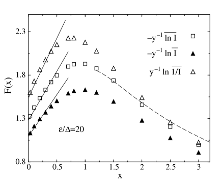
FIG. 2.: Averages $-\overline{\ln I},-\ln\overline{I}$, and $\ln\overline{1/I}$ as a function of $g$, rescaled in the same way as in Fig. 1, for $\varepsilon/\Delta=20$. For small $x$, the three averages follow the scaling theory (7) (solid lines). For large $x$ the averages $-\overline{\ln I}$ and $\ln\overline{1/I}$ follow the golden rule (dashed line).

In Fig. 2 we compare the logarithmic average $\overline{\ln I}$ with the two other averages $\ln\overline{I}$ and $-\ln\overline{1/I}$. Within the small-$x$ regime of validity of Eq. (2) the three averages are related by

$$\overline{\ln I}=2(2-\sqrt{2})\ln\overline{I}=-2(\sqrt{2}-1)\ln\overline{1/I}.$$ (7)

These numerical coefficients do not depend on the number of particles involved in the interaction (cf. the explicit calculation of $\overline{I}$ in Ref. [14]). As one can see in Fig. 2, for $\varepsilon/\Delta=20$, the relation (7) agrees well with the simulation. In the chaotic regime, for large $x$, Eq. (7) is no longer valid. The average $-\ln\overline{1/I}$, which is dominated by the majority of states having a large number of components, is close to $\overline{\ln I}$ at large $x$. The average $\ln\overline{I}$ is dominated by rare states with an anomalously small number of components and falls below the two other averages. This indicates an asymmetric distribution of $\ln I$ in the chaotic regime for the layer model.

So far we have only addressed the question of the scaling variable that governs the transition to chaos. What remains is the question: How sharp is the transition? The singular threshold predicted in Ref. [14] developes only in the thermodynamic limit and would be smoothed by finite-size effects in any simulation. The corresponding non-analyticity of $\overline{\ln I}$ is related to the high-order behavior of the series (2). Since our numerics allows to distinguish only the first two coefficients $c_{0}$ and $c_{1}$, it leaves open the question about the non-analyticity. Still, even if the series (2) would be absolutely convergent, the resulting smooth function of the single variable $x$ could not describe the IPR for large $x$ because it is incompatible with the golden rule $-y^{-1}{\ln I_{\rm golden-rule}}\sim x^{-1}\ln g$. This different scaling behavior for small and large values of $x$ suggests that the peak observed in Fig. 2 would evolve into a singular threshold in the thermodynamic limit. The only way to maintain a smooth crossover would be to introduce a parametrically large interpolating region between the two different scaling regimes. We can not exclude this interpolating region on the basis of the numerical data, however, theoretically [14] there is no indication for such a region.

In summary, by exact diagonalization of a model Hamiltonian we have presented evidence for an interaction-induced transition to chaos in a quantum dot. Upon inclusion of finite-size effects, a good agreement is obtained with the scaling theory of Ref. [14], supporting the assertion that $x=(\varepsilon/g\Delta)\ln g$ is the scaling parameter for the transition. The different behavior of the scaling function for small and large $x$ suggests that the transition would become a singular threshold in the thermodynamic limit.

This work was supported by the Dutch Science Foundation NWO/FOM and by the TMR program of the European Commission. The research of PGS was supported by RFBR, grant 98-02-17905. Discussions with J. Tworzydło are gratefully acknowledged.

REFERENCES

- [1] E. P. Wigner, SIAM Rev. 9, 1 (1967).
- [2] O. Bohigas, M.-J. Giannoni, and C. Schmit, Phys. Rev. Lett. 52, 1 (1984).
- [3] T. Guhr, A. Müller-Groeling, and H. A. Weidenmüller, Phys. Rep. 299, 189 (1998).
- [4] Th. Martin, G. Montambaux, and J. Trân Thanh Vân, editors, Correlated Fermions and Transport in Mesoscopic Systems (Editions Frontières, Gif-sur-Yvette, 1996).
- [5] B. L. Altshuler, Y. Gefen, A. Kamenev, and L. S. Levitov, Phys. Rev. Lett. 78, 2803 (1997).
- [6] P. Jacquod and D. L. Shepelyansky, Phys. Rev. Lett. 79, 1837 (1997).
- [7] A. D. Mirlin and Y. V. Fyodorov, Phys. Rev. B 56, 13393 (1997).
- [8] P. G. Silvestrov, Phys. Rev. Lett. 79, 3994 (1997).
- [9] C. Mejía-Monasterio, J. Richert, T. Rupp, and H. A. Weidenmüller, Phys. Rev. Lett. 81, 5189 (1998).
- [10] X. Leyronas, J. Tworzydło, and C. W. J. Beenakker, Phys. Rev. Lett. 82, 4894 (1999).
- [11] V. V. Flambaum and F. M. Izrailev, Phys. Rev. E 56, 5144 (1997).
- [12] B. Georgeot and D. L. Shepelyansky, Phys. Rev. Lett. 79, 4365 (1998).
- [13] R. Berkovits and Y. Avishai, Phys. Rev. Lett. 80, 568 (1998).
- [14] P. G. Silvestrov, Phys. Rev. E 58, 5629 (1998).
- [15] Ya. M. Blanter, Phys. Rev. B 54, 12807 (1996).
- [16] J. B. French and S. S. M. Wong, Phys. Lett. B 33, 449 (1970); 35, 5 (1971).
- [17] O. Bohigas and J. Flores, Phys. Lett. B 34, 261 (1971); 35, 383 (1971).
- [18] By the thermodynamic limit we mean the limit of high excitation energy and large conductance, namely, at fixed .
- [19] The probability to find the single-particle level (with excitation energy ) occupied in a Fock state is . It has the form of a Fermi-Dirac distribution at an effective temperature . This formula, though formally valid only in the thermodynamic limit , describes well the average occupation number already at the values of our simulations.