Depinning of kinks in a Josephson-junction ratchet array

Abstract

We have measured the depinning of trapped kinks in a ratchet potential using a fabricated circular array of Josephson junctions. Our ratchet system consists of a parallel array of junctions with alternating cell inductances and junctions areas. We have compared this ratchet array with other circular arrays. We find experimentally and numerically that the depinning current depends on the direction of the applied current in our ratchet ring. We also find other properties of the depinning current versus applied field, such as a long period and a lack of reflection symmetry, which we can explain analytically.

]

I Introduction

Disorder and noise are not always undesirable in physical systems. Inhomogeneity has been shown to control certain types of spatiotemporal chaos[1], while noise can lead to an enhancement of the signal-to-noise ratio because of stochastic resonance [2]. Another more recent counterintuitive result is that of transport of a Brownian particle in a ratchet potential [3]. Though initially proposed as a model for molecular motors in biological organisms [4], ratchets can also serve as a model to study dissipative and stochastic processes in nanoscale devices.

A ratchet potential is a periodic potential which lacks reflection symmetry (in 1D $V(x)\neq V(-x)$, see Figure 1). A consequence of this symmetry breaking is the possibility of rectifying non-thermal, or time correlated, fluctuations [5]. This can be understood intuitively. In Fig. 1, it takes a smaller dc driving force to move a particle from a well to the right than to the left. In other words, the spatial symmetry of the dc force is broken. Under an ac drive (so-called “rocking ratchets”) or time-correlated noise, particles show net directional motion in the smallest slope direction. This effect can be used in devices in which selection of particle motion is desired.

Because of this effect, ratchet engines have been proposed as devices for phase separation [6], and very recently as a method of flux cleaning in superconducting thin films [7]. A ratchet mechanism has also been proposed as a method to prevent mound formation in epitaxial film growth [8].

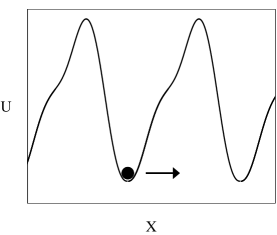
FIG. 1.: Example of a ratchet potential. The particle sitting on the well requires less force to move through the first peak to the right than to move to the left. Therefore, there is a preferred direction of motion.

Josephson junctions are solid state realizations of a simple pendulum. By coupling them, it is possible to make a physical realization of model systems such as the Frenkel-Kontorova model for dislocations [9, 10] or the 2-D X-Y model [11] for phase transitions. In particular, a parallel Josephson array (see Fig. 2) is a discrete version of the sine-Gordon equation and it has been used to experimentally study soliton (usually referred to as kinks, vortices or fluxons) dynamics on a discrete lattice [10].

In parallel arrays, kinks behave as particles in which the idea of Brownian rectification can apply. The applied current is the driving force. If the kink experiences a ratchet potential, then the current needed to move the kink in one direction is different than the current to move it in the opposite direction.

In this paper, we will show that we can design almost any type of 1D pinning potential in a parallel Josephson array by choosing an appropriate combination of junction critical currents and plaquette areas. Indeed, it has been shown [12] that two alternating critical currents and plaquettes areas are enough to provide a ratchet potential for fluxons. As we will show below, this is not the only possible design for a ratchet potential.

With only an ac driving current these arrays show dc voltage steps of stability at multiples of the external ac drive amplitude. This occurs when the equivalent ac driving force becomes commensurate with the period of the ratchet potential. This behavior could open the possibility of using these arrays for a voltage standard device or a microwave detector without a dc bias current. Moreover, the same ideas of flux cleaning underlying reference [7] could be applied to 2D arrays using the designs described here.

The paper is organized into 5 sections. Section II introduces the theoretical framework for the study of an inhomogeneous parallel Josephson arrays. We find that inhomogeneous arrays present a long periodicity with respect to the number of kinks in the array. To test the theory, we have designed four different Josephson junction rings and measured the depinning current of the array versus the applied magnetic field. The experimental results are shown in section III. In section IV we discuss some of the properties of the model and show that they agree well the experimental results. We also show that a combination of three different critical current junctions is sufficient to design a ratchet potential. In section V we present the conclusions of our work and propose a number of new experiments.

II Theoretical framework

A Circuit model

Figure 2 shows the circuit diagram for an array of Josephson junctions. Each junction is marked by an “$\times$” and we will connect $N$ junctions in parallel with short wires as shown. Coupling of the junctions occurs through the geometrical inductances of the cells. We will neglect all mutual inductances and consider only the self-inductance of each cell $L_{j}$. The induced flux in each cell is then $L_{j}$ times the mesh current of the cell which in this simple geometry can be easily seen to equal the current through the top horizontal link $I^{j}_{b}$. We will use $I_{ext}$ for the uniformly applied external bias current per junction as shown in Fig. 2. We then define the mesh current as the current passing through this top horizontal wire. With this definition we can place the loop self-inductance $L_{j}$ on the top horizontal link. We emphasize that this inductance is not the wire inductance, but the self-inductance of the cell so that only one such element is needed per cell.

$.\hskip 4.33601pt.\hskip 4.33601pt.$$.\hskip 4.33601pt.\hskip 4.33601pt.$$I_{ext}$ $I_{c}^{j-1}$  ${L_{j-1}}$  $I_{c}^{j}$  ${L_{j}}$  $I_{c}^{j+1}$  ${L_{j+1}}$  $I_{c}^{j+2}$ $.\hskip 4.33601pt.\hskip 4.33601pt.$$.\hskip 4.33601pt.\hskip 4.33601pt.$

FIG. 2.: Circuit diagram for an inhomogeneous parallel Josephson array. Each junction has a critical current $I_{c}^{j}$ and each cell has an inductance of $L_{j}$.

The junctions will be modeled by the parallel combination of an ideal Josephson junction with a critical current of $I_{c}^{j}$, a capacitor $C_{j}$, and a resistance $R_{j}$. The ideal Josephson junction has a constitutive relation of $I_{j}=I_{c}^{j}\sin\varphi_{j}$ where $\varphi_{j}$ is the gauge-invariant phase difference of the junction. When there is a voltage across the junction, $v_{j}$, then $v_{j}=(\Phi_{0}/2\pi)d\varphi_{j}/dt$. Since we will have $N$ parallel junctions, in our array $j=1$ to $N$.

The circuit equations result from applying current conservation and flux quantization[13]. Current conservation at the top node of junction $j$ yields

$$C_{j}\dot{v}_{j}+{v_{j}\over R_{j}}+I_{c}^{j}\sin\varphi_{j}=I_{ext}+I_{b}^{j}-I_{b}^{j-1}$$ (1)

Flux quantization of cell $j$ yields

$${\Phi_{0}\over 2\pi}(\varphi_{j+1}-\varphi_{j})=\Phi_{j},$$ (2)

where $\Phi_{j}$ is the total flux in cell $j$.

Due to the linearity of Maxwell’s equations, $\Phi_{j}$ can be decomposed into two parts: the induced flux $\Phi_{ind}^{j}$, and the external flux $\Phi_{ext}^{j}$ which is the applied field $B_{ext}$ times the cell area $A_{j}$. The induced flux is simply $L_{j}$ times the mesh current of the cell, which has been defined to equal $I_{b}^{j}$. Then,

$$C_{j}\dot{v}_{j} + {v_{j}\over R_{j}}+I_{c}^{j}\sin\varphi_{j}=I_{ext}+F_{j}$$ (4)

$$+{\Phi_{0}\over 2\pi}\left[{1\over L_{j}}(\varphi_{j+1}-\varphi_{j})+{1\over L_{j-1}}(\varphi_{j-1}-\varphi_{j})\right]$$

with $F_{j}=(\Phi_{ext}^{j-1}/L_{j-1}-\Phi_{ext}^{j}/L_{j})$.

This circuit is realizable by varying cell and junction areas. The cell area $A_{j}$ will determine the self-inductance. If $W$ is the width of the cell and $\Delta x_{j}$ is its length then $L_{j}\approx\mu_{0}\Delta x_{j}$ as long as $W\sim\Delta x_{j}$. Since $\Phi_{ext}^{j}=W\Delta x_{j}B_{ext}$, we see that $\Phi_{ext}^{j}/L_{j}\approx WB_{ext}/\mu_{0}$ and is approximately constant for all $j$. The junction area determines $I_{c}^{j},C_{j}$, and $R_{j}$ but they are not independent since the capacitance and critical current are linearly proportional to the junction area and the resistance is inversely proportional to the junction area. The $I_{c}^{j}R_{j}$ product and the $I_{c}^{j}/C_{j}$ ratio of each junction are constant for every junction.

We will normalize all the currents by $I_{c}^{\star}=\max(I_{c}^{j})$ and time by $\tau=\sqrt{\Phi_{0}C_{\star}/2\pi I_{c}^{\star}}$ where $C_{\star}=\max(C_{j})$. Then,

$$h_{j}{\cal N}(\varphi_{j})= i_{ext}+f_{j}$$ (6)

$$+\lambda_{j}(\varphi_{j+1}-\varphi_{j})+\lambda_{j-1}(\varphi_{j-1}-\varphi_{j})$$

where ${\cal N}(\varphi_{j})=\ddot{\varphi}_{j}+\Gamma\dot{\varphi}_{j}+\sin\varphi_{j}$ [14]. The ratio of critical currents is $h_{j}=I_{c}^{j}/I_{c}^{\star}$ and the inductances are normalized as $\lambda_{j}=\Phi_{0}/2\pi I_{c}^{\star}L_{j}$. Finally, $f_{j}=2\pi f(\lambda_{j-1}A_{j-1}/A_{\star}-\lambda_{j}A_{j}/A_{\star})$, where $f$ is the frustration $B_{ext}A_{\star}/\Phi_{0}$. We have used $A_{\star}=\max(A_{j})$.

To complete the system we need to specify the boundary conditions. There are two types: open, if the junctions form a linear row; and periodic, if the junctions form a closed ring.

For the open boundary condition we set $\lambda_{0}=A_{0}=0$ in Eq. 6 for junction $j=1$. At the other end of the array, $j=N$, we set $\lambda_{N}=A_{N}=0$.

For the periodic boundary conditions we let $\lambda_{0}=\lambda_{N}$ and $A_{0}=A_{N}$. Furthermore, a circular system poses a topological constraint on $\varphi_{j}$ since they are angular variables and have $2\pi$ periodicity: $\varphi_{j+N}=\varphi_{j}+2\pi M$. In particular $\varphi_{0}=\varphi_{N}-2\pi M$ and $\varphi_{N+1}=\varphi_{1}+2\pi M$. Here $M$ is referred to as the winding number and represents the number of kinks in the system.

In this paper we will discuss systems with periodic boundary conditions. Since the product $\lambda_{j}A_{j}$ is roughly constant throughout the array we consider $f_{j}=0$ in the simulations of the rings we present [15]. We have checked numerically that for the experiments reported here, these terms do not significantly alter our results.

B Symmetries

The system of equations (6) presents an odd inversion symmetry under the change $M\to-M$, $\varphi_{i}\to-\varphi_{i},$ and $i_{ext}\to-i_{ext}$ as is expected from Maxwell’s equations. The response of the array to an external current will reflect this symmetry. In particular, $I_{dep}(-M)=-I_{dep}(M)$. Here, $I_{dep}$ is the maximum value of the applied current for which a solution $\dot{\varphi_{j}}=0$ can not be sustained in the presence of a positive or negative external current. To refer to this odd inversion symmetry we will use the notation $I_{dep-}(-M)=I_{dep+}(M)$ where $I_{dep\pm}$ refers to the absolute value of the depinning current as the external current is increased or decreased from zero.

Another symmetry of the equations refers to the periodicity of the system when varying the number of kinks in the array. In the case of a regular ring (all the cells and junctions are equal) this period $T$ is equal to the number of junctions, $N$ [16].

A method of calculating the periodicity in $M$ for the general case studied here is to use the simple transformation

$$\psi_{j}=\varphi_{j}+2\pi m_{j}$$ (7)

where $m_{j}$ are integers. The equations of motion in the new variables are the following

$$h_{j}{\cal N}(\psi_{j}-2\pi m_{j})=\lambda_{j}(\psi_{j+1}-\psi_{j})+\lambda_{j-1}(\psi_{j-1}-\psi_{j})$$ (8)

$$-2\pi\lambda_{j}(m_{j+1}-m_{j})-2\pi\lambda_{j-1}(m_{j-1}-m_{j})+i_{ext}+f_{j}$$ (9)

where ${\cal N}(\psi_{j}-2\pi m_{j})={\cal N}(\psi_{j})$. The new boundary conditions are

$$\psi_{j+N}=\psi_{j}+2\pi(M+T)$$ (10)

where $T=m_{j+N}-m_{j}$. Thus after the transformation (7) we recover the same equations as (6) but with the number of kinks equal to $M+T$ so that the equations are periodic in the number of kinks in the array with a period $T$.

To calculate $T$ we take out the $m_{j}$ dependence on the right hand side of Eq. 9 by choosing $m_{j}$ such that $\lambda_{j}(m_{j+1}-m_{j})+\lambda_{j-1}(m_{j-1}-m_{j})=0$. Remarkably, the resulting period is independent of $h_{j}$ and only depends on the ratio between the consecutive $\lambda^{\prime}s$. In the appendix we find a formula for the periodicity in the number of kinks for the general system.

Here we are going to develop the case of a ring that was measured: a ring with an even number of junctions and with alternating cell areas. In this case there are only two $\lambda^{\prime}s$ involved. Let $\lambda_{j}=\lambda_{1}(\lambda_{2})$ for $j$ odd(even) and $\lambda_{1}/\lambda_{2}=p/q$. If we let $(m_{j-1}-m_{j})=-q$ and $(m_{j+1}-m_{j})=p$ (for even $j$ for instance), we satisfy the above condition.

The period is calculated from the new boundary conditions:

$$T=m_{N+1}-m_{1}=(p+q)N/2.$$ (11)

For the regular array $p=q=1$ and we recover the expected result of $T=N$. Also, we note that in order to have a finite period we need the ratios between $\lambda^{\prime}s$ to be rational numbers. This condition will almost never be satisfied in a real experiment. Thus we see that a simple design of alternating cell areas can result in an arbitrarily long period (that could be equal to $\infty$) when varying the number of kinks in the array.

A similar calculation can be made for the case of an open array. As no topological constraint for the phases can be imposed, the number of kinks in the array does not appear in our equations. We consider instead the periodicity of the system with the external field. In this case, the periodicity depends on the ratio between the cell areas instead of the ratio between the inductances. It can be shown that the period in $f=B_{ext}A_{\star}/\Phi_{0}$ is equal to $q$, where $A_{2}/A_{1}=p/q$ and $A_{1}=A_{\star}$.

III Experimental results

We have designed and fabricated the four different rings (a), (b), (c) and (d) schematically shown in Fig. 3. The rings are fabricated with a Nb-Al₂O_x-Nb tri-layer technology with a junction critical current density of $1\,{\rm kA/cm^{2}}$. The current is injected through bias resistors in order to be distributed as uniformly as possible. We measure the dc voltage across a single junction [17] and each ring consists of $N=8$ junctions.

FIG. 3.: The four different measured arrays: (a) regular ring, $h_{j}=1$ and $\lambda_{j}=0.11$ (b) ring with alternating critical currents, $h_{j}=1$ and $h_{j+1}=0.43$, $\lambda_{j}=0.043$, (c) ring with with alternating cell area, $h_{j}=1$, $\lambda_{j}=0.08$ and $\lambda_{j+1}=0.15$ (d) ratchet ring with alternating critical currents and cell areas, $h_{j}=1$, $h_{j+1}=0.43$, $\lambda_{j}=0.035$, and $\lambda_{j+1}=0.06$. These parameters are calculated at $T=0\,K$.

Fig. 3(a) is a regular ring with equal critical currents and plaquette areas. Fig. 3(b) has alternating critical currents with a ratio of 0.43. Fig. 3(c) has alternating plaquette areas with a ratio of $\lambda^{\prime}s$ of 1.8. Finally, Fig. 3(d) has both alternating critical currents and alternating plaquette areas. It will be shown experimentally that only (d) has a ratchet pinning potential.

The outer diameter of each ring is $36\,{\rm\mu m}$ with an area $\sim 4070\,{\rm\mu m}^{2}$. The inner diameter is $18\,{\rm\mu m}$ and it consists of an island of niobium that is used to extract the applied current. The rings also have either small junctions ($3\times 3\,{\rm\mu m^{2}}$) or alternating small and large junctions ($4.25\times 4.25\,{\rm\mu m^{2}}$). The designed $I_{c}$ ratio is 0.5, but in practice the junction areas have rounded corners and experimentally we find the $I_{c}$ ratio to be 0.43. We vary the cell inductance by alternating the cell area. In this case, the angles of the cells are $60^{\circ}$ and $30^{\circ}$.

Both $\Gamma$ and $\lambda$ are mostly determined from material properties of the samples and the junction $I_{c}$. Since $I_{c}$ varies with temperature, both parameters can be experimentally controlled to some extent. In general $\Gamma$ and $\lambda$ can be made larger by up to a factor of 10 by raising the sample temperature. As the temperature reaches $T_{c}$, however, most of the measured features become too smeared to be distinguished.

The temperature dependence of $I_{c}$ is modeled well by the standard Ambegaokar-Baratoff relation with $I_{c}(0)R_{n}=1.9\,{\rm mV}$ [18]. We find that $I_{c}(0)=95\,{\rm\mu A}$ for the small junctions and $I_{c}(0)=224\,{\rm\mu A}$ for the larger junctions. We will normalize all our parameters with the largest $I_{c}$ of a given ring. From the above values, we can estimate $\rm\Gamma(0)=0.17$ which, due to the constant $I_{c}R_{n}$ product, is independent of junction area. The inductances are estimated from a numerical package that extracts inductances from complex 3-D geometries of conductors [19]. In this sample the loop inductance is ${L}=23.5\,{\rm pH}$ for the small cells and ${L}=42.6\,{\rm pH}$ for the large ones [arrays (c) and (d)]. For the cells in rings (a) and (b) ${L}=33.5\,{\rm pH}$. To calculate dimensionless penetration depth $\lambda(0)=\Phi_{0}/2\pi LI_{c}(0)$ we use $I_{c}=95\,{\rm\mu A}$ if the ring only has small junctions [(a) and (c)] and for those rings that also have large junction [(b) and (d)] we use $224\,{\rm\mu A}$.

The current-voltage, IV, curves are measured by applying a perpendicular magnetic field of 0 to 300 mG through a magnetic coil that is mounted on the radiation shield of our probe. We heat the sample above $T_{c}=9.2\,{\rm K}$ and cool down to a temperature $T<T_{c}$. We cool our ring in the presence of a flux that corresponds to approximately $M$ flux quanta. Flux quantization will cause the expulsion of extra flux so that the ring contains exactly $M$ flux quanta after undergoing a superconducting transition.

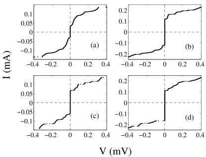
FIG. 4.: Sample IV curves for the four rings considered in Fig. 3 ((a) corresponds to Fig. 3(a) and so on). Rings (a), (b), and (c) have symmetric IV’s as the current is swept in the positive and negative direction. The measurements correspond to $M=1$. Ring (d) is the ratchet ring as can be seen from the difference in the depinning current in the positive and negative direction.

Figure 4 shows typical IV’s for the different rings shown in Fig. 3. Fig. (a) is for a regular ring when $M=1$. The IV is symmetric with respect to applied current direction. As the current is increased from the superconducting state the voltage remains at zero. We define the depinning current when the array has a voltage greater than a threshold of $1.5\,\mu{\rm V}$. Our computer controlled equipment also corrects for any voltage drift of our amplifiers. As the current increases beyond the depinning value, there is a sequence of voltage steps where as the current increases the voltage remains relatively constant. There are at least two mechanisms that can cause these steps: resonances between the circulating kink and radiated linear waves, and instabilities of the whirling branch[10]. We have verified that the voltage positions correspond to these two mechanisms.

Figure 4(b) is a ring with alternating critical currents when $M=1$. We again see that the IV is symmetric with respect to current direction and that there are voltage steps. These steps are of the same origin as in the regular ring. However, in this ring the linear dispersion relation that determines the resonance condition is split into two branches. This splitting is analogous to the optical and acoustic branches of a crystal with a two atom basis. Fig. (c) is a ring with alternating areas. The characteristics are similar to that of ring (b) including a splitting of the linear dispersion relation. Since for these three rings $I_{dep+}=I_{dep-}$, we can infer that the kink is traveling in a symmetric pinning potential as theoretically expected.

Figure 4(d) shows an IV for the ring with both alternating critical currents and areas. The IV of this ring is qualitatively different from the other rings due to the ratchet nature of the pinning potential. We see that $I_{dep}$ in the positive direction is $\sim 65\%$ of the depinning current in the negative direction. We also note that there are different voltage steps excited in the up and down direction. The steps are of the same nature as the explained resonances above and there is also a splitting of the dispersion relation. In the rest of the article we will focus on $I_{dep}$ measurements as a signature for ratchet behavior in our arrays.

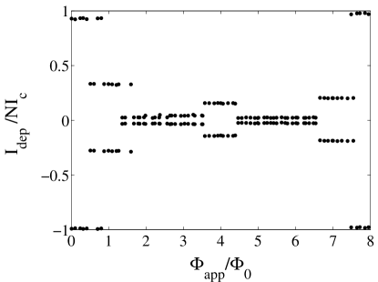
FIG. 5.: Measured critical currents vs. applied flux for a regular ring. To calculate applied flux, we multiply the applied field by the ring area. A constant offset has also been subtracted to account for the ambient magnetic field. The measurement was done at $T=8.8\,{\rm K}$ with $\Gamma\approx 0.5$ and $\lambda\approx 0.9$.

Figure 5 shows a measurement of the depinning current vs. applied flux for the regular ring shown in Fig. 3(a). The temperature is $8.8\,{\rm K}$, $\Gamma=0.5$ while $\lambda=0.9$. Each plateau represents a different number of kinks trapped in the ring. This is a direct result of flux quantization: The ring only allows integer number of flux quanta even if we have applied slightly more or less flux. Since $N=8$ and this ring has a symmetric pinning potential, we expect $I_{dep+}=I_{dep-}$ (no ratchet effect), and a period of 8 as can be seen in the measurements. We also see that $I_{dep}$ has a reflection symmetry about $M=T/2$.

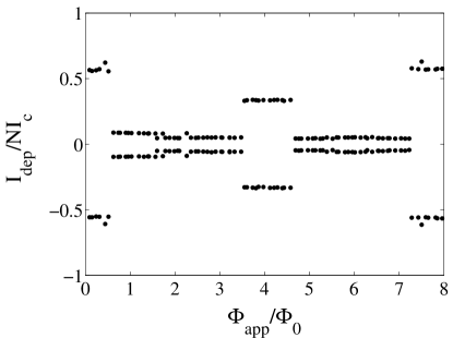
FIG. 6.: Measured critical currents vs. applied flux for a ring with alternating critical currents. The applied flux was calculated as described in Fig. 5. The measurement was done at $T=9\,{\rm K}$ with $\Gamma\approx 0.7$ and $\lambda\approx 0.9$.

When we alternate the critical currents in our ring we expect the same qualitative features of $I_{dep}$ as in the regular ring. Figure 6 shows a measurement of the depinning current vs. applied flux for the ring shown in Fig. 3(b) which has alternating critical currents. There are plateaus corresponding to different values of $M$ just as in the regular ring and there is up-down symmetry and periodicity with $M=8$ as expected, and a reflection symmetry about $M=4$.

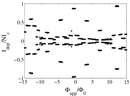
FIG. 7.: Measured critical currents vs. applied flux for a ring with alternating cell areas. The applied flux was calculated as described in Fig. 5. The measurement was done at $T=9\,{\rm K}$ with $\Gamma\approx 0.7$ and $\lambda_{l}\approx 0.7$ and $\lambda_{s}\approx 1.3$.

If we make all the critical currents constant and vary only the cell area as in Fig. 3(c), then we alternate the values of $\lambda$ but the pinning potential remains symmetric. At $T=9\,{\rm K}$, $\lambda_{l}$ for the large cell is $\approx 0.7$ and $\lambda_{s}$ for the small cell is $\approx 1.3$. The result of measuring $I_{dep}$ is shown in Fig. 7. As expected the data is symmetric with respect to current direction so kinks are not traveling in a ratchet pinning potential. However, unlike in the previous rings, $I_{dep}$ is no longer periodic with $M=8$. As shown in section II B, the period will depend on the ratio of the inductances. For our geometry $L_{1}/L_{2}\approx 1.8$ or $9/5$ which implies a period of 56. However, in any physical array the inductance ratio is rarely going to be exactly a ratio of small numbers. Just on physical grounds we expect a very large period, if any, in the experiments. In Fig. 7 we have measured the depinning current from $M=-15$ to $M=15$ and though there is some apparent self-similarity in the data, it is not periodic. Though there is no period, we can still prepare our ring systematically with $M=1$, 2, 3, etc. by counting the plateaus. But instead of $M=1$ and $M=1+N$ yielding the same dynamical system as in the regular ring, they are now distinguishable.

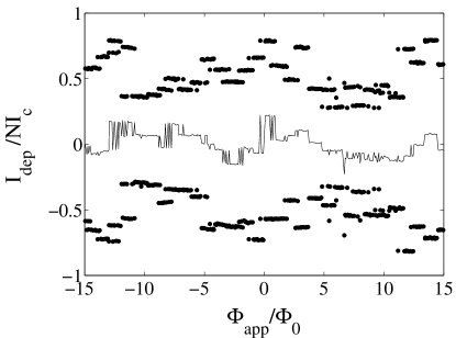
FIG. 8.: Measured critical currents vs. applied flux for a ratchet ring. The applied flux was calculated as described in Fig. 5. The measurement was done at $T=8.8\,{\rm K}$ with $\Gamma\approx 0.5$ and $\lambda_{l}\approx 0.3$ and $\lambda_{s}\approx 0.6$. The line varying about $I_{dep}=0$ is the difference between $I_{dep+}$ and $I_{dep-}$.

When we alternate both the critical current and the cell inductances as in Fig. 3(d), it is possible to form a ratchet pinning potential (see Figure 1). Fig. 8 shows an experiment on such a ring. Since the period depends on the inductance ratio, we experimentally expect a very long period. This is borne out by the data as there is no sign of a period in the range from $M=-15$ to 15. We also expect that $I_{dep+}\neq I_{dep-}$ since the kink is traveling in a ratchet pinning potential. The line shown in the center of the figure varying about $I_{dep}=0$ is the difference between the $I_{dep+}$ and $I_{dep-}$. Clearly, the force to move kinks in one direction is different than the force to move it in the opposite direction. The magnitude and direction of this ratchet effect depends on the number of kinks in the system.

As a further test of the symmetries and periods of the experiments, we have numerically integrated Eq. 6 using a variable step size explicit 4th order Runge-Kutta method. The kink number $M$ is set in the boundary junctions. The initial conditions are $\varphi_{j}=2\pi Mj/N$. That is, we stretch the kinks across the full array at the start of the simulation. We then sweep the applied current in the positive direction until a voltage develops in the array and calculate $I_{dep+}$. We repeat the procedure while sweeping the current in the negative direction to calculate $I_{dep-}$.

Figure 9 shows the simulations with parameters similar to those of the experiments. Both Fig. 9(a) and Fig. 9(b) have alternating $\lambda^{\prime}s$ with $\lambda_{j}=0.3$ and $\lambda_{j+1}=0.54$ for $j$ odd. The inductance ratio is $0.54/0.3=9/5$ so using Eq. 11 the expected period is $T=56$. We find this period in the simulations. Fig. 9(a) has $h_{j}=1$ so we expect the depinning current to be up-down symmetric, i.e. no ratchet effect, as can be seen in the data. Since we always have an odd inversion symmetry [$I_{dep+}(M)=I_{dep-}(-M)=I_{dep-}(T-M)$], $I_{dep}$ is symmetric about $M=56/2=28$. This reflection symmetry of $I_{dep}$ about $T/2$ is generic for any array that is not ratchet since it is a direct consequence of the up-down symmetry of the currents. We also find this symmetry in the experiments of non-ratchet arrays.

Fig. 9(b) has junctions with two alternating critical currents ($h_{j}=1$ and $h_{j+1}=0.43$ for $j$ odd) as well as two alternating $\lambda$’s ($\lambda_{j}=0.3$ and $\lambda_{j+1}=0.54$ for $j$ odd). We now expect the kinks to travel in a ratchet pinning potential so that $I_{dep+}$ does not equal $I_{dep-}$, though $I_{dep}$ still has an odd inversion symmetry. Just as in the experiments we see that the effect of the ratchet, and rectification direction, depends on the number of kinks. Also, $I_{dep}$ does not have the expected reflection symmetry about $T/2$. In summary, the simulations show the same features as the experiments and also agree quantitatively with our predictions.

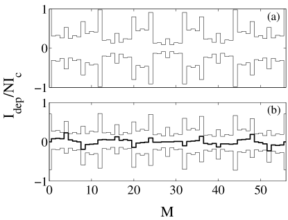
FIG. 9.: (a) Simulation for $N=8$ ring with only alternating $\lambda$’s of $\lambda_{l}=0.3$ and $\lambda_{s}=0.54$, and $h_{j}=1$. (b) Simulation for $N=8$ ratchet ring with both alternating $\lambda$’s of $\lambda_{j}=0.3$ and $\lambda_{j+1}=0.54$ and critical currents of $h_{j}=1$ and $h_{j+1}=0.43$. Line shown about $I_{dep}=0$ is the difference between $I_{dep+}$ and $I_{dep-}$.

IV Discussion

The equations developed in section II describe kink propagation through a discrete inhomogeneous medium. In this section we will try to get a better understanding of the system by briefly analyzing the continuous limit of our discrete equations. We will then go back to our discrete equations and approximate the pinning potential for a single kink. With the analysis, it will become apparent how it is possible to construct many types of pinning potentials, including ratchet ones, in the inhomogeneous array.

To derive the continuous limit of the equations, let $2{\bar{\lambda}}_{j}=\lambda_{j}+\lambda_{j-1}$ and $\delta\lambda_{j}=\lambda_{j}-\lambda_{j-1}$. Substituting in Eq. 6, we get

$$h_{j}{\cal N}(\varphi_{j})={\bar{\lambda}}_{j}\partial_{xx}\varphi_{j}+\delta\lambda_{j}\partial_{x}\varphi_{j}+f_{j}+i_{ext}$$ (12)

where $\partial_{xx}\varphi_{j}=\varphi_{j+1}-2\varphi_{j}+\varphi_{j-1}$ represents a discrete Laplacian while $\partial_{x}\varphi_{j}=(\varphi_{j+1}-\varphi_{j-1})/2$ is just the center difference of the first order derivative. To arrive at a continuous limit we expand our variables as Taylor series in $\Delta x_{j}$. The cell area is $W\Delta x_{j}$ while the cell inductance $L_{j}=G\Delta x_{j}$ as $\Delta x_{j}\to 0$ where $G$ is a geometric constant. Therefore $f_{j}=0$ as $\Delta x_{j}\to 0$ and the discrete operators are replaced by their continuous derivatives

$$h(x){\cal N}(\varphi) = \lambda(x)\partial_{xx}\varphi+\partial_{x}\lambda(x)\partial_{x}\varphi+i_{ext}$$ (13)

$$= {\partial_{x}}\left(\lambda(x){\partial_{x}}\varphi\right)+i_{ext}$$ (14)

If $\lambda$ and $h$ are constant then we have the usual sine-Gordon equation. In this case the equations have a reflection symmetry and it is not possible to have a ratchet pinning potential. If $\lambda$ is dependent on position, the spatial coupling is analogous to inhomogeneous diffusion, anisotropic heat conduction, or waves traveling in an anisotropic medium. We also note that $f_{j}$ in the discrete equations is essentially a perturbation to the continuous model that is dependent on the exact discretization employed and is usually small. Thus, in order to get a ratchet pinning potential, there are three ways to break the reflection symmetry of the equations: with an appropriate $h(x)$, $\lambda(x)$, or a combination of both.

To calculate how the parameters $h_{j}$ and $\lambda_{j}$ determine the pinning potential, we will use a perturbative approach. In the limit where all $\lambda_{j}\to 0$ the kink will approach a step function [20]. A stable kink configuration will have the kink sitting in a potential well in the middle of a plaquette. Let the kink lie between junction $j$ and $j+1$. The nearest phases to $j$ and $j+1$ will be small in this limit. As an approximation we let $\varphi_{j}=\alpha$ and $\varphi_{j+1}=2\pi-\beta$ and set all the other phases to 0 or $2\pi$. We can solve for $\alpha$ and $\beta$ by minimizing the static energy of the system,

$$H=\sum_{j}\left[{\lambda_{j}\over 2}(\varphi_{j+1}-\varphi_{j})^{2}+h_{j}(1-\cos\varphi_{j})\right].$$ (15)

Here we have ignored the kinetic energy since we are only concerned with kink depinning [21].

Substituting we are left with

$$H = {1\over 2}({\lambda_{j}}+{\lambda_{j+1}})\beta^{2}+{1\over 2}({\lambda_{j-1}}+{\lambda_{j}})\alpha^{2}$$ (18)

$$-2\pi\lambda_{j}(\alpha+\beta)+\lambda_{j}\alpha\beta+2\pi^{2}\lambda_{j}$$

$$+h_{j}(1-\cos\alpha)+h_{j+1}(1-\cos\beta).$$

To solve for $\alpha$ and $\beta$ we minimize the energy: $\partial H/\partial\alpha=0$ and $\partial H/\partial\beta=0$. The resulting equation is transcendental because it depends on the sine of $\alpha$ and $\beta$ and would in general have to be solved numerically. However, for the systems of small $\lambda^{\prime}s$ studied here, the corrections are small and we can linearize the sine terms ($\sin(x)\approx x$) to solve for $\alpha$ and $\beta$. We have found that for the parameters used in this paper the linear approximation is sufficiently accurate to describe the numerically calculated pinning potentials.

After linearizing the sine term we are left with

$$\alpha = {2\lambda_{j}\pi}(h_{j+1}+\lambda_{j+1})/D$$ (19)

$$\beta = {2\lambda_{j}\pi}(h_{j}+\lambda_{j-1})/D,$$ (20)

where $D=(h_{j}+\lambda_{j}+\lambda_{j-1})(h_{j+1}+\lambda_{j+1}+\lambda_{j})-\lambda_{j}^{2}$.

To get an idea of how the energy depends on the parameters, we can substitute back into Eq. 15 and expand the energy as a series with respect to $\lambda_{j}$. The result is

$$H=2\pi^{2}\lambda_{j}+O(\lambda_{j}^{2})$$ (21)

For small $\lambda_{j}$, the height of the pinning potential when the kink is the middle of a plaquette is determined by $\lambda_{j}$. The second order term has corrections due to $h_{j-1}$, $h_{j}$ and $\lambda_{j-1}$ and $\lambda_{j+1}$.

As the kink moves through the pinning potential it will reach a point of maximum energy which in the limit where all $\lambda_{j}\to 0$ occurs when the kink is on the top of a junction. In this limit the nearest phases can have small corrections. We let $\varphi_{j-1}=\alpha$, $\varphi_{j}=\pi-\beta$, and $\varphi_{j+1}=2\pi-\gamma$. Again we substitute the corrections and set all the other phases to 0 or $2\pi$. Minimizing the energy with respect to $\alpha$, $\beta$, and $\gamma$ and linearizing the sine terms yields: $\alpha={\lambda_{j-1}(\pi-\beta)/(h_{j-1}+\lambda_{j-2}+\lambda_{j-1})}$, $\gamma={\lambda_{j}(\pi+\beta)/(h_{j+1}+\lambda_{j}+\lambda_{j+1})}$, and $\beta$ that can be calculated from $\lambda_{j-1}(\pi-\beta-\alpha)-\lambda_{j}(\pi-\gamma+\beta)+h_{j}\beta=0$. If we let every $\lambda_{j}$ be of $O(\lambda)$ and $O(\lambda)\ll O(h_{j})$, then we can expand the energy as a series

$$H=2h_{j}+O(\lambda).$$ (22)

For small $\lambda$, $h_{j}$ determines the pinning potential height when the kink is on top of a junction.

The above calculation gives some intuition on the different ways of designing a ratchet pinning potential. For instance, alternating critical currents in the array will not produce a ratchet pinning potential since the potential will still have reflection symmetry. In this paper we have experimentally studied one possible way of breaking this reflection symmetry by using alternate critical currents and plaquette areas. However, another possibility corresponds to having three critical currents while maintaining equal areas for all the cells.

To test theses ideas, we have numerically integrated Eq. 6 for the case of a 9 junctions array. We let $h_{j-1}=1,h_{j}=0.5,$ and $h_{j+1}=0.25$ (with $h_{j+3}=h_{j}$) and use the experimentally realizable value of $\lambda_{j}=0.25$ for all $j$. We set the kink number $M$ and the initial conditions as described in the previous section. We then sweep the applied current in both the positive and negative direction to calculate the depinning current. Fig. 10(a) shows the result of the simulation.

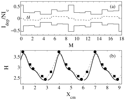
FIG. 10.: (a) Simulated depinning currents for $N=9$ ring with $\lambda_{j}=0.25$ and $h_{j-1}=1$, $h_{j}=0.5$, and $h_{j+1}=0.25$. Solid lines are the depinning current as current is increased or decreased while the dashed line is the difference of the up and down depinning current. (b) Numerically calculated pinning potential. Symbols are analytical calculation of the energy when a kink is in a plaquette (squares) and on a junction (circles). The actual kink position is calculated using Eq. (23). Dashed line is a guide to the eye.

There are three features in the depinning current vs. $M$ graph. First, the kink is traveling in a ratchet pinning potential. For $M=1$, as the current is swept in the positive direction the depinning current is different than when it is swept in the negative direction. Second, the depinning current has the expected odd inversion symmetry; that is $I_{dep+}(M)=I_{dep-}(T-M)$. Thirdly, the depinning current is periodic with period $T=9$. All these features were predicted by the theory developed above.

The observation that the kink is traveling in a ratchet pinning potential can be directly verified by calculating the pinning potential. We will use both the analysis described above and the numerical method used in [12], which allows us to compute the energy of the kink as it moves from a maximum to a minimum. The position of the kink in the array is calculated with

$$X_{cm}={1\over 2}+{1\over 2\pi}\sum_{j=1}^{N}j(\varphi_{j+1}-\varphi_{j}).$$ (23)

In Fig. 10(b) we have plotted the numerically calculated pinning potential. We place the kink on the energy maximum and perturb it along the unstable direction and calculate the energy using Eq. (15) and the kink position using Eq. (23). We have also superimposed the values of the kink pinning potential calculated from the above analysis. We have used the linearized results to calculate the phases and Eq. (15) to calculate the energy. The circles represent the energy when the kink is approximately on a junction while the squares are the energy when the kink is approximately in a plaquette center. We see that the pinning potential is indeed asymmetric and that the analysis agrees well with the numerical result.

V Summary

We have shown that an inhomogeneous parallel Josephson-junction array provides an ideal experimental system to study kink motion in different potentials. In particular, we have designed a ratchet potential in an array with a ring geometry. One way of designing a ratchet potential is by varying cell inductances and junction areas. We have verified experimentally and numerically that a kink, and even a train of kinks, requires a different amount of force to depin in positive and negative directions. One interesting result for the inhomogeneous rings is that the periodicity in $M$ of the system will depend only on the inductance ratios of consecutive cells. As a consequence, it is possible to design a small ring, e.g. $N=8$, such that one can distinguish between hundreds of states with different number of trapped kinks.

We have also shown that a ratchet kink potential can be obtained by using junctions with three different critical currents. In this case, the inductances of all cells are equal and the array has a period in $M$ equal to the number of junctions.

We expect to investigate a kink in our ratchet potential with an ac bias to show that there is a rectifying effect: the ac force leads to kink drift in a preferred direction. This Brownian rectifier has the added technical benefit that the dc voltage response is quantized [12]. This opens up the possibility of designing electronic detectors that can directly measure the amplitude (instead of just the frequency) of an applied signal very accurately.

The ideas studied in this paper can be extended to the study of vortex depinning, vortex motion and flux flow in ratchet 2D Josephson-junction arrays. We just need to design a 2D array with an appropriate combination of critical currents and cell areas in the direction of vortex motion, which is perpendicular to the current injection direction.

Another way of designing a ratchet effect is by controlling the critical current of the individual junctions of a regular homogeneous array with the application of an external magnetic field. In this way, we can make a physical realization of a “flashing ratchet”. The mechanics of motion is well understood [3, 5]. The pinning potential is removed periodically. In the interval in which the potential is off, particles can diffuse freely. After restoration of the pinning potential, most of the particles localize again in the minimum of the next lattice site giving a net motion (in the opposite direction of the “rocking ratchet”). However, as we have seen temperature (i.e., diffusion) does not play an important role in the motion of the kink. Nevertheless, one can devise a new mechanism for the kink motion in this context. After the removal of the pinning potential, kinks delocalize in an asymmetric way and localize again (when the pinning potential appears) in the next plaquette. Preliminary numerical simulations [22] confirm this scenario.

The study of inhomogeneous 1D arrays of Josephson junctions can also help to elucidate pinning mechanism in both 2D Josephson-junction arrays and superconducting thin films. Also, systems in which critical currents are modulated [23] can show complex and interesting dynamical behavior. In these systems and mainly in the presence of ac driving, we expect the appearance of new collective coherent vortex motion which can give a mode-locking response. Thus, these ratchet arrays may be used as inspiration for devices that take advantage of the properties of directional transport, rectification, and quantized response to ac driving.

An interesting application of directional motion of vortices has already been proposed in [7]. An appropriate ratchet potential (via the modulation of the thickness of the superconductor) is used to eliminate vortices from the thin film. This “cleaning” is also convenient in 1D and 2D Josephson-junction arrays in which the presence of trapped flux breaks the phase coherence of, for instance, arrays used as radiation sources or complex rapid single flux quantum (RSFQ) circuits. It appears that our ratchet pinning potential could be used to “clean” this trapped flux.

In summary, we have shown that inhomogeneous parallel arrays of Josephson arrays are ideal model systems for the study of flux pinning. We have also shown that there are different ways to build a ratchet pinning potential, and have found an excellent agreement between experiments and theory.

Appendix

In this appendix we calculate the periodicity in the number of kinks, $M$, of Eq. (6) for a general inhomogeneous ring array. Importantly, this period depends only on the ratio between consecutive $\lambda^{\prime}s$ and it is independent of the order of such ratios and the values of the critical currents.

As in the main text, we will use the following transformation for the phases:

$$\psi_{j}=\varphi_{j}+2\pi m_{j},$$ (24)

where $m_{j}$ is an integer. Eq. (9) is the new equation of motion in the new variables. The new boundary condition for the transformed variables becomes $\psi_{j+N}=\psi_{j}+2\pi(M+T)$ with $T=m_{j+N}-m_{j}$. The strategy to calculate the period $T$ will be to find a set of integers that eliminate the $m_{j}$ dependence in the right hand side of Eq. (9). We will look for solutions where $m_{j}-m_{j-1}+(m_{j}-m_{j+1})\lambda_{j}/\lambda_{j-1}=0$. Clearly, this condition is independent of $h_{j}$ and only depends on the ratios $\lambda_{j}/\lambda_{j-1}$.

First we let $\lambda_{j}/\lambda_{j-1}=p_{j}/q_{j}$ with $p_{j}$ and $q_{j}$ coprime. Since only differences of $m_{j}$ are needed, we let $m_{1}=0$ without loss of generality. Then we solve for $m_{3}$ in terms of $m_{2}$,

$$m_{3}={p_{2}+q_{2}\over p_{2}}m_{2}.$$ (25)

Similarly, $m_{4}$ in terms of $m_{3}$ is

$$m_{4}={q_{2}q_{3}+p_{3}(p_{2}+q_{2})\over p_{3}(p_{2}+q_{2})}m_{3}.$$ (26)

After some algebra we find the following recursive formula for $m_{j+1}/m_{j}$:

$$m_{j+1}/m_{j}=\xi_{j+1}/p_{j}\xi_{j},$$ (27)

with

$$\xi_{j}=\prod_{k=2}^{j-1}q_{k}+p_{j-1}\xi_{j-1}.$$ (28)

Here $\xi_{2}=1$ and $j=3$ to $N+1$. We have now derived that the ratio of $m_{j+1}/m_{j}$ is a ratio of integers. So in principle, we can find an integer for every $m_{j}$.

To find a set of integers for $m_{j}$ we start at the most complex ratio: $m_{N+1}/m_{N}$. We take $m_{N+1}=\xi_{N+1}$ and $m_{N}=p_{N}\xi_{N}$. By back substituting, we find

$$m_{j}=\xi_{j}\prod_{k=j}^{N}p_{k}$$ (29)

for $j=2$ to $N$ and with $m_{1}=0$.

It is straight forward to find the period. Since we have taken $m_{1}=0$ the period can be most easily expressed as $T=m_{N+1}$,

$$T={\prod_{k=2}^{N}q_{k}}+p_{N}\xi_{N}.$$ (30)

For consistency we also check that the equations at $j=1$ are satisfied: $m_{0}+m_{2}\lambda_{1}/\lambda_{N}=0$. It is relatively easy to find that $m_{0}=-\prod_{k=2}^{N}q_{k}$. The period calculated using $T=m_{N}-m_{0}$ also yields Eq. (30). This completes the existence prove that an inhomogeneous parallel array with consecutive $\lambda^{\prime}s$ that are rational numbers has a period in $M$.

This procedure, however, will not necessarily yield the minimum period. To calculate the minimum period we need to find the smallest $m_{N+1}$. For each ratio of $m_{j}$, we can make the numerator and denominator of $\xi_{j+1}/p_{j}\xi_{j}$ relatively prime by dividing by their common multiples. We start with the last ratio $m_{N+1}/m_{N}=\xi_{N+1}/p_{N}\xi_{N}$. If we let $y=\gcd(\xi_{N+1},p_{N}\xi_{N})$ then $m_{N+1}=\xi_{N+1}/y$ and $m_{N}=p_{j}\xi_{N}/y$. However, we also need to be able to consistently change $m_{N}$. That is, the ratio $m_{N}/m_{N-1}=p_{N}\xi_{N}/p_{N}p_{N-1}\xi_{N-1}$ should still be valid. This implies that $y$ has to be a multiple of $m_{N-1}$ as well. By iterating, we see that $y$ has to be a multiple of all the $m_{j}$. Therefore, let $x=\gcd(m_{N+1},m_{N},\ldots,m_{2})$. The minimum integer period is then

$$T=({\prod_{k=2}^{N}q_{k}}+p_{N}\xi_{N})/x.$$ (31)

As an example, let us consider the regular ring with $\lambda_{j}=\lambda$. Here $\xi_{N+1}=N,\gcd(N,N-1,N-2,\ldots,1)=1$ and $T=N$ as expected from the homogeneous sine-Gordon equation. This explains the observation in Fig. 10 that T=9.

As another example, we consider the ring with alternating areas. Let $\lambda_{j}/\lambda_{j-1}=p/q$ for $j$ even and $\lambda_{j}/\lambda_{j-1}=q/p$ for $j$ odd. Then $\xi_{3}=p+q$, $\xi_{4}=2pq+q^{2}$, and

$$\xi_{N}={N\over 2}p^{N/2-1}q^{{N/2}-1}+({N\over 2}-1)p^{N/2-2}q^{N/2}$$ (32)

for $N$ even. Also

$$\prod_{k=2}^{N}q_{k}=p^{N/2-1}q^{N/2}.$$ (33)

Then, $x=\gcd(m_{N+1},m_{N},\ldots,m_{2})=p^{N/2-1}q^{N/2-1}$ and

$$T = (N/2)p+(N/2-1)q+q$$ (34)

$$= (p+q)N/2.$$ (35)

We have recovered the same result derived in the main text.

REFERENCES

- [1] Y. Braiman, J. F. Lindner, and W. L. Ditto, Nature 378, 465 (1995).
- [2] P. Jung, Phys. Rep. 234, 175 (1994); L. Gammaitoni, P. Hänggi, P. Jung and F. Marchesoni, Rev. Mod. Phys. 70, 223 (1998).
- [3] R. D. Astumian, Science 276, 917 (1997); F. Jülicher, A. Ajdari, J. Prost, Rev. Mod. Phys. 69, 1269 (1997).
- [4] M. O. Magnasco, Phys. Rev. Lett. 71, 1477 (1993);
- [5] R. Bartussek, P. Hänggi, and J.G. Kissner Europhys. Lett., 28, 459 (1994); P. Hänggi and R. Bartussek in Nonlinear Physics of Complex Systems, Lectures Notes in Physics, Vol 476 (Springer, Berlin) 294-308 (1996).
- [6] J. Rousselet, L. Salome, A. Ajdari and J. Prost, Nature 370, 446 (1994).
- [7] C.S. Lee, B. Janko, I. Derényi and A.L. Barabasi, Nature 400, 337 (1999).
- [8] I. Derényi, Ch. Lee and A.L. Barabasi, Phys. Rev. Lett. 80, 1473 (1998).
- [9] See L. M. Floría and J. J. Mazo, Adv. Phys. 45, 505 (1996) and references therein.
- [10] A. V. Ustinov, M. Cirillo and B. A. Malomed, Phys. Rev. B 47, 8357 (1993); S. Watanabe, H. S. J. van der Zant, S. H. Strogatz and T. P. Orlando, Physica D 97, 429 (1996).
- [11] D. J. Resnick, J. C. Garland, J. T. Boyd, S. Shoemaker and R. S. Newrock, Phys. Rev. Lett. 47, 1542 (1981).
- [12] F. Falo, P. J. Martínez, J. J. Mazo, and S. Cilla, Europhys. Lett. 45, 700 (1999).
- [13] To derive the circuit equations we need to apply both Kirchhoff’s current law (KCL) at the nodes and Kirchhoff’s voltage law (KVL) for each loop. In circuits with Josephson junctions, KVL is superseded by the more stringent requirement of flux quantization. Flux quantization gives a constraint on the flux of a loop while KVL only constrains the derivative of the flux, i.e. the voltage. Satisfying flux quantization automatically satisfies KVL.
- [14] We have used the Josephson-voltage relation and set the damping () to . The damping is usually referred to as the Stewart-McCumber parameter .
- [15] In the case of an open array, where open boundary conditions must be imposed, , and otherwise.
- [16] There are several ways of calculating the periodicity in of the sine-Gordon equation (regular array). Probably the most straight forward is to find a transformation that moves the dependence from the boundary conditions to the sine term. In the case of the regular discrete sine-Gordon equation the new phases are just . Then appears only in and the periodicity of the equations in is just . Though this approach can also be used in an inhomogeneous rings, it is not trivial to guess the correct transformation.
- [17] Due to the convex (i.e. inductive) character of the inter-junction coupling all the junctions show the same dc IV curve.
- [18] V. Ambegaokar and A. Baratoff, Phys. Rev. Lett. 10, 486 (1963).
- [19] FastHenry, see http://rle-vlsi.mit.edu. See also E. Trías, Ph.D. thesis, Massachusetts Institute of Technology, 1999.
- [20] This correspond to a perturbative expansion from the so-called anti-integrable limit (), which can be rigorously justified (C. Baesens, private communication). For another example see S. Kim, C. Baesens and R. S. Mackay, Phys. Rev. E 56, 4955 (1997).
- [21] See, for example, P. Jung, J. G. Kissner and P. Hänggi Phys. Rev. Lett. 76, 3436 (1996), for underdamped effects in a ratchet potential.
- [22] Unpublished results.
- [23] F. Domínguez-Adame, A. Sánchez and Y.S Kivshar, Phys. Rev.E 52, 2183 (1995); E. Lennholm and M. Hornquist, Phys. Rev.E 59, 381 (1999).