Spin correlation functions and susceptibilities in the easy-plane XXZ chain

The study of low–dimensional spin systems constitutes a growing field of research which is mainly due to the availability of new materials, such as the quasi–one–dimensional (1D) cuprates [1]. Recently, an unexpected quantum–classical crossover of the longitudinal spin correlation functions in the 1D XXZ model

$${\cal H}=\frac{J}{2}\sum_{\langle i,j\rangle}(S_{i}^{+}S_{j}^{-}+\Delta S_{i}^{z}S_{j}^{z})$$ (1)

($\langle i,j\rangle$ denote nearest–neighbor (NN) sites along the chain; throughout we set $J=1$) was found for $-1<\Delta<0$ by means of exact diagonalization (ED) of systems up to 18 spins [2] and by the quantum transfer matrix formalism [3].

Motivated by those findings, in this paper we examine the spin correlation functions in the easy–plane region $-1<\Delta<1$ of the model (1) by an analytical approach based on a Green’s–function projection method. This theory was found to provide a good description of antiferromagnetic (AFM) short–range order (SRO) in the 2D spatially isotropic [4] and anisotropic Heisenberg models [5]. Moreover, for the first time, we calculate the full wavenumber, temperature and $\Delta$ dependences of the static transverse and longitudinal spin susceptibilities.

To determine the dynamic spin susceptibilities $\chi^{+-}(q,\omega)=-\langle\langle S_{q}^{+};S_{-q}^{-}\rangle\rangle_{\omega}$ and $\chi^{zz}(q,\omega)=-\langle\langle S_{q}^{z};S_{-q}^{z}\rangle\rangle_{\omega}$ $(-\pi\leq q\leq\pi)$, defined in terms of two–time retarded commutator Green’s functions, by the projection method, we choose the two-operator basis ${\bf A}_{1}=(S_{q}^{+},i\dot{S}_{q}^{+})^{T}$ and ${\bf A}_{2}=(S_{q}^{z},i\dot{S}_{q}^{z})^{T}$, respectively, and consider the matrix Green’s function $\langle\langle{\bf A};{\bf A}^{\dagger}\rangle\rangle_{\omega}$, neglecting the self–energy part [4], $\langle\langle{\bf A};{\bf A}^{\dagger}\rangle\rangle_{\omega}=[\omega-{\mathfrak{M}}^{\prime}{\mathfrak{M}}^{-1}]^{-1}{\mathfrak{M}}$ with ${\mathfrak{M}}=\langle[{\bf A},{\bf A}^{\dagger}]\rangle$ and ${\mathfrak{M}}^{\prime}=\langle[i\dot{\bf A},{\bf A}^{\dagger}]\rangle$. We get

$$\chi^{\nu}(q,\omega)=-\frac{M^{\nu(1)}_{q}}{\omega^{2}-(\omega_{q}^{\nu})^{2}}\,;\;\;\nu=+-,\,zz,$$ (2)

where the first spectral moments $M_{q}^{\nu(1)}$ are given by the exact expressions

$$M_{q}^{+-(1)} = -2[C_{1}^{+-}(1-\Delta\cos q)+2C_{1}^{zz}(\Delta-\cos q)]\,,$$ (3)

$$M_{q}^{zz(1)} = -2C_{1}^{+-}(1-\cos q)\,.$$ (4)

The two–spin correlation functions $C_{n}^{+-}=\langle S_{0}^{+}S_{n}^{-}\rangle$ and $C_{n}^{zz}=\langle S_{0}^{z}S_{n}^{z}\rangle$ are calculated from

$$C_{n}^{\nu}=\frac{1}{N}\sum_{q}\frac{M_{q}^{\nu(1)}}{2\omega_{q}^{\nu}}[1+2p(\omega_{q}^{\nu})]\mbox{e}^{iqn}\,,$$ (5)

where the Bose function $p(\omega_{q}^{\nu})=(\mbox{e}^{\omega_{q}^{\nu}/T}-1)^{-1}$ appears due to the use of commutator Green’s functions. The NN correlation functions are directly related to the internal energy per site $\varepsilon=C_{1}^{+-}+\Delta C_{1}^{zz}$.

To obtain the spectra $\omega_{q}^{\nu}$ in the approximations $-\ddot{S}^{+}_{q}=(\omega_{q}^{+-})^{2}S^{+}_{q}$ and $-\ddot{S}^{z}_{q}=(\omega_{q}^{zz})^{2}S^{z}_{q}$, we take the site-representation and decouple the products of three spin operators in $-\ddot{S}^{+}_{i}$ and $-\ddot{S}^{z}_{i}$ along the NN sequence $\langle i,j,l\rangle$ introducing vertex parameters in the spirit of the scheme proposed by Shimahara and Takada [6],

$$S_{i}^{+}S_{j}^{+}S_{l}^{-} = \alpha^{+-}_{1}\langle S_{j}^{+}S_{l}^{-}\rangle S_{i}^{+}+\alpha_{2}^{+-}\langle S_{i}^{+}S_{l}^{-}\rangle S_{j}^{+}\,,$$ (6)

$$S_{i}^{z}S_{j}^{+}S_{l}^{-} = \alpha^{zz}_{1}\langle S_{j}^{+}S_{l}^{-}\rangle S_{i}^{z}\,,$$ (7)

$$S_{i}^{+}S_{j}^{z}S_{l}^{-} = \alpha^{zz}_{2}\langle S_{i}^{+}S_{l}^{-}\rangle S_{j}^{z}\,.$$ (8)

Here, $\alpha_{1}^{\nu}$ and $\alpha_{2}^{\nu}$ appearing in $\omega_{q}^{\nu}$ are attached to correlation functions between nearest and further-distant neighbors functions, respectively. We obtain

$$(\omega_{q}^{+-})^{2} = \frac{1}{2}[(1+2\alpha_{2}^{+-}C_{2}^{+-})(1-\Delta\cos q)$$ (12)

$$\;\;+\Delta(1+4\alpha_{2}^{+-}C_{2}^{zz})(\Delta-\cos q)$$

$$\;\;+2\alpha_{1}^{+-}C_{1}^{+-}(\Delta\cos 2q-\cos q)$$

$$\;\;+4\alpha_{1}^{+-}C_{1}^{zz}(\cos 2q-\Delta\cos q)]\,,$$

$$(\omega_{q}^{zz})^{2} = (1-\cos q)[1+2\alpha_{2}^{zz}C_{2}^{+-}$$ (14)

$$\;\;-2\Delta\alpha_{1}^{zz}C_{1}^{+-}(1+2\cos q)]\,.$$

In the easy-plane region $-1<\Delta<1$, the theory has eight quantities to be determined self-consistently ($C_{1}^{\nu}$, $C_{2}^{\nu}$, $\alpha_{1}^{\nu}$, $\alpha_{2}^{\nu}$) and six self-consistency equations (5) including the sum rules $C_{0}^{+-}=1/2$ and $C_{0}^{zz}=1/4$. To get the two remaining conditions for determining the free $\alpha$-parameters $\alpha_{2}^{\nu}$ we may adopt different phenomenological choices. Following the approach by Kondo and Yamajii [7] for the isotropic Heisenberg chain ($\Delta=1$; $\alpha_{i}^{+-}=\alpha_{i}^{zz}$), let us first consider the simple conditions $\alpha_{2}^{\nu}=\alpha_{1}^{\nu}$. In this case we do not obtain quantitatively satisfactory results (cf. Fig. 1); therefore, we improve the theory by another choice with $\alpha_{2}^{\nu}\neq\alpha_{1}^{\nu}$. For it we need additional conditions. At $T=0$, it is natural to adjust $\alpha_{2}^{\nu}$ to $C_{1}^{\nu}$ taken from the exact expressions for the ground-state energy $\varepsilon(\Delta)$ [8] and the NN correlator $C_{1}^{zz}$ [9] (see Fig. 1). Moreover, to formulate conditions also at finite temperatures, we follow the reasonings of Ref. [6] and [4] and conjecture that both “vertex corrections” $\alpha_{1}^{\nu}(T)-1$ and $\alpha_{2}^{\nu}(T)-1$ have similar temperature dependences and vanish in the high-temperature limit. Correspondingly, as the simplest interpolation between high temperatures and $T=0$ we assume the ratio $R$ of two vertex corrections as temperature independent and given by the ground-state value. To be specific, in calculating $\chi^{zz}(q,\omega;T)$ for all $\Delta$, we assume

$$\frac{\alpha_{2}^{zz}(T)-1}{\alpha_{1}^{zz}(T)-1}=R^{zz}\,.$$ (15)

For $\chi^{+-}(q,\omega;T)$ the additional condition analogous to Eq. (15) (substitution of $\alpha_{i}^{zz}$ by $\alpha_{i}^{+-}$) yields a solution of the self-consistency equations only in the case $\Delta>0$. For $\Delta<0$ it turns out that a solution can be obtained using a slightly modified condition (substitution of $\alpha_{2}^{zz}$ in Eq. (15) by $\alpha_{2}^{+-}$). That is, for $\chi^{+-}(q,\omega;T)$ we require

$$\frac{\alpha_{2}^{+-}(T)-1}{\alpha_{1}^{+-}(T)-1} = R_{>}^{+-}\,,$$ (16)

$$\frac{\alpha_{2}^{+-}(T)-1}{\alpha_{1}^{zz}(T)-1} = R_{<}^{+-}\,.$$ (17)

The set of self-consistency equations is solved numerically by Broyden’s method with relative error less than 10^-7.

To discuss the rotational invariance of the theory at $\Delta=\pm 1$, it is useful to perform the unitary transformation which rotates the spins on all odd sites $m=2l+1$ around the $z$-axis by the angle $\pi$ [10]. Taking the unitary operator $U=\prod_{m}2S_{m}^{z}$ which transforms ${\bf S}_{n}$ as $\tilde{\bf S}_{n}=U^{+}{\bf S}_{n}U$, we get

$$\tilde{S}_{n}^{x,y}=\mbox{e}^{i\pi n}S_{n}^{x,y}\,,\;\tilde{S}_{n}^{z}=S_{n}^{z}\,,\\$$ (18)

and

$$\tilde{H}=\frac{1}{2}\sum_{\langle i,j\rangle}(-S_{i}^{+}S_{j}^{-}+\Delta S_{i}^{z}S_{j}^{z})\,.$$ (19)

Since $\langle A\rangle_{\cal H}=\langle\tilde{A}\rangle_{\tilde{\cal H}}$ for any operator $A$, by (18) we obtain the relation

$$\chi^{+-}_{\cal H}(q,\omega)=\chi_{\tilde{\cal H}}^{+-}(k,\omega)\,;\;\;k=q-\pi\,,$$ (20)

and $\chi^{zz}_{\cal H}(q,\omega)=\chi_{\tilde{\cal H}}^{zz}(q,\omega)$. For the correlation functions we have $C^{+-}_{n,\cal H}=\mbox{e}^{i\pi n}C^{+-}_{n,\tilde{\cal H}}$ and $C^{zz}_{n,\cal H}=C^{zz}_{n,\tilde{\cal H}}$. Evidently, for $\Delta=1$ the rotational symmetry is preserved, i.e., $C_{n}^{+-}=2C_{n}^{zz}$, $\alpha_{i}^{+-}=\alpha_{i}^{zz}$, $\omega_{q}^{+-}=\omega_{q}^{zz}$, and $\chi^{+-}(q,\omega)=2\chi^{zz}(q,\omega)$. At $\Delta=-1$, the rotational symmetry occurs in the transformed model (19), where the relations $\chi_{\tilde{\cal H}}^{+-}(q,\omega)=\chi^{+-}_{\cal H}(q+\pi,\omega)=2\chi_{\tilde{\cal H}}^{zz}(q,\omega)$ and $2C^{zz}_{n,\tilde{\cal H}}=C^{+-}_{n,\tilde{\cal H}}$ can be easily verified from Eqs. (3), (4), (12), and (14).

Corresponding to the unitary equivalence of $\tilde{\cal H}$ and ${\cal H}$ we denote the (paramagnetic) easy-plane region with $-1<\Delta<0$ as ferromagnetic (FM) region (cf. Eq. (19)) and the region with $0<\Delta<1$ as AFM region (cf. Eq. (1)).

Concerning the question of magnetic long-range order (LRO), in the easy-plane XXZ chain there is no LRO which is correctly reproduced by our theory. In Ref. [5] the description of LRO within our scheme (mode condensation) is outlined for the spatially anisotropic Heisenberg model, and the absence of LRO in the 1D limit is shown. Considering the model (1) at $|\Delta|<1$ and allowing for a possible finite condensation part $C$ in the spin correlators [5], a solution of our self-consistency equations only exists for $C=0$, i.e., there is no LRO.

In Fig. 1 the zero-temperature correlators appearing in the spectra (12) and (14) are plotted as functions of $\Delta$. The NN correlators $C_{1}^{\nu}$, in particular $C_{1}^{zz}$, calculated by the simplified theory ($\alpha_{2}^{\nu}=\alpha_{1}^{\nu}$) strongly deviate from the exact values [8, 9], especially in the vicinity of $\Delta=0$. The same refers to $\chi^{zz}(0)$. Therefore, in the following we only show and discuss the results obtained by the improved theory [cf. Eqs. (15) to (17).] At $\Delta=1$ the rotational symmetry is visible. At the quantum critical point $\Delta=-1$ there occurs FM LRO [10], and a non-analytical behavior is observed, e.g., $\lim_{\Delta\to-1^{+}}\partial C_{1}^{zz}/\partial\Delta=\infty$ and $\lim_{\Delta\to-1^{-}}\partial C_{1}^{zz}/\partial\Delta=0$ [8]. Moreover, at $\Delta=-1$, we have $C^{+-}_{n,\tilde{\cal H}}=1/6$. This limiting behavior, however, is hard to obtain numerically because of the infinite slope of $C^{\nu}_{n}$ as $\Delta\to-1^{+}$.

Figure 2 displays the static susceptibilities $\chi^{\nu}(q=0,\pi)$ at $T=0$ vs. $\Delta$. First let us emphasize the excellent agreement of our result for the longitudinal uniform susceptibility with the exact result [11] over the whole $\Delta$ region (cf. inset), where $\chi^{zz}(0)$ varies by two orders of magnitude. That means, the longitudinal spin correlations of arbitrary range are well described by our theory. In the FM region, the uniform longitudinal susceptibility diverges in the limit $\Delta\to-1$ (cf. Fig. 5 (a)) indicating the instability of the paramagnetic phase against the FM LRO phase at $\Delta=-1$ [12]. The same is true for the staggered transverse susceptibility $\chi^{+-}_{\cal H}(\pi)$ (cf. Fig. 5 (b)) which, by Eq. (20), is equivalent to the uniform transverse susceptibility $\chi^{+-}_{\tilde{\cal H}}(0)$.

The wavenumber dependences of the zero-temperature static susceptibilities $\chi^{\nu}(q)$ are depicted in Fig. 3. For sufficiently low values of $\Delta$ in the FM region, $\chi^{zz}(q)$ shows a maximum at $q=0$ being indicative of the FM instability (cf. Fig. 2). Accordingly $\chi^{+-}_{\cal H}(q)$ has a maximum at $q=\pi$ (Fig. 3 (b)) corresponding, by Eq. (20), to the maximum of $\chi^{+-}_{\tilde{\cal H}}(k)$ at $k=0$. In the AFM region, the longitudinal and transverse susceptibilities reveal peaks at the AFM wavenumber being indicative of the AFM LRO at $\Delta>1$.

Let us now discuss the finite-temperature behavior of the longitudinal spin correlation functions. Table I shows that in the AFM region we get the expected alternating signs of $C_{n}^{zz}$ being characteristic of AFM SRO. By contrast, in the FM region, $C_{n}^{zz}<0$ holds $\forall n$ below some characteristic temperature $T_{0}(\Delta)$ [2]. In view of the approximations made in our theory, the analytical results obtained for $C_{n}^{zz}$ are in reasonable agreement with the exact data for the 18-site chain. At fixed separation $n$ and with increasing temperature or above $T_{0}(\Delta)$ with increasing separation, $C_{n}^{zz}$ changes sign from negative to positive values. This property can be interpreted as a quantum-classical crossover [2] because with increasing temperature the system behaves more classically, i.e., it becomes dominated by the potential energy (longitudinal part of the Hamiltonian). It is worth emphasizing that the so-called “sign changing effect” in the longitudinal spin correlations found numerically [2] is reproduced for the first time by an analytical theory. This is demonstrated in Table II. The temperatures $T_{0}(n,\Delta)$ where $C_{n}^{zz}(T_{0}(n,\Delta),\Delta)=0$ are compared with the ED results showing an increasing agreement with decreasing anisotropy parameter $\Delta$. As might be expected, for the 2D XXZ model our results for $T_{0}({\bf r},\Delta)$ much better agree with the exact data (cf. Table II). A detailed study of the 2D case is presented in Ref. [13].

Figure 4 shows the temperature dependence of the transverse correlation functions in the FM region. The oscillating behavior of $C_{n}^{+-}(T)$ (sign $(-1)^{n}$) and the decrease of $|C_{n}^{+-}|$ with increasing separation $n$ (at fixed temperature) and increasing temperature (at fixed $n$) indicates a transverse AFM SRO (but no LRO) related to the maximum of $\chi_{\cal H}^{+-}(q)$ at $q=\pi$ (cf. Fig. 3 (b)). However, due to the equality $C_{n,\cal H}^{+-}=(-1)^{n}C_{n,\tilde{\cal H}}^{+-}$, for $\Delta<0$ we prefer to denote this SRO more physically as transverse FM SRO (in the model $\tilde{\cal H}$), where $C_{n,\tilde{\cal H}}^{+-}(T)$ can be read off immediately from Fig. 4. Accordingly, for $\Delta>0$, we get transverse AFM SRO (similar behavior of $C_{n}^{+-}(T)$ as shown in Fig. 4).

In Fig. 5 various susceptibilities $\chi^{\nu}(q)$ at $q=0,\,\pi$ are plotted as functions of temperature. At $T=0$, the divergences of $\chi_{\cal H}^{zz}(0)$ and $\chi_{\cal H}^{+-}(\pi)=\chi_{\tilde{\cal H}}^{+-}(0)$ in the limit $\Delta\to-1$, discussed above (Fig. 2), are clearly seen. In the region $-0.3<\Delta<0$ the uniform longitudinal susceptibility reveals a maximum at $T_{max}$ which may be explained as follows. For $T<T_{0}(\Delta,n)$ the longitudinal SRO, characterized by $C_{n}^{zz}<0$ (cf. Table I), leads to a spin stiffness against the orientation of the spins along a homogeneous external field in $z$-direction so that $\chi^{zz}(0)$ is suppressed. With increasing temperature the correlations become increasingly ferromagnetic, which results in an increase of $\chi^{zz}(0;T)$ up to $T_{max}$ determined by $T_{0}(n,\Delta)$. With decreasing $\Delta$ $(-1<\Delta<-0.3)$ the maximum disappears, since the spin correlations are predominantly ferromagnetic. Thus, the maximum in $\chi^{zz}(0;T)$ for $-0.3<\Delta<0$ may be understood as a combined SRO and sign changing effect. In the AFM region, the maximum in the longitudinal susceptibility (see Fig. 5 (a)) obtained at all $\Delta$, where $T_{max}$ shifts to higher values with increasing $\Delta$, is due to the decrease of AFM SRO with increasing temperature. At large enough values of $\Delta$, besides the maximum in $\chi^{zz}(0;T)$ there appears a minimum at a finite temperature which was also found for the isotropic Heisenberg chain [7] and contradicts the exact behavior [14]. Note that this artifact does not occur in the 2D XXZ model [13]. In the high-temperature limit, all susceptibilities depicted in Fig. 5 reveal a crossover to the Curie-Weiss behavior.

Finally, in Fig. 6 the temperature dependence of the susceptibility $\chi_{\cal H}^{+-}(0)=\chi_{\tilde{\cal H}}^{+-}(\pi)$ is shown which again may be explained as SRO effect. Here, in the FM region, the transverse FM SRO results in a spin stiffness against the orientation of the transverse spin components along a staggered external field perpendicular to the $z$-direction so that $\chi_{\tilde{\cal H}}^{+-}(\pi)$ is suppressed at low temperatures and exhibits a maximum. In the AFM region, the transverse AFM SRO results in an analogous temperature dependence of $\chi_{\cal H}^{+-}(0;T)$, where in the whole easy-plane region $T_{max}$ increases with increasing $\Delta$.

To summarize, we presented a Green’s-function theory of magnetic SRO in the 1D easy-plane XXZ model which allows, for the first time, the calculation of all static magnetic properties over the whole easy-plane FM and AFM regions, where no LRO occurs. That is, we computed the full wavenumber and temperature dependences of the anisotropic static spin susceptibilities and of the spin correlation functions of arbitrary range and at arbitrary temperature. In particular, in the FM region, we are able to reproduce the quantum-classical crossover in the longitudinal spin correlations in qualitative agreement with the numerical diagonalization data of Ref. [2]. Moreover, the obtained maxima in the temperature dependences of the uniform longitudinal and transverse susceptibilities are explained as SRO effects. From the results of our theory we conclude that this approach may be successfully applied to other anisotropic spin models, where the description of spin correlations improves in higher dimensions [13].

The authors would like to thank Y. Gaididei, J. Stolze, and A. Weiße for helpful discussions.

Figure Captions

Fig. 1. Transverse and longitudinal spin correlation functions $C_{n}^{\nu}$ ($n=1,2$) at $T=0$.

Fig. 2. Zero-temperature static susceptibilities at $q=0,\,\pi$.

Fig. 3. Wavenumber dependence of the longitudinal (a) and transverse (b) static susceptibilities at $T=0$.

Fig. 4. Transverse correlation functions up to the fourth-nearest neighbors in the easy-plane ferromagnetic region.

Fig. 5. Inverse uniform longitudinal (a) and staggered transverse susceptibility (b).

Fig. 6. Temperature dependence of the uniform transverse susceptibility.

TABLE I.: Longitudinal spin correlation functions $C_{n}^{zz}(T;\Delta)$ for the easy-plane XXZ chain with $\Delta=\pm 0.3$ at $T=0.1$. The ED data given in parenthesis are taken from Ref. [2].

$\;\Delta$	$n=1$	$n=2$	$n=3$	$n=4$
$\;\;0.3$	$-1.15\times 10^{-01}$	$1.24\times 10^{-02}$	$-9.60\times 10^{-03}$	$1.34\times 10^{-04}$
$-0.3$	$-8.06\;[-8.38]\times 10^{-02}$	$-1.31\;[-1.29]\times 10^{-02}$	$-4.57\;[-8.08]\times 10^{-03}$	$-1.89\;[-2.70]\times 10^{-03}$

TABLE II.: Temperature $T_{0}(\Delta;{\bf r})$ of the sign change in the longitudinal correlation functions $C^{zz}_{\bf r}(T;\Delta)$ of the ferromagnetic easy-plane XXZ model. The corresponding results obtained from ED of a 18-site 1D chain [2] and a 2D 4$\times$4 square lattice with periodic boundary conditions are given in parenthesis.

$\Delta$	$T_{0}(\Delta;{\bf r})$
	1D case				2D case
	$n=1$	$n=2$	$n=3$	$n=4$	${\bf r}=(1,0)$	${\bf r}=(1,1)$	${\bf r}=(2,0)$
-0.1	3.10 [4.966]	2.18 [3.323]	1.72 [2.561]	1.12 [2.073]	2.98 [2.540]	1.76	1.76 [1.520]
-0.3	0.86 [1.561]	0.56 [1.071]	0.44 [0.839]	0.38 [0.687]	0.96 [0.931]	0.74	0.72 [0.713]
-0.7	0.28 [0.413]	0.20 [0.318]	0.14 [0.264]	0.12 [0.227]	0.46 [0.391]	0.36 [0.303]	0.34 [0.301]
-0.9	0.12 [0.137]	0.08 [0.118]	0.06 [0.104]	0.04 [0.092]	$<$0.2 [0.125]	$<$0.2 [0.106]	$<$0.2 [0.106]

FIG. 1.:

FIG. 2.:

FIG. 3.:

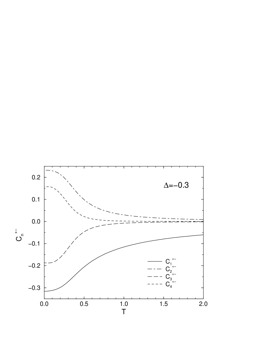
FIG. 4.:

FIG. 5.:

FIG. 6.:

REFERENCES

- [1] D. C. Johnston, in K. H. J. Buschow, editor, Handbook of Magnetic Materials, volume 10, Elsevier Science, (Amsterdam 1997); A. Tsvelik, Quantum Field Theory in Condensed Matter, Cambridge University Press, (Cambridge 1995).
- [2] K. Fabricius and B. M. McCoy, Phys. Rev. B 59, 381 (1999).
- [3] K. Fabricius, A. Klümper, and B. M. McCoy, Phys. Rev. Lett. 82, 5365 (1999).
- [4] S. Winterfeldt and D. Ihle, Phys. Rev. B 56, 5535 (1997).
- [5] D. Ihle, C. Schindelin, A. Weiße, and H. Fehske, Phys. Rev. B 60, 9240 (1999).
- [6] H. Shimahara and S. Takada, J. Phys. Soc. Jpn. 60, 2394 (1991); ibid. 61, 989 (1992).
- [7] J. Kondo and K. Yamaji, Prog. Theor. Phys. 47, 807 (1972).
- [8] C. N. Yang and C. P. Yang, Phys. Rev. 150, 321 (1966); ibid. 327 (1966);
- [9] J. D. Johnson, S. Krinsky, and B. M. McCoy, Phys. Rev. A 8, 2526 (1973).
- [10] Yu. A. Izyumov and Yu. N. Skryabin, Statistical Mechanics of Magnetically Ordered Ssystems, Consultants Bureau, (New York 1988).
- [11] M. Takahashi, Thermodynamics of one-dimensional solvable models, Cambridge University Press (Cambridge 1999).
- [12] Note that for a condensation part will occur within our scheme [5, 6].
- [13] H. Fehske, C. Schindelin, A. Weiße, H. Büttner, and D. Ihle, cond-mat/0006272
- [14] J. C. Bonner and M. E. Fisher, Phys. Rev. 135, A640 (1964); S. Eggert, I. Affleck, and M. Takahashi, Phys. Rev. Lett. 73, 332 (1994).