New Evidence of Earthquake Precursory Phenomena
in the 17 Jan. 1995 Kobe Earthquake, Japan

Abstract

Significant advances, both in the theoretical understanding of rupture processes in heterogeneous media and in the methodology for characterizing critical behavior, allows us to reanalyze the evidence for criticality and especially log-periodicity in the previously reported chemical anomalies that preceded the Kobe earthquake. The ion ($Cl^{-}$, $K^{+}$, $Mg^{++}$, $NO_{3}^{-}$ and $SO_{4}^{--}$) concentrations of ground-water issued from deep wells located near the epicenter of the 1995 Kobe earthquake are taken as proxies for the cumulative damage preceding the earthquake. Using both a parametric and non-parametric analysis, the five data sets are compared extensively to synthetic time series. The null-hypothesis that the patterns documented on these times series result from noise decorating a simple power law is rejected with a very high confidence level.

Since the inception of seismology, the search for reliable precursory phenomena of earthquakes has shown that the seismic process is preceded by a complex set of physical precursors. In addition to the direct seismic foreshocks [1, 2] and seismic precursors [3, 4], many other anomalous variations of various geophysical variables such as electric and magnetic fields and conductivity [5, 6], as well as chemical concentration [7, 8] have been documented. However, there is no consensus on the statistical significance of these precursors and their reliability [9, 10], due to a lack of reproducibility and of understanding of the underlying physical mechanisms.

One of the most striking reported seismic precursory phenomena are the time dependence of ion concentrations of ground-water issuing from deep wells located near the epicenter[7] and the ground water radon anomaly [8] preceding the earthquake of magnitude $6.9$ near Kobe, Japan, on January 17, 1995. Since the first quantitative analysis of this data, which suggested a discrete scale-invariant time-to-failure behavior [11], significant advances, both in the theoretical understanding of rupture processes in heterogeneous media and in the methodology needed to characterize critical behavior, permits a reassessment of the data.

Within the critical earthquake model [12, 4], a large earthquake is viewed as the culmination of a cooperative organization of the stress and of the damage of the crust in a large area extending over distances several times the size of the seismic rupture [3]. Most of the recently developed mechanical models [13, 14, 15, 16, 17] and experiments [18, 19] on rupture in strongly heterogeneous media (which is the relevant regime for the application to the earth) view rupture as a singular ‘critical’ point [20]: the cumulative damage $D$, which can be measured by acoustic emissions, by the total number of broken bonds or by the total surface of new rupture cracks, exhibits a diverging rate as the critical stress $\sigma_{c}$ is approached, such that $D$ can be written as an ‘integrated susceptibility’

$$D\approx A+B(\sigma_{c}-\sigma)^{z}~{},$$ (1)

The critical exponent $0<z<1$ is equal to $1/2$ in mean field theory [21, 16] and can vary depending on, e.g., the coupling corrosion and healing processes. In addition, it has been shown [18, 22, 23] that log-periodic corrections decorate the leading power law behavior (1), as a result of intermittent amplification processes during the rupture. They have also been suggested for seismic precursors [12]. This log-periodicity introduces a hierarchy of characteristic time and length scales with a prefered scaling ratio $\lambda$ [24]. As a result, expression (1) is modified into

$$D\approx A+B\left(\sigma_{c}-\sigma\right)^{z}+C\left(\sigma_{c}-\sigma\right)^{z}\cos\left(2\pi f\ln\left(\sigma_{c}-\sigma\right)+\phi\right)~{},$$ (2)

where $f=1/\ln(\lambda)$. Empirical [18], numerical [22, 23] as well as theoretical analyses [24] point to a prefered value $\lambda\approx 2.4\pm 0.4$, corresponding to a frequency $f\approx 1.2\pm 0.25$ or radial frequency $\omega=2\pi f\approx 7.5\pm 1.5$. A value for $\lambda$ close to $2$ is suggested on general grounds from a mean field calculation for an Ising and, more generally, a Potts model on a hierarchical lattice in the limit of an infinite number of neighbors [24]. It also derives from the mechanisms of a cascade of instabilities in competing sub-critical crack growth [22]. Empirically, we see that there is not rarely a bias towards a value twice this, corresponding to a better of signal-to-noise ratio for rescalings of $\lambda^{2}$ in the underlying renormalization group equation

The physical model underlying our analysis posits that the measured ion ($Cl^{-}$, $K^{+}$, $Mg^{++}$, $NO_{3}^{-}$ and $SO_{4}^{--}$) concentrations of ground-water issued from deep wells located near the epicenter of the 1995 Kobe earthquake are proxies for the cumulative damage preceding the earthquake. In this reaction-limited model, any fresh rock-water interface created by the increasing damage leads to the dissolution of ions in the carrying fluid that can be detected in the wells. We thus expect that the time evolution of measured ion concentration should follow closely the equation (2). Due to the large heterogeneity of rocks, this ‘deterministic’ signal should be decorated by noise with different realizations for each ion originating from different rock types. To test our hypothesis, we analyze the five ion data sets, thus increasing the statistical significance over our previous report [11]. However, it is possible that their noise realizations are not completely independent as some of the anions and cations are necessarily coupled pairwise. As we shall see, the poor result obtained from the analysis of $K^{+}$ might be due to the fact that it is generally coupled to both $Cl^{-}$ and $NO_{3}^{-}$.

Figure 1 shows the five data sets on which a moving average using three points has been applied. In this moving average, the middle point as usual carries double weight except for the two endpoints. Each of the five data sets is fitted with equation (2). The time intervals used in the fit were determined consistently for all five data sets by identifying the date of the lowest value of the concentration and using that date as the first data point. The last data point was taken as the last measurement before the earthquake. This gave $53$ points for the first three data sets, 52 for the fourth and 58 points for the fifth data set. For three of the data sets ($Cl^{-}$, $K^{+}$, and $NO_{3}^{-}$), the fit shown is also the best fit. In the case of $SO_{4}^{--}$, the best fit had an angular log-frequency $\omega\approx 19$ well above the expected range $6\leq\omega\leq 9$, while the second best fit has $\omega\approx 7$ within the expected range and is shown instead. This is also the case for $Mg^{++}$, where the best fit has a very low angular log-frequency $\omega\approx 2$ which capture nothing but a slowly varying trend. Here, the angular log-frequency of the second best fit $\omega\approx 16$ is approximately double of what is found for the other four data sets corresponding to a squaring of $\lambda$ as previously discussed. We note that the ranking of the fits is done using the variance between the data and the fit with equation (2), where the stress $\sigma$ has been replaced with time $t$, $t_{c}$ being the critical date of the earthquake. This assumes a Gaussian white noise-distribution, which constitutes a reasonable null-hypothesis for the noise but presumably does not fully reflect the reality.

Figure 1: The concentrations of $Cl^{-}$ (top left), $K^{+}$ (top right), $Mg^{++}$ (middle left), $NO_{3}^{-}$ (middle right) and $SO_{4}^{--}$ (lower left) as a function of date. The fit is equation (2). The values of the fits are $Cl^{-}$ : $A\approx 15.3$, $B\approx-1.9$, $C\approx 0.34$, $z\approx 0.58$, $t_{c}\approx 95.060$, $\phi\approx-0.40$ and $\omega\approx 7.0$. $K^{+}$: $A\approx 0.31$, $B\approx-.044$, $C\approx 0.036$, $z\approx 1.2$, $t_{c}\approx 95.061$, $\phi\approx 0.05$ and $\omega\approx 7.2$. $Mg^{++}$: $A\approx 5.5$, $B\approx-0.65$, $C\approx 0.11$, $z\approx 0.82$, $t_{c}\approx 95.069$, $\phi\approx-1.3$ and $\omega\approx 16$. $NO_{3}^{-}$: $A\approx 11.6$, $B\approx-3.7$, $C\approx-0.67$, $z\approx 0.28$, $t_{c}\approx 95.059$, $\phi\approx 2.1$ and $\omega\approx 7.5$. $SO_{4}^{--}$: $A\approx 17.3$, $B\approx-2.2$, $C\approx 0.83$, $z\approx 0.77$, $t_{c}\approx 95.066$, $\phi\approx-.31$ and $\omega\approx 7.4$.

Lower right figure is the Lomb periodogram of the five time series as a function of log-frequency defined as the conjugate to $\log\left(\left(t_{c}-t\right)/t_{c}\right)$. Prior to the spectral analysis, the leading power law has been removed using equation (3). The values of the Lomb peaks are  11,  3,  6,  13 and  5 in the same order as above.

We observe that the values of the critical time $t_{c}$ predicted for the earthquake from the various fits are not only very stable but also remarkably consistent with the true date $95.053$ of the earthquake. And except for the case of $Mg^{++}$, where it has approximately doubled, the same is true for the angular log-frequency $\omega$ (although in 2 cases, we took the second best fit as explained above). This robustness with respect to the date of the earthquake and the preferred scale ratio $\lambda=e^{2\pi/\omega}\approx 2.5$ is quite remarkable, considering that the value obtained for the exponent $z$ varies by approximately a factor of $4$ from the smallest to the largest value.

We complement these fits by a direct ‘non-parametric’ analysis of the log-periodic component, taken as a crucial test of the critical earthquake model captured by (1), (2). After de-trending each of the five chemical time series $c(t)$ using

$$c\left(t\right)\rightarrow\frac{c\left(t\right)-\left[A+B(t_{c}-t)^{z}\right]}{C(t_{c}-t)^{z}}~{},$$ (3)

which should leave a pure log-periodic cosine if no other effects were present, we apply a Lomb periodogram [25] to the de-trended data as a function of $\log\left(\left(t_{c}-t\right)/t_{c}\right)$. Lower fight figure of 1 shows the five spectra superimposed. In all case except for $K^{+}$, we observe significant peaks with a log-frequency $f\equiv{\omega\over 2\pi}$ between $1$ and $2$, i.e. $\omega$ is approximately between $6$ and $12.5$, and in two cases ($Cl^{-}$ and $NO_{3}^{-}$), we have two very clear peaks at $f\approx 1.2$ ($\omega\approx 7.5$) standing out with a Lomb weight of $\approx 11$ and $\approx 13$, respectively, in agreement with our prediction.

In order to assess the significance of these results, we present rather exhaustive statistical tests performed by constructing synthetic time series that differ from the real data only by the log-periodic pattern and we of course follow the same testing procedure.

There are several reasons why the results from the analysis above should be compared with those of synthetic tests. In particular, the real time series have been sampled non-uniformly in time because the water from the wells was collected from commercial bottles of which the production dates could be identified. We observe that the depletion process of bottles in stores implies that the number of bottles with a production date $t$ prior to the date of the earthquake $t_{c}$ is proportional to $\log\left(t_{c}-t\right)$, leading to a uniform sampling in $\log\left(t_{c}-t\right)$ instead of time $t_{c}-t$ to the earthquake. In order to investigate the effect of this sampling of the Kobe data with respect to log-periodic signatures, we have as a first step generated twenty synthetic data sets each with $56$ points as in the original data analyzed in ref.[11]. The synthetic data was generated using a noisy power law with the parameter values of the leading power law of the fit presented in ref.[11]. Specifically, the equation $c\left(t_{i}\right)=15.45+\left(-1.877+k\cdot\left(0.5-\mbox{ran}\right)\right)\cdot\left(95.053-t_{i}\right)^{0.44}$ was used with different noise-levels $k$. Here, ran is a uniform random number generator with values in the interval $\left[0:1\right[$ from [26]. In order to obtain a sampling similar to the one found in the original data, the sampling times $t_{i}$ of the synthetic data was chosen as $t_{i}=95.053-(95.053-93.847)e^{-5\mbox{ran}}$, where $93.847$ was the date of the first point in the original analysis. This then gives us a distribution of sampling times, which are uniform in log-time to $t_{c}$, where $t_{c}=95.053$ is the time at which the Kobe earthquake occurred. As noise-level, we used $k=0$, $k=0.37$ and $k=0.73$, corresponding to no-noise, a noise level of the same amplitude as the estimated log-periodic oscillations and a noise level twice that.

In the case of no noise $k=0$, the Lomb Periodograms exhibit in general a forest of peaks over a large log-frequency interval which average out to give a flat spectrum. Adding noise of amplitude $k=0.37$ and $k=0.73$ enhances the peaks but the averaging over the periodograms of the different synthetic data sets again produces an essentially flat spectrum. By “flat”, we mean that, in each individual synthetic time series, about $7$ “peaks” are found above $70$% of the largest one over the entire log-frequency interval $0<f<6$. This suggests a qualifier for the significance of a Lomb peak, corresponding to counting the number of crossings between the periodogram and a $70$%-level or a $50$%-level, taking the highest peak as the $100$% reference (a single peak corresponds to two crossings). For all cases, we obtain at least $10$ crossings depending on how one defines a peak. We also see that the noise has the effect that the largest peak is no longer to be found for the lowest frequencies.

We now prodeed with synthetic tests. As a first null-hypothesis, we take white noisy power law. An indication of the statistical significance of the results obtained from the chemical data can be estimated by comparing the periodogram of the de-trended data (3) with the periodograms of a sequence of random numbers uniformly distributed between $0$ and $1$ after a moving average over three points has been applied. Hence, we have generated $1000$ sequences with approximately the same number of points ($53$) and the time interval of the true data : none had a Lomb peak above 10. Out of $10.000$ synthetic data sets, 9 had Lomb peaks above 10, but none above 12. An additional $100.000$ data sets were generated providing three Lomb peaks above 12, but none of them had a log-frequency between $1$ and $2$. For peak values above 10, the $100.000$ data set had six such peaks in that log-frequency range. If we use a Gaussian white noise distribution instead of the uniform one, out of $1000$ synthetic data sets, we get $20$ peaks with a log-frequency between $1$ and $2$ and a Lomb weight above $6$, but none above $10$ with a log-frequency between $1$ and $2$. Out of $10.000$ data sets, only one such peak is observed.

Many other systematic and more elaborate tests have been performed with and without smoothing, as well as by directly generating noisy power laws and then performing the fit with (2) and the de-trending with (3). We find that smoothing after de-trending is not significantly different from smoothing before de-trending. Similarly, a generation of noisy power laws gives results similar to the foregoing white noise hypothesis.

Figure 2 presents a global summary of our tests by showing the bivariate distribution of angular log-frequencies $\omega$ and Lomb peak $h$ obtained from a series of 100,000 synthetic time series. The five vertical lines correspond to the five real times series and can be obtained from the lower right panel in figure 1 by locating the log-frequency and Lomb peak height of the highest peak for each data set. One can visualize that not only the fundamental frequency but its harmonics are sometimes visible ($Cl^{-}$ and $NO_{3}^{-}$) and, as we said above, may be dominating ($Mg^{++}$ and $SO_{4}^{--}$).

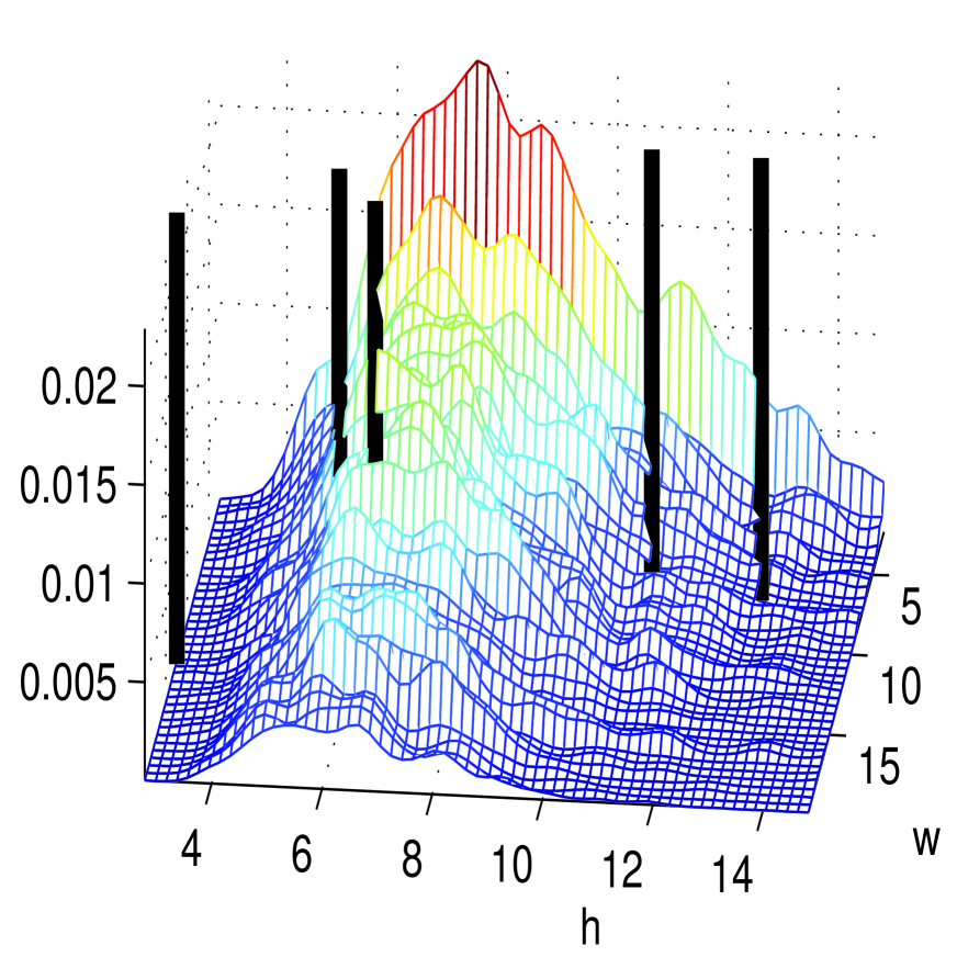
Figure 2: Bivariate distribution for the null hypothesis of angular log-frequencies $\omega$ and Lomb peak $h$ obtained from a series of 100,000 synthetic time series. The five vertical lines correspond to the five real times series. They are obtained from the lower right panel in figure 1 by locating the log-frequency and Lomb peak height of the highest peak for each data set.

The interpretation of these results is that there is a confidence level of $99.99$ % for a single peak with a log-frequency between $1$ and $2$ and a Lomb weight above $10$. This confidence interval is evaluated with respect to our initial null hypothesis of of uncorrelated (white) noise and would of course change with a different null hypothesis. Nevertheless, the confidence level achieved with the present null-hypothesis is above 99.9% and we hence expect it to remain would remain very high over a range of null-hypothesis. Also, the confidence level will also change depending on whether one assumes that the various ion concentrations are independent or not.

In conclusion, we wish to stress that the presented analysis constitute but a single case-study. Hence, it does not propose a recipe for earthquake prediction. However, we feel that the statistical evidence for this particular analysis is significant enough to encourage further studies along similar lines.

Acknowledgments: We are grateful to H. Wakita for kindly providing the data and for useful correspondence. H.S. thanks Y. Huang for collaboration at an early stage of this work and for many useful discussions. For further discussion of statistical tests and interpretations from a different point of view, see [27].

References

- [1] R.E Abercrombie and J. Mori, Nature 381, 303 (1996).
- [2] K. Maeda, Bull. Seism. Soc. Am. 86, 242 (1996).
- [3] L. Knopoff et al., J. Geophys. Res. 101, 5779 (1996).
- [4] D.D. Bowman et al., J.Geophys. Res. 103, 24359 (1998); D.J. Brehm and L.W. Braile, Bull. Seism. Soc. Am. 88, 564 (1998); S.C. Jaumé and L.R. Sykes, Pure and Applied Geophysics 155, 279 (1999).
- [5] NASDA-CON-960003, 1997, Abstracts of International Workshop on Seismo-Electromagnetics ’97.
- [6] Debate on VAN, Special issue of Geophys. Res. Lett. 23, 1291 (1996).
- [7] U, Tsunogai and H. Wakita, Science 269, 61 (1995); J. Phys. Earth 44, 381 (1996).
- [8] G. Igarashi et al., Science 269, 60 (1995).
- [9] M. Wyss, Pure Appl. Geophys. 149, 3 (1997).
- [10] R.J. Geller et al., Science 275, 1616 (1997).
- [11] A. Johansen et al., J.Phys.I France 6, 1391 (1996).
- [12] D. Sornette and C.G. Sammis, J.Phys.I France 5, 607 (1995); H. Saleur et al., J. Geophys. Res. 101, 17661(1996).
- [13] D. Sornette and Vanneste, C., Phys.Rev.Lett. 68, 612 (1992); C. Vanneste and Sornette, D., J.Phys.I France 2, 1621 (1992); D. Sornette and Andersen, J.-V., Eur. Phys. J. B 1, 353 (1998).
- [14] W.I. Newman et al., Phys. Rev. E 52, 4827 (1995).
- [15] M. Sahimi and S. Arbabi, Phys. Rev. Lett. 77, 3689 (1996).
- [16] S. Zapperi et al., Phys. Rev. Lett. 78, 1408 (1997).
- [17] S.-D. Zhang, Phys. Rev. E 59, 1589 (1999).
- [18] J.-C. Anifrani et al., J.Phys.I France 5, 631 (1995).
- [19] A. Garcimartin et al., Phys. Rev. Lett. 79, 3202 (1997).
- [20] J.V. Andersen et al., Phys. Rev. Lett. 78, 2140 (1997).
- [21] D. Sornette, J.Phys.I France 2, 2089 (1992).
- [22] D. Sornette et al., Phys. Rev. Lett. 76, 251 (1996); Y. Huang et al., Phys. Rev. E 55, 6433 (1997).
- [23] A. Johansen and Sornette, D., Int. J. Mod. Phys. C 9, 433 (1998).
- [24] D. Sornette, Phys. Reports 297, 239 (1998).
- [25] The Lomb periodogram analysis corresponds to a harmonic analysis using a series of local fits of a cosine (with a phase) with some user chosen range of frequencies. The advantage of the Lomb periodogram over a Fast Fourier transform is that the points does not have to be equidistantly sampled, which is the generic case when dealing with power laws. For unevenly sampled data, the Lomb method is superior to FFT methods because it weights data on a “per point” basis instead of “per time interval” basis. Furthermore, the significance level of any frequency component can be estimated quite accurately [26].
- [26] W.H. Press et al., Numerical Recipes (Cambridge University Press, Cambridge UK, 1992).
- [27] Y. Huang, PhD Thesis.