Effects of Non-local Stress on the Determination of Shear Banding Flow

Abstract

We analyze the steady planar shear flow of the modified Johnson-Segalman model, which has an added non-local term. We find that the new term allows for unambiguous selection of the stress at which two “phases” coexist, in contrast to the original model. For general differential constitutive models we show the singular nature of stress selection in terms of a saddle connection between fixed points in the equivalent dynamical system. The result means that stress selection is unique under most conditions for space non-local models. Finally, illustrated by simple models, we show that stress selection generally depends on the form of the non-local terms (weak universality).

Introduction—Oldroyd’s proposal [1] that any sensible rheological constitutive equation for a general fluid should obey the “admissible conditions” has had a great influence on the rheology community. In his “admissible conditions”, apart from requiring covariance, Oldroyd further imposed the “principle of frame indifference” and “locality”. de Gennes has shown that the former is no longer true if inertia effects are important [2]. Below we discuss how one must extend locality to model shear banding flow, which appears in some surfactant [3, 4, 5, 6] and polymer [7] solutions.

Shear banding has long been mooted by the polymer rheology community in connection with the spurt effect in the processing of linear polymer melts (see, e.g. Ref.[8] for a review). It is, however, in surfactant worm-like micelle solutions that the phenomena has been firmly established [3, 5, 4, 6], particularly convincingly through magnetic imaging experiments [9]. For entangled polymers or surfactant micelles, as the shear rate increases the polymers/micelles gradually align and the fluid shear thins. According to reptation theory [10, 11], the fluid shear thins so heavily that a maximum appears in the shear stress-shear rate relation at a shear rate of approximately the inverse reptation time. At high enough shear rate, the shear stress is presumed to increase again, resumably due to local (e.g. solvent) dissipation mechanisms [12]. The steady shear rate curve is qualitatively like Fig. 1. For intermediate shear rates where the slope is negative, homogeneous flow is mechanically unstable. It is found in real systems that, when the controlled shear rate increases up to the order of the inverse reptation time, the fluid becomes a composite flow profile (shear bands), where two or more bands, with alternating low and high shear rates, coexist with a common shear stress.

According to Fig. 1, there is a range of shear stress $[\sigma_{min},\sigma_{max}]$ within which the constitutive equation is multi-valued (three shear rates for a given stress), so that shear bands seem possible for any stress within $[\sigma_{min},\sigma_{max}]$. However, real systems select a well defined stress [4, 6]. We therefore need a mathematical condition, a selection criterion, which determines the coexisting stress. There are scattered results showing generically that steady state solutions behave very differently depending on whether or not the constitutive equations are local in space [16]. For local models, the final steady stress depends on the flow history [18]. Therefore an additional selection criterion must be imposed to select stress, be it variational [19, 13] or not [20, 21]. On the other hand, steady state analysis of several non-local models, either analytically [17, 22] or numerically [23, 24], yields a well-defined selected stress. It is interesting to know whether non-local effects generally lead to a stress selection criterion.

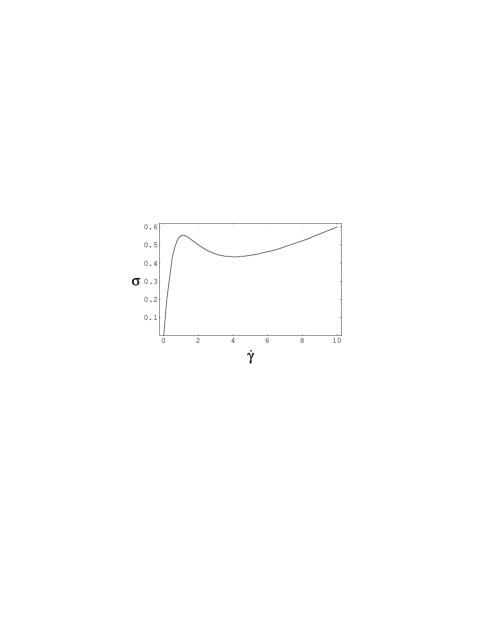
FIG. 1.: Local constitutive relation $\sigma(\dot{\gamma})$ for the Johnson-Segalman (JS) model (Eqs. 6-8) with $e=0.05$.

In this paper, we first present numerical results for the modified Johnson-Segalman (JS) model, as a concrete example of stress selection in a non-local model that has been well-studied in local form by many workers [14, 15, 13]. Although perhaps not molecularly faithful to any fluid, the JS model is a covariant model which posesses a non-monotonic flow curve, providing the necessary ingredient for a qualitative study of shear banding. We then present the main result which shows the general link between non-locality and stress selection. Finally we use simple examples to illustrate the important fact that stress selection depends on the details of the interface structure, i.e. it has weak universality.

Numerical Results for the Modified JS Model with Stress Diffusion—This model is given by

$$\rho(\partial_{t}+{\bf v}\cdot\boldsymbol{\nabla}){\bf v} = \boldsymbol{\nabla}\cdot\boldsymbol{\sigma}$$ (1)

$$\boldsymbol{\sigma} = -p\,{\bf I}+2\eta\boldsymbol{\kappa}+\boldsymbol{\Sigma}$$ (2)

$$\overset{\blacklozenge}{\boldsymbol{\Sigma}} = 2G\boldsymbol{\kappa}-\boldsymbol{\Sigma}/\tau+D\nabla^{2}\boldsymbol{\Sigma}$$ (3)

where the strain rate is $\boldsymbol{\kappa}\equiv(\boldsymbol{\nabla}{\bf v}+\boldsymbol{\nabla}{\bf v}^{T})/2$. The first equation is the momentum equation, with $\rho,{\bf v},\boldsymbol{\sigma}$ the fluid density, velocity, and stress tensor, respectively. The stress comprises the pressure $p$ (I denotes the identity matrix), the elastic stress $\boldsymbol{\Sigma}$, and a Newtonian viscous stress with viscosity $\eta$. We assume an incompressible fluid, $\boldsymbol{\nabla}\cdot{\bf v}=0$, enforced by the pressure. The non-Newtonian stress $\boldsymbol{\Sigma}$ is governed by Eq. (3), where the stress is induced by strain rate $\boldsymbol{\kappa}$ with strength described by a modulus $G$, and $\tau$ is the stress relaxation time. The Gordon-Schowalter convected time derivative is

$$\overset{\blacklozenge}{\boldsymbol{\Sigma}} \equiv \left(\partial_{t}+{\bf v}\cdot\boldsymbol{\nabla}\right)\boldsymbol{\Sigma}-\boldsymbol{\nabla}{\bf v}^{T}\cdot\boldsymbol{\Sigma}-\boldsymbol{\Sigma}\cdot\boldsymbol{\nabla}{\bf v}$$ (5)

$$+(1-a)\left(\boldsymbol{\Sigma}\cdot\boldsymbol{\kappa}+\boldsymbol{\kappa}\cdot\boldsymbol{\Sigma}\right),$$

and describes the “slip” between the polymer and fluid extension, with $a\in[-1,1]$.

Eqs. (1-3) differ from the standard JS model [25] due to the additional stress diffusion term $D\nabla^{2}\boldsymbol{\Sigma}$ in Eq. (3). El-Kareh and Leal [26] have analyzed the microscopic dumbbell model (i.e. the case $a=1$) and derived this term, representing the diffusion of the stress carrying element. Note the important difference that the standard JS model is a local model, whereas Eq. (3) is not.

Given a shear stress value $\sigma_{xy}$, we look for the steady planar shear flow numerically. For ${\bf v}=v(y,t)\hat{{\bf e}}_{x}$, the modified JS model reduces to [13]

$$\sigma = S+e\dot{\gamma}$$ (6)

$$\tau\partial_{t}S = \hat{D}\partial^{2}_{y}S-S-\dot{\gamma}N+\dot{\gamma}$$ (7)

$$\tau\partial_{t}N = \hat{D}\partial^{2}_{y}N-N+\dot{\gamma}S$$ (8)

The rescaled variables are defined as $\sigma=\sqrt{1-a^{2}}\ \sigma_{xy}/G$, $S=\sqrt{1-a^{2}}\ \Sigma_{xy}/G$, $N=[(1-a)\Sigma_{xx}-(1+a)\Sigma_{yy}]/2G$, $\hat{D}=\tau D$, $\dot{\gamma}=2\sqrt{1-a^{2}}\ \tau\kappa_{xy}$, and $e=\eta/G\tau$. Because the steady planar shear flow solution of Eq. (1) has zero Reynolds number (and most macromolecular dynamics are in this limit) we can use the low Reynolds number limit ($\rho\rightarrow 0$), Eq. (6), to obtain the same steady solution. Eqs. (7-8) are the non-trivial dynamics of $\boldsymbol{\Sigma}$ (other components are uncoupled). Note that there is only one non-dimensional parameter $e$ (the viscosity ratio) in the steady state problem.

Given $\sigma$, we integrate Eqs. (6-8) over time $t$ to see whether a steady state banding solution can be reached. During the integration, the values of $S$ and $N$ at the two ends $y=\pm y_{0}$ are fixed to those of the high and low strain rate branches respectively. At $t=0$, the functions $S(y)$ and $N(y)$ are chosen arbitrarily as $C_{1}\tanh y+C_{2}$, with the constants $C_{1}$, $C_{2}$ fixed by the boundary conditions. The value $y_{0}$ is chosen to be sufficiently large that its exact value is irrelevant. We find that a steady (elementary) shear band solution can be found only at a specific shear stress value, $\sigma=\sigma_{0}$. If the stress value is too large or too small, one of the phases shrinks completely. The values $\sigma_{0}$ as a function of the model parameter $e$ are shown in Fig. 2. Note that in an infinite system $\sigma_{0}$ does not depend on the diffusivity $D$, which just sets the interface width. However, anisotropic diffusion (a fourth rank tensor $\boldsymbol{D}$ in Eq. 3), may lead to diffusivity dependent selection.

FIG. 2.: The selected stress $\sigma_{0}$ of the modified Johnson-Segalman model as a function of the viscosity ratio $e$. The limits $\sigma_{min}(e)$ and $\sigma_{max}(e)$ are also shown.

Nontransverse Saddle Connection—We have shown above that a non-local model can select the stress sharply. Now we show that, in general, a non-local model in planar shear flow selects stress sharply (could be uniquely), provided that the model is a differential equation and satisfies rotational and Galilean invariance.

1. To begin, we observe that the steady state equations, like Eqs. (6-8) without time derivatives, comprise a set of ordinary differential equations (ODE) for the independent dynamical variables $\{\psi_{i}\}$ ($S$ and $N$ for the JS model), rather than partial differential equations (PDE), since only differentiation in the velocity gradient direction, say ${\bf\hat{y}}$, is present in planar shear flow. The phase space for the equivalent first order ODE is $\left[\left\{\psi_{i}\right\},\left\{\partial_{y}\psi_{i}\right\},\left\{\partial^{2}_{y}\psi_{i}\right\},\ldots\right]$. Higher order gradients in the original PDE would entail a ODE phase space with large dimension.

2. To each homogeneous steady flow (a phase) there corresponds a fixed point ($\left[\left\{\psi^{\ast}_{i}\right\},0,0,\ldots\right]$) in the ODE phase space since, by definition, homogeneous flow means the variables do not change with $y$ [27].

3. If the interface width is small compared to the other length scales in the problem, e. g. the distance between two neighbouring interfaces, it is sufficient to consider an elementary shear banding solution, which describes, in a planar geometry, a composite flow with a smooth interface separating a single region of material in the high shear rate phase from a single region of material in the low shear rate phase. Mathematically, the elementary shear band is a solution of the ODE which asymptotically connects the high and low shear rate phase fixed points between $y=\pm\infty$. Since the fixed points are both saddle points (see below) and distinct, the elementary shear band solution is a heteroclinic saddle connection [28].

4. Let the attractor and repellor basins [28] of one fixed point, say $A$, have dimensions $a(A)$ and $r(A)$ respectively. Another fixed point $B$ has similarly defined $a(B)$ and $r(B)$. Note that if the phase space has dimension $d$ (for the modified JS model $d=4$), then $a(A)+r(A)\leq d$ and $a(B)+r(B)\leq d$. A saddle connection joins two fixed points, so that it is an intersection of the repellor of one fixed point, say $A$, and the attractor of the other fixed point $B$. We denote its dimension $s(A,B)$ [30]. In the ODE phase space, the intersection is at least one dimension, so that $s(A,B)\geq 1$. There is a trivial inequality $r(A)+a(B)-s(A,B)\leq d$. If equality holds the saddle connection is called transverse: it is formed by a robust intersection of two manifolds, and is structurally stable against small perturbations of the ODE parameters (in the modified JS model, $\sigma$ and $e$). The case $r(A)+a(B)-s(A,B)<d$ is called non-transverse, and the corresponding saddle connection is structurally unstable. It is important to recognise that if the elementary shear band solution is a non-transverse saddle connection, a small change of the shear stress (a parameter in the ODE) will remove the saddle connection, which gives a very sharp stress selection. In another words, given an existing shear band solution, a stress perturbation is singular if it is of the non-transverse type saddle connection. On the other hand, if there is a transverse saddle connection shear band solution, one can perturb the stress to obtain a (slightly) different shear band solution. Therefore, there is no stress selection for a transverse saddle connection. (Stress perturbation becomes a regular perturbation.)

5. We now prove that: if the model has rotational and Galilean invariance, a shear band solution in planar shear flow must be non-transverse. Let us momentarily assume that there is a transverse saddle connection approaching, say, fixed point $A$ at $y=-L$ to fixed point $B$ at $y=L$. Galilean invariance allows us to choose an inertial frame in which the flow velocity $v_{x}(y=\pm L)=\pm V$. Since the bulk are rotationally invariant and the boundary conditions are symmetric under rotation by 180 degrees, one can rotate the solution around the vorticity ($z$) axis by 180 degrees to obtain a different shear band solution which obeys the same equation and the same boundary condition (e.g. ${v_{x}(\pm L)=\pm V}$). This solution approaches fixed point $B$ at $y=-L$ to fixed point $A$ at $y=L$. Fixed points $A$ and $B$ have both attractor and repellor directions, and are thus saddle points. Now take the (thermodynamic) limit $L\rightarrow\infty$ so that the above two solutions become saddle connections. The two saddle connections are related by the symmetry transformations, so are of the same type (both transverse). A contradiction now appears, since “there are not enough dimensions to put two transverse saddle connections in the phase space”. Formally, the transverse condition leads to $r(A)+a(B)=d+s(A,B)>d$ and $r(B)+a(A)=d+s(B,A)>d$, therefore $a(A)+r(A)+a(B)+r(B)>2d$. However, from $a(A)+r(A)\leq d$ and $a(B)+r(B)\leq d$ we have $a(A)+r(A)+a(B)+r(B)\leq 2d$. So the shear band cannot be a transverse saddle connection.

Weak Universality—One important aspect of stress selection can be illustrated by a simple model inspired by the macromolecular character of many systems exhibiting non-linear rheology. Let the shear stress $\sigma$ be

$$\sigma=F(\dot{\gamma})+\eta\,\dot{\gamma}_{loc},$$ (9)

where the first, non-linear, part associated with macromolecules is sensitive to a locally averaged shear rate $\dot{\gamma}$ as opposed to the second, Newtonian, part attributed to solvent, which is sensitive to the true local shear rate $\dot{\gamma}_{loc}$. We approximate the local averaging from $\dot{\gamma}_{loc}$ to $\dot{\gamma}$ by a gradient expansion, $\dot{\gamma}=\left(1-R^{2}(\dot{\gamma})\nabla^{2}+\ldots\right)^{-1}\dot{\gamma}_{loc}$, and hence

$$\dot{\gamma}_{loc}\simeq\left(1-R^{2}\left(\dot{\gamma}\right)\nabla_{y}^{2}\right)\dot{\gamma}$$ (10)

We anticipate sensitivity of the non-local scale $R(\dot{\gamma})$ to $\dot{\gamma}$ through distortion of the macromolecular shape.

In terms of the locally averaged shear rate $\dot{\gamma}$ we have

$$\sigma=f(\dot{\gamma})-\eta R^{2}(\dot{\gamma})\nabla_{y}^{2}\dot{\gamma}$$ (11)

where $f(\dot{\gamma})\equiv F(\dot{\gamma})+\eta\,\dot{\gamma}$ is, as before, the steady (and constant) shear rate flow curve as exemplified in Fig.1. Multiplying Eq. (11) by $R^{-2}(\dot{\gamma})\nabla_{y}\dot{\gamma}$ and integrating $y$ across the shear band leads to

$${\cal D}(\sigma)\equiv\int^{\dot{\gamma}(\infty)}_{\dot{\gamma}(-\infty)}\frac{f(\dot{\gamma})-\sigma}{R^{2}(\dot{\gamma})}d\dot{\gamma}=\left[\frac{\eta}{2}(\nabla_{y}\dot{\gamma}(y))^{2}\right]_{y=-\infty}^{y=\infty}$$ (12)

where $\dot{\gamma}(y=\pm\infty)$ depends on $\sigma$ through $f(\dot{\gamma}(y=\pm\infty))=\sigma$. Since $\nabla_{y}\dot{\gamma}(y=\pm\infty)=0$, an interfacial profile must satisfy ${\cal D}(\sigma)=0$, which is the condition to select the stress.

According to Eq. (12), different functions $R(\dot{\gamma})$ give different ${\cal D}(\sigma)$, and hence different selection criteria ${\cal D}=0$! Therefore, two models with different $R(\dot{\gamma})$ but the same behaviour in homogeneous flow, $f(\dot{\gamma})$, can behave differently upon forming shear bands. The simple case $R(\dot{\gamma})$ independent of $\dot{\gamma}$ corresponds to the equal areas construction speculated upon by Ref. [13], and cannot be regarded as generic. Stress selection has weak universality, implying that impurities or other effects which changes the interfacial properties could in principle affect quantities like $R(\dot{\gamma})$ and hence alter the selected shear stress.

For equilibrium transitions, with coexistence equations analogous to Eq. (11), terms involving gradients would be exactly integrable without an integrating factor ($1/R^{2}(\dot{\gamma})$ in Eq. 12) because they arise from a functional derivative of a coarse-grained free energy. The resulting interface solvability condition (i.e. a Maxwell construction) is independent of the detailed gradient terms, in contrast to the weak universality discussed above. Discussion—We close with a few comments. First, we have not proven existence of shear banding solutions. There are physical phenomena where coexistence between bulk states is prohibited because it is unfavourable to form an interface, and robust hysteresis can be expected. Gel swelling provides a beautiful example.

Secondly, the non-transversality condition of the saddle connection is, strictly speaking, weaker than uniqueness. There are two possible situations where uniqueness may fail. The first situation happens when, due to an accidental situation, the attractive basin of one fixed point and the repelling basin of the other fixed point move so as to maintain the saddle connection upon changing the shear stress $\sigma$ as a control parameter. The second situation happens when more than one isolated stresses are selected, i.e. uniqueness fails globally. These have negligible chance to be realised in a model. Should it happen, one may ask for a physical argument for the degeneracy to be sure that it is not a mathematical artfact. Generally, uniqueness of the stress selection can be expected for models with gradient terms

An interesting question is whether the stress selected by non-local effects can be obtained by a variational principle. A conventional variational principle, like the one used for the equilibrium phase transitions, relies on the volume contribution to a universal functional and gives a criterion insensitive to the interfacial structure [29], because the interface only contributes a vanishing fraction if the total volume is assumed to be large. The model Eq. (11), illustrates that the way non-local effects select stress is different from a variational principle based on such a universal functional. Therefore the obvious choices of either free energy or entropy production cannot generally represent the selection criterion posed by the non-local effects.

After this manuscript was submitted, Yuan published a similar modification to the JS model [31].

Acknowledgments—We thank A. Ajdari, M. Cates, B. L. Hao, and O. Radulescu for fruitful conversations.

REFERENCES

- [1] J. G. Oldroyd, J. Non-Newt. Fluid Mech. 14, 9 (1984).
- [2] P.-G. de Gennes, Physica 118A, 44 (1983). G. Ryskin, Phys. Rev. A 32, 1239 (1985).
- [3] H. Rehage and H. Hoffman, Mol. Phys. 74, 933 (1991).
- [4] J.-F. Berret, D. C. Roux, and G. Porte, J. Phys. (France) 4, 1261 (1994).
- [5] V. Schmitt, F. Lequeux, A. Pousse, and D. Roux, Langmuir 10, 955 (1994).
- [6] C. Grand, J. Arrault, and M. E. Cates, J. Phys. II (France) 7, 1071 (1997).
- [7] P. T. Callaghan, private communication.
- [8] M. M. Denn, Ann. Rev. Fluid Mech., 22, 13 (1990).
- [9] P. T. Callaghan, M. E. Cates, C. J. Rofe, and J. B. A. F. Smeulders, J. Phys. II (France) 6, 375 (1996).
- [10] M. Doi and S. F. Edwards, The Theory of Polymer Dynamics (Clarendon, Oxford, 1989).
- [11] M. E. Cates, J. Phys. Chem. 94, 371 (1990).
- [12] N. A. Spenley and M. E. Cates, Macromolecules 27, 3850 (1994).
- [13] F. Greco and R. C. Ball, J. Non-Newt. Fluid Mech. 69, 195 (1997).
- [14] D. S. Malkus, J. S. Nohel, and B. J. Plohr, J. Comp. Phys. 87 (1990) 464; SIAM J. Appl. Math. 51 (1991) 899.
- [15] Y. Y. Renardy, Th. Comp. Fl. Mech. 7, 463 (1995).
- [16] From our point of view, 2D flow solver results which show a selected stress for a local model [17] should be examined further to see whether the algorithm implicitly introduced non-locality (numerical diffusion).
- [17] N. A. Spenley, X. F. Yuan, and M. E. Cates, J. Phys. II (France) 6, 551 (1996).
- [18] P. D Olmsted, O. Radulescu, and C.-Y. D. Lu, in preparation (1999).
- [19] G. Porte, J. F. Berret and J. L. Harden, J. Phys. II (France) 7, 459 (1997).
- [20] M. E. Cates, T. McLeish, G. Marrucci, Europhys. Lett. 21, 451, (1993).
- [21] V. Schmitt, C. M. Marques, and F. Lequeux, Phys. Rev. E52, 4009 (1995).
- [22] J. R. A. Pearson, J. Rheol. 38, 309 (1994).
- [23] P. D. Olmsted and P. M. Goldbart, Phys. Rev. A41, 4578 (1990); ibid, A46, 4966 (1992).
- [24] P. D. Olmsted and C.-Y. D. Lu, Phys. Rev. E 56, R55 (1997).
- [25] R. G. Larson, Constitutive Equations for Polymer Melts and Solutions, (Butterworth, Boston,1988).
- [26] A. W. El-Kareh and L. G. Leal, J. Non-Newt. Fl. Mech. 33, 257 (1989).
- [27] Note that although the velocity is not a constant, it cannot enter the equation of motion alone, due to Galilean invariance.
- [28] R. H. Abraham and C. D. Shaw, Dynamics – The Geometry of Behavior, 2nd. ed., (Addison-Wesley, NY, 1992).
- [29] It is possible to have a functional whose bulk contribution is indifferent to the interface location, in which case the interface contribution plays the decisive role.
- [30] We assume and are the only singular points on the saddle connection, so that does not change along the connection.
- [31] X.-F. Yuan, Europhys. Lett. 46, 542, (1999).