Transport properties and phase diagram of the disordered lattice vibration model

Abstract

We study the transport and localization properties of scalar vibrations on a lattice with random bond strength by means of the transfer matrix method. This model has been recently suggested as a means to investigate the vibrations and heat conduction properties of structural glasses. In three dimensions we find a very rich phase diagram. The delocalization transition is split, so that between the localized and diffusive phases which have been identified in the Anderson problem, we observe a phase with anomalous, sub-exponential localization. For low frequencies, we find a strongly conducting phase with ballistic and super-diffusive transport, reflecting a diverging diffusivity. The last phase generates an anomalous heat conductivity which grows with the system size. These phases are the counterparts of those identified in an earlier study of the normal modes.

1 Introduction

It is well known that disorder in the parameters of physical models can induce scattering and localization, and the most outstanding example is the electronic Anderson model. This model has been the focus of a large set of theoretical, numerical and experimental studies over the last three decades, and there is an enormous literature on various aspects of this problem. At the same time, the related problem of vibrations in disordered materials received almost no attention, although structural disorder is very common in glasses and other disordered materials.

It is well known that in low temperatures there are several features common to most glasses. An outstanding phenomenon is the existence of an anomalous heat conductivity at low temperature, a plateau in the heat conductivity in a higher temperature range, and no decrease in it at higher temperatures [1]. It is not clear if those effects are the results of nonlinear phenomena [2] or of harmonic vibrations [3, 4]. A calculation of transport in a vibration model is a good way of testing whether the main mechanism of heat conductance in glasses is obtained from the linear harmonic vibration modes, or if nonlinear scattering processes have to be invoked.

Since vibration Hamiltonians are elastically stable there are special constraints on the dynamics. Therefore, though the dynamical equations are similar to the Anderson problem of a quantum particle in a random potential there are some major diffrences due to these constraints. This model is a random Laplacian model, with positive off diagonal coefficients. It leads to the existence of a global translation mode at zero frequency. This features has a decisive influence on the entire spectrum of vibrations at low frequencies. Other distinguishing features are the vector character of the vibrations, and in the case of a two (or more) component systems, random masses. We will comment in more detail on these differences in section 2.

The focus of this study is a scalar lattice vibration model with random elastic coefficients, and equal masses. This model disregards some of the important features of glass vibrations. Nevertheless, in a previous work which focused on the eigenstates [5], it was shown that this model contains many of the interesting features of glass vibrations, and is qualitatively different from the usual electronic models. The present work reveals the phase diagram and the conductance properties of the disordered lattice model. We note that the model under discussion also describes a free quantum particle with disorder in its transport behavior.

In our study we find several new qualitative features that are absent in the classical Anderson problem. Some theoretical studies were vibration problems with disorder, such as [6, 8], have concluded that they belong to the same universality class as the Anderson model. This is not the case for in the model studied here and in [5].

We outline the main differences: In the three dimensional electronic Anderson model there are two phases: diffusive with extended states and localized. In the vibrational case there are four phases. In addition to the two phases familiar from the Anderson problem there is an insulating sub-exponentially localized phase with multifractal normal modes, and a strongly conducting phase, with states characterized by weak scattering, and a well defined wavelength. The phase diagram is displayed in fig. 1, and described in detail in section 3.

Figure 1: Phase diagram of the vibration model in three dimensions: Regions of different qualitative transport behavior, as a function of the frequency $\omega$, for a fixed disorder distribution. The small $\omega$ region below the dashed line is present only in finite systems. The descriptions given in italics refer to normal modes, analyzed in [5]. The symbols appearing in the diagram are the finite size localization length $\xi_{W}$ for a system of width $W$, the conductance $G_{W}$ of a finite cubic system of side $W$, and the conductivity $g$. They are explained in detail in section 3.

In two dimensions the Anderson model is insulating with exponential localization and all the states are multifractal, while in the vibrational case exponential localization is also observed, but a transition occurs between multifractal and extended modes, accompanied by a singularity in the localization length. This is discussed in detail in our paper on the two dimensional case [7].

The former study [5] concentrated on a numerical study of the properties of the normal modes. In the present paper we apply the transfer matrix method [9] to the vibration model. This method has the advantage of pointing out precisely the transition between conducting and insulating behavior through localization. The finite size scaling analysis which has been used earlier to calculate the physical quantities now reveals the presence of additional length scales. The method also provides a direct tool for calculating the conductance of finite systems. The various numerical methods which are used to analyze the Anderson model, and the results obtained have been recently reviewed by [10].

The structure of the paper is as follows: in section 2 we define the model, the numerical method, and explain how the numerical data are used to study the system. Section 3 describes in detail the results in the three dimensional case, emphasizing the different qualitative behaviors. In section 4 we apply the results of section 3 to calculate the thermal conductivity as a function of temperature. The paper is concluded with a discussion of the relevance of our results to glasses.

2 The disordered harmonic model and elastic energy transport

The vibration problem in glasses is a vector problem which is defined for a disordered lattice where both structural and elastic disorder play a major part. In this paper we treat a simpler variant of this problem: the scalar vibration model. The model under consideration is defined on a $d$-dimensional simple cubic lattice with periodic boundary conditions. It consists of a scalar field which is subject to elastic equations of motion. For a normal mode of frequency $\omega$ the field equations read

$$-\omega^{2}\phi(\vec{x})=\sum_{y,\,|\vec{y}-\vec{x}|=1}k_{\vec{x},\vec{y}}[\phi(\vec{y})-\phi(\vec{x})]\ ,$$ (1)

where $\vec{x}$ and $\vec{y}$ denote lattice sites. The $k$’s are symmetric ($k_{\vec{x},\vec{y}}=k_{\vec{y},\vec{x}}$), positive, independent and identically distributed random numbers. A similar model was introduced recently by [11] to describe boson peaks in glasses.

This model is in fact a realization of the Anderson tight binding model with special constraints. The diagonal terms are the sum of the off diagonal terms in the same row, and the off diagonal terms are real and positive number. The same model describes free particle.

The focus of the present study is the transport properties of this model. For this purpose it is convenient to single out a preferred direction, and label the coordinate in this direction by $t$. We define a column vector $v_{t}$ whose components are the values of $\phi$ at the sites on the hyperplane labeled by $t$. It is then possible to use eq. (1) to express $v_{t+1}$ in terms of $v_{t}$ and $v_{t-1}$. This linear relation defines a random transfer matrix $T$ by

$$\pmatrix{v_{t+1}\cr v_{t}}=T_{t}\pmatrix{v_{t}\cr v_{t-1}}\ .$$ (2)

The transfer matrices $T$ have the same non-zero elements as those of the Anderson tight-binding model.

Following the standard methods developed in the context of disordered electronic systems, we study the conductance properties using the Lyapunov spectrum of the product

$$\cdots T_{t}T_{t-1}\cdots T_{1}\ .$$ (3)

Due to the left-right symmetry of the problem, the Lyapunov exponents come in pairs of opposite signs. For any positive value of $\omega^{2}$, and for non-vanishing disorder all the exponents are non-zero, signaling that in a quasi-1D geometry the system is always insulating. The smallest of the non-zero exponents may be identified with the best conducting channel, so that it gives the inverse of the finite size localization length $\xi_{W}$, where $W$ is the transverse size of the system.

We study $\xi_{W}$ as a function of $W$, with the aim of finding the asymptotic behavior for large $W$. The following types of asymptotics are known to occur in models of electronic localization

1. The localization length saturates to a finite value $\xi_{W}\rightarrow\xi_{\infty}=const\ .$ This is the localized phase which is expected to characterize systems with strong disorder, and low dimensionality.

2. The critical state, $\xi_{W}\sim W$. This behavior is commonly associated with the delocalization transition, using the scaling hypothesis.

3. The diffusive phase, $\xi_{W}\sim DW^{d-1}$. This phase is expected to have Ohmic behavior,

   $$G\sim gW^{d-2}\ ,$$ (4)

   and the conductivity $g$ is proportional to $D$,

Since the transverse size of the system which can be studied numerically is limited, the extrapolation to infinite size can be improved significantly using finite-size scaling (FSS) [9], which assumes a scaling form

$$\xi_{W}=\xi_{\infty}f(W/\xi_{\infty})\ ,$$ (5)

with different scaling functions above and below the transition. The localization length $\xi_{\infty}$ is found numerically to diverge as

$$\xi_{\infty}\sim|\sigma-\sigma_{c}|^{-\nu}\ ,$$ (6)

in three dimensions and as

$$\xi_{\infty}\sim\exp\left(\sigma^{-\nu^{\prime}}\right)\ ,$$ (7)

in two dimensions where $\sigma$ measures the disorder strength, and $\sigma_{c}$ is the critical value of disorder in three dimensions.

The average conductance $G$ is given, using the the entire set of Lyapunov exponents $\gamma_{j}$, by

$$G=\sum{1\over\cosh^{2}(\gamma_{j}W)}\ ,$$ (8)

for a hypercubic sample [13]. We will show below that in the diffusive state, since the spacing between the Lyapunov exponents is slowly varying, the conductivity $g$ is indeed proportional to $D$. However, this is not always valid, and we show below that the relation between $g$ and $D$ breaks down when scattering is too weak.

Here, we study the transport properties for different values of $\omega$, rather than disorder. As expected, we find that small $\omega$ corresponds in many ways to weak disorder; the basic reason for this is that the uncorrelated disorder is averaged out in its effect on large wavelength modes, which correspond to small $\omega$. However, the mapping between small $\omega$, and weak noise is exact only in one dimension [12]. We find that the behavior as a function of $\omega$ is considerably more involved than that which is known for electronic models, and which has been reviewed above. We find several new phases, and conclude that in three dimensions the simple scaling picture of the localization transition does hold for our model. As a result, FSS does not hold in the simple form (5), and has to be modified. The present study confirms and adds further information to the new features which were discovered in the geometry of the eigenmodes of the same model [5].

3 Transport properties in three dimensions

As described is section 2, the various phases of the system can be characterized by the asymptotic behavior for large transverse width $W$ of the the finite size localization length $\xi_{W}$ which is the inverse of the smallest non-negative Lyapunov exponent and of the conductance $G$ which is defined in terms of the Lyapunov exponents in (8). The results of this section were obtained for the model (1) in a bar shaped geometry, with a square cross section of width $W$, and a fixed distribution of the values of the elastic constants $k_{\vec{x},\vec{y}}$: A binary distribution with ${\sf Prob}(k=0.1)=0.8$ and ${\sf Prob}(k=1)=0.2$. We computed the Lyapunov exponents of the product (3) for different values of $W$, $5\leq W\leq 16$. The number of realizations which were multiplied was between $4\times 10^{6}$ for the smallest widths, and $2.5\times 10^{5}$ for the largest.

We studied the transport properties for varying $\omega$. These results are summarized in the phase diagram displayed in fig. 1. We sketch the major features of the phase diagram. For frequencies which are higher then $\omega_{1}$ we observe a normal localized phase with exponential localization. However in the transition range near $\omega_{1}$, the usual finite size scaling ansatz fails, and a modified finite size scaling with two parameters is needed to rescale the data. For smaller frequencies in the range $\omega_{2}<\omega<\omega_{1}$ we observe a divergence of the finite localization length as a non-trivial power of the system size in the entire range available to us. This phase is interpreted as being sub-exponentially localized. In the range $\omega_{3}<\omega<\omega_{2}$ we observe the normal diffusive behavior familiar from electronic models, but finite size scaling has again to be modified near the transition. These effects are related to a continuous change in the multifractal exponents of the normal modes in this range, instead of a sharp transition.

At frequencies which are lower than $\omega_{3}$, the normal diffusive behavior is replaced by an irregular dependence of the transport properties on the system parameters. The diffusion coefficient becomes hard to define numerically, and a variety of types of size dependence of the conductance is observed. Since $\omega<\omega_{3}$ is the range corresponding to weak scattering as found in [5], these effects can be interpreted as residuals of the ballistic propagation between scattering events. We expect a long crossover region before an ultimately diffusive behavior can be observed.

The rest of this section is devoted to a detailed description of the phases in the order they appear with decreasing $\omega$.

3.1 The normal localized phase

The system is localized for values of $\omega^{2}\geq\omega_{1}^{2}=1.1$. This phase is characterized by the existence of a finite limiting localization length

$$\xi_{\infty}=\lim_{W\rightarrow\infty}\xi_{W}<\infty\ ,$$ (9)

which we conventionally identify with the range of the Green’s function of eq. (1)

$$\xi_{\infty}=\lim_{|\vec{x}-\vec{y}|\rightarrow\infty}-{1\over|\vec{x}-\vec{y}|}\left<\log|{\cal G}(\vec{x},\vec{y};\,\omega)|\right>\ .$$ (10)

We found that in the localized phase the dependence of $1/\xi_{W}$ on $1/W$ is well approximated as linear. This function can then be linearly extrapolated to $1/W=0$, giving an estimate for $1/\xi_{\infty}$. The values of $\xi_{\infty}$ thus obtained are listed in table 1 for various values of $\omega^{2}$.

$\omega^{2}$	$\xi_{\infty}$	$\log_{10}a$	$\log_{10}b$
2.0	0.377
1.6	0.131
1.4	0.226	-0.16
1.3	0.259	-0.21
1.25	0.160	-0.02
1.2	0.094	0.22
1.17	0.073	0.33
1.15	0.047	0.56
1.14	0.033	0.73
1.135	0.026	0.85
1.13	0.019	0.97	-0.003
1.125	0.013	1.11	-0.007
1.12	0.008	1.20	-0.015
1.115		1.30	-0.022
1.112		1.37	-0.026
1.11		1.37	-0.028
1.105		1.44	-0.031

Table 1: The values of the localization length $\xi_{\infty}$ as determined by extrapolation to $W=\infty$, and the parameters $a$ and $b$ of the modified FSS (5), as a function of $\omega^{2}$ in the localized phase in three dimensions. The values missing from the table could not be determined significantly numerically, except when a value is given for $a$ and not for $b$, where $b$ was fit to 1. The different symbols were obtained for different values of $\omega$, all of which are given in table 1.

As can be seen from table 1, the value $\xi_{\infty}$ increases as $\omega^{2}$ decreases as it starts to diverge near the transition. However, because of the limited size of the systems which were measured, near the transition the precision of the measured $\xi_{\infty}$ deteriorates, until all precision is lost. As discussed in section 2 above, this difficulty is commonly dealt with by invoking the FSS hypothesis (5), which can be written equivalently as $\log(\xi_{W}/W)=g(\log W-\log\xi_{\infty})$; $\xi_{\infty}(\omega)$ is then determined so that the various curves of measured $\log(\xi_{W}/W)$ versus $\log W$ collapse.

This procedure works well for $\omega^{2}\geq 1.14$. However, for $\omega_{1}^{2}=1.1\leq\omega^{2}\leq 1.14$ the numerical curves do not collapse implying that FSS is violated. It is nevertheless possible to describe the measured values of $\xi_{W}$ for all $\omega^{2}$ using a modified form of FSS

$${\xi_{W}\over W}=b(\omega^{2})f\left({W\over a(\omega^{2})}\right)\ ;$$ (11)

the values of $\log a$ and $\log b$ thus obtained are also reported in table 1, and the resulting data collapse is displayed in fig. 2. Unfortunately the fitting parameters $a$ and $b$ are not directly related to the localization length, and therefore the modified FSS is not useful for a measurement of $\xi_{\infty}$ near the transition. The physical interpretation of $a$ and $b$ remains unclear. For $\omega^{2}\geq 1.14$, where $b=1$, $a$ may be again identified with $\xi_{\infty}$, which gives values in accord with those obtained from direct extrapolation.

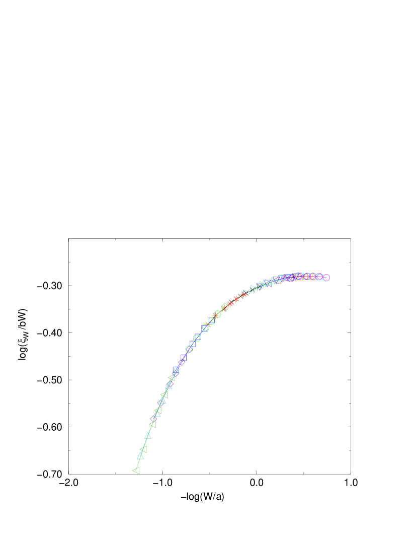
Figure 2: Modified finite size scaling in the localized phase in three dimensions. $W$ is the width, and $\xi_{W}$ is the finite size localization length; the logarithms are in base 10. The data displayed are for $1.105\leq\omega^{2}\leq 1.4$. The FSS parameters $a$ and $b$ as functions of $\omega$ are reported in table 1

As discussed above, $\xi_{\infty}$ diverges at the transition, but it is difficult to measure this divergence accurately. Nevertheless, the values of $\xi_{\infty}$ obtained by direct extrapolation are well in accord with a power like divergence

$$\xi\sim(\omega-\omega_{1})^{-\nu_{1}}$$ (12)

with $\nu_{1}\sim 1.7$. This value is within the numerical errors in agreement with the value of $\nu=1.5$ reported for the three-dimensional Anderson transition [13]. On the other hand, the fitting parameters $a$ and $b$ increase very slowly near $\omega_{1}$, and their rate of divergence was impossible to determine to a reasonable accuracy, from the numerical measurement. The breakdown of FSS implies there is at least one more length scale, $\xi_{*}$, in the system in addition to $\xi_{\infty}$(and $W$); unlike $\xi_{\infty}$, $\xi_{*}$ does not diverge at the transition.

3.2 The anomalous localized phase

This subsection describes the properties of the system for $\omega_{2}^{2}=0.96\leq\omega^{2}\leq\omega_{1}^{2}=1.1$. In electronic models the Anderson transition in three dimensions is the boundary between localized and conducting diffusive phases. In the present model the qualitative behavior is markedly different. One surprising feature is that the finite size localization length $\xi_{W}$ for a given $W$ viewed as a function of $\omega^{2}$ has a maximum at the the transition point $\omega^{2}=1.1$. That is, the conductivity of a finite sample becomes worse when $\omega$ is decreased from the transition, the opposite of what would occur if the transition were into a conducting phase. This trend continues until a minimum is reached at $\omega^{2}=1.0$, and the usual situation whereby $\xi_{W}$ increases with decreasing $\omega^{2}$ is restored (see fig. 3).

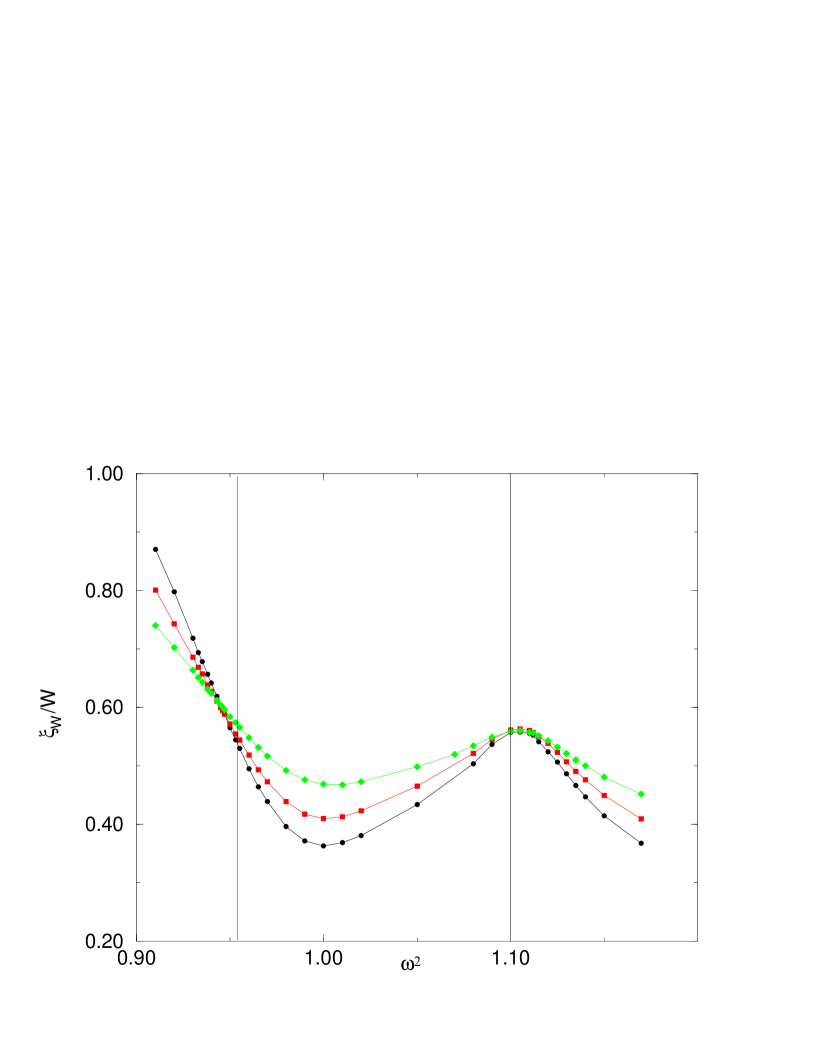
Figure 3: Finite size localization length $\xi_{W}$ divided by the width $W$, as a function of the frequency squared $\omega^{2}$, for widths $W=5,\,8,\,12$, from top to bottom. The vertical lines show the limits of the anomalous localized phase.

The behavior for a fixed $\omega$ as a function of $W$ is also unusual. $\xi_{W}$ does not saturate to a finite value, and continues to grow with $W$ as some non-trivial power

$$\xi_{W}\sim W^{\beta}\ ,\qquad 0<\beta<1\ .$$ (13)

Some examples are given in fig. 4, where a clear power law behavior is observed, in contrast with the other phases.

Figure 4: The base 10 logarithm of the Finite size localization length $\xi_{W}$ divided by the width $W$, versus $\log_{10}W$, shown for three frequencies in the anomalous localized range. The full, dashed, and dot-dashed lines refer to $\omega^{2}=1.08,\,1.00,\,0.97$ respectively.

The measured values of $\beta$ are reported in table 2, and the minimum occurs at $\omega^{2}=1$. An interesting feature is that the at the lower bound of this phase $\beta$ is still significantly smaller than 1; we discuss below the implication of this fact on the nature of the second phase transition into the diffusive phase.

$\omega^{2}$	$\beta$	$\xi_{*}$
1.10	1.00
1.09	0.97	0.93
1.08	0.93	0.95
1.05	0.84	0.87
1.02	0.74	0.98
1.01	0.73	0.95
1.00	0.71	1.00
0.99	0.72	1.03
0.98	0.75	1.08
0.97	0.81	1.15
0.965	0.85	1.25
0.96	0.88	1.40

Table 2: The localization exponent $\beta$ and the anomalous localization length $\xi_{*}$ as a function of $\omega^{2}$, in the anomalous localized phase.

The asymptotics of $\xi_{W}$ given in eq. (13) shows that the Green’s function in this phase is certainly not localized with a finite localization length $\xi_{\infty}$ in the sense defined in (10). However, it is compatible with a weaker ‘stretched exponential’ localization

$$\left<|{\cal G}({\vec{x}},{\vec{y}})|\right>\sim\exp\left[-\left({|{\vec{x}}-{\vec{y}}|\over\xi_{*}}\right)^{\alpha}\right]\ ,$$ (14)

with $0<\alpha<1$. If the three dimensional system indeed behaves as in (14) then we can expect the same behavior in the bar geometry which we studied for distances $|{\vec{x}}-{\vec{y}}|$ which are small compared to $\xi_{W}$, which marks the crossover to true exponential decay. If $W\gg\xi_{*}$, we can estimate $\xi_{W}$ by demanding that the two types of decay are of the same order of magnitude for distances of order $W$, that is,

$$\exp\left[-\left({W\over\xi_{*}}\right)^{\alpha}\right]\sim\exp\left[-{W\over\xi_{W}}\right]\ .$$ (15)

This yields the estimate

$$\xi_{W}\sim W^{1-\alpha}\xi_{*}^{\alpha}\ ,$$ (16)

which agrees with (14) identifying $\beta=1-\alpha$.

The delocalization at $\omega\to\omega_{1}$ from below, as described in this section, occurs because $\beta\to 1$, and the length $\xi_{*}$ remains finite. It seems natural therefore to identify $\xi_{*}$ with the additional length scale present in the normal localized phase.

The transition in $\omega_{2}$ is unique since $\alpha(\omega_{2})>0$. One has a stretched exponential correlation with an internal length $\xi*$ which should diverge to infinity at the transition. This is analog to the usual process of delocalization. The value of $\xi_{*}$ can be calculated from the numerical results using eq. (15), and the values obtained are reported in table 2. However, the measured values of $\xi_{*}$ are inaccurate, and should be considered only as indicative. If these values are trusted, the conclusion is that the divergence of $\xi_{*}$ near $\omega_{2}$ is very slow, but a quantitative statement is impossible to make.

In the analysis of [5] the normal modes in parameter range described in this section could not be observed with a good enough resolution. A more detailed study enabled us to observe this range with better statistics, and the conclusion is that the states are multifractal in this range, with exponents changing continuously, in a way similar to the change of the exponent $\beta$ of the divergence of the correlation length. These results and the relationship between them and the present study will be given in a separate paper [7]. A possible way to describe the phase described in this section, is that it is an intermediate regime, where the change in the fractal exponents smears the Anderson transition.

3.3 The diffusive phase

This is a conducting phase with Ohmic behavior, observed in the parameter range $\omega_{3}^{2}=0.45\leq\omega^{2}\leq\omega_{2}^{2}=0.96$. The characterizing feature of this phase is the existence of a well-defined nonzero limit

$$\lim_{W\rightarrow\infty}{\xi_{W}\over W^{2}}=D\ .$$ (17)

$D$ is approximately proportional to the conductivity of the system, as is discussed in detail below. The lower limit of this phase $\omega_{3}$ is not very well defined, because finite size effects are stronger for small $\omega$.

As in the normal localized phase (see subsection 3.1) there are two methods in principle to calculate $D$ from the raw numerical data. One may regard $D_{W}=\xi_{W}/W^{2}$ as a function of $1/W$ and extrapolate to $1/W=0$, which should work well far from the transition point $\omega_{2}$, where $D$ is not too small, or, near the transition $D$ may be inferred from FSS, eq. (5), where in this case the scaling function $f$ grows quadratically for large arguments [13]. However, as in the normal localized phase, the standard form of FSS breaks down near the transition and has to be replaced by the modified FSS (11), which is not useful for the determination of $D$. Again, this breakdown implies the presence of additional length scales.

Since FSS is of limited use, the measured values of $D$ reported in table 3 were obtained by straightforward extrapolation. The values approach zero when $\omega\rightarrow\omega_{2}$ as in the usual Anderson transition. The decay rate can be fit quite convincingly with power law

$$D(\omega)\sim(\omega_{2}-\omega)^{\nu_{3}}\ ,$$ (18)

with $\nu_{3}=1.5\pm 0.1$, again in agreement with the Anderson transition, within numerical error with $\nu_{1}$ which measures the divergence of the localization length near the boundary between the normal localized phase, and the anomalous localized phase [see eq. (12)].

$\omega^{2}$	$D$	$\log_{10}a$	$\log_{10}b$	$g$
0.50	0.891	0.786
0.60	0.657	0.00		0.554
0.70	0.423	0.20		0.354
0.75	0.283	0.35		0.245
0.80	0.173	0.57		0.148
0.82	0.127	0.68		0.115
0.85	0.076	0.90		0.070
0.87	0.050	1.08		0.047
0.89	0.032	1.29		0.030
0.90	0.025	1.40		0.024
0.91	0.019	1.55		0.018
0.92	0.014	1.74		0.012
0.93	0.008	2.03		0.005
0.933	0.006	2.10	0.005	0.004
0.935		2.18	0.008
0.938		2.28	0.014
0.94		2.36	0.019
0.943		2.49	0.028
0.945		2.60	0.036
0.946		2.68	0.041
0.947		2.71	0.045
0.95		2.90	0.063
0.953		3.14	0.088
0.955		3.29	0.107

Table 3: Same as table 1 for the three-dimensional diffusive phase, except that $D$ is given instead of $\xi_{\infty}$, and the conductivity $g$ is also given. It is evident that $D$ and $g$ are close throughout this phase.

The values of $\log a$ and $\log b$ obtained from the modified FSS  (11) are also reported in table 3, and the data collapse obtained after scaling the raw data is shown in fig. 5. For values of $\omega$ where $b=1$, the parameter $a$ may be identified with $\xi_{\infty}\equiv 1/D$, with good agreement with the values of $D$ measured by direct extrapolation.

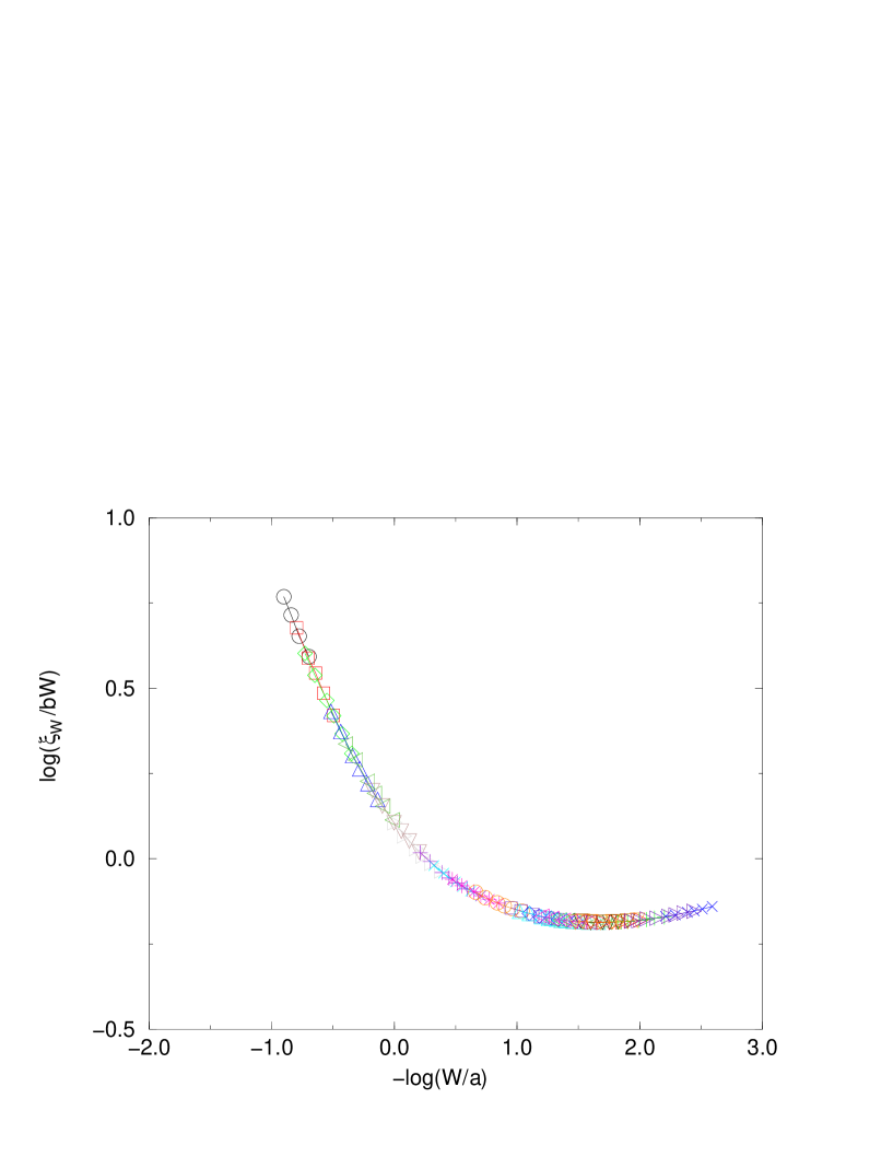
Figure 5: Same as fig. 2 for the diffusive phase in three dimensions. The frequency range is $0.5\leq\omega^{2}\leq 0.955$. $a$ and $b$ as functions of $\omega$ are reported in table 3

As can be seen from table 3, the parameters $a$ and $b$ increase in absolute value as $\omega$ is increased toward $\omega_{2}$, and diverge slowly. This implies an interesting behavior of the localization properties near $\omega_{2}$: Suppose that the asymptotic behavior of the scaling function $f$ in (11) for small argument is power like,

$$f(x)\sim x^{\beta}\ ,\qquad\mbox{for $x\rightarrow 0$}\ .$$ (19)

Taking a value of $\omega$ close to $\omega_{2}$, so that $a$ is very large, one finds from eqs. (11) and (19) that

$$\xi_{W}\sim W^{\beta}$$ (20)

for $W\ll a$. This behavior has to match the one observed at the lower edge of the anomalous localized phase, which implies the identity

$$\beta=\beta(\omega_{2})\sim 0.88\ .$$ (21)

The dependence on $W$ shown in (20) means that very close to the transition the system looks localized for small $W$ because $\xi_{W}/W$ is decreasing, before the crossover to the asymptotic linear growth of $\xi_{W}/W$. This scenario is corroborated by the minimum in the curve shown in fig. 5.

Since this is a conducting phase, it is instructive to compare the parameter $D$ with the conductivity $g$. The calculation of the latter from the Lyapunov spectrum may be achieved using eqs. (8) and (4). We remark that the dimensionless conductance $G$ calculated from (8) is sometimes called the transmission coefficient, since it is obtained by regarding the system as placed between ideal leads and providing $W^{d-1}$ channels which conduct energy between the leads. The precise dependence of $G$ on the channel transmissions is model dependent, and (8) reflects one possible choice [14].

The reason that $D$ gives a good estimate for $g$ in the diffusive phase is that the Lyapunov spectrum in this phase vanishes linearly at zero [15], and the spacing between the Lyapunov exponents changes slowly, as exemplified in fig. 6. This is in contrast with the Lyapunov spectrum in the low frequency range discussed below.

Figure 6: A typical Lyapunov spectrum in the diffusive phase, with the exponents decreasing linearly to zero. $\gamma_{i}$, $i=1,\ldots,144$ are the positive Lyapunov exponents for a bar of width 12, at $\omega^{2}=0.6$.

To see how $g$ and $D$ are related let us assume that the $W^{2}$ Lyapunov exponents are evenly spaced, with spacing $1/\xi_{W}$. The formula for the conductivity (8) involves a sharp cutoff at $\gamma_{n}\sim W$, so it basically counts the number of exponents smaller than $1/W$. Therefore we get $G\sim\xi_{W}/W$. Since $\xi_{W}\sim DW^{2}$ and $G=gW$, $g$ and $D$ are proportional. In table 3 we give the measured values of $g$. The agreement between $D$ and $g$ remains good throughout the diffusive phase.

3.4 The strongly conducting phase

In this subsection we describe the properties of the system for $\omega^{2}\leq\omega_{3}^{2}=0.45$.

We find that for very small $\omega$ short range disorder becomes irrelevant, and the vibration modes behave very similarly to modes of a pure system with a well-defined wave vector $k$ and an acoustic dispersion relation $\omega=c|k|$. Such modes exist even in one-dimensional systems, but are restricted to a band of width $W^{-1/2}$ around $\omega=0$. Similarly in three dimensions, although for any positive $\omega$ the transport is ultimately diffusive, there is a band of ballistic modes with a well defined wave vector near $\omega=0$, which disappears in the thermodynamic limit. The existence of this band may be simply understood as a consequence of the divergence of the mean free path $\ell$ as $\omega\to 0$. For any finite system there is a positive frequency $\omega_{b}$ where $\ell$ becomes larger than the system size, and for smaller frequency a wave propagates through the system with essentially no scattering.

Outside the ballistic band, and for $\omega\leq\omega_{3}$, the normal mode analysis of [5] shows that the modes experiences scattering which destroys the unique wave vector dependence. However, the absolute scale of the wave vector, the wavelength, is still well defined, and it is significantly larger than the lattice spacing. The wavelength is defined up to some width, which is commonly associated with the inverse of the mean free path.

The transport analysis of the present study reveals that a qualitative change in the structure of the Lyapunov spectrum occurs at $\omega_{3}$. In fig. 7 a typical Lyapunov spectrum of the low frequency phase is displayed, to be compared with fig. 6. The Lyapunov spectrum at small $\omega$ is characterized by the presence of large gaps; these obviously rule out the possibility of a description of the conductivity using a single parameter. The conductivity of the system depends sensitively on the system size, as well as the other parameters of the problem.

Figure 7: A typical Lyapunov spectrum in the strongly conducting, for a bar of width 12, at $\omega^{2}=0.2$ (compare with fig. 6.)

The origin of the gaps in the Lyapunov spectrum can be traced to the behavior of a pure system which is extended infinitely in the longitudinal direction. In such a system, for every longitudinal wave number $k_{\parallel}$, there are $W^{2}$ modes with

$$\omega_{n}^{2}=c_{s}^{2}(k_{\parallel}^{2}+k_{n}^{2})$$ (22)

where $k_{n}$, $1\leq n\leq W^{2}$ are the possible values of the transverse wave vector. These represent $W^{2}$ channels, which are perfectly conducting in the pure system. However, for a given $\omega$ one will have less then $W^{2}$ solutions since some of channels may be blocked, when the transverse vector is too large (transverse confinement). Therefore the conductivity of the pure system depends discontinuously on $\omega$: When $\omega$ is increased beyond the threshold values the conductivity jumps by an integer amount.

This picture describes quite accurately the conductance $G$ for small frequencies $\omega\ll\omega_{b}$. As $\omega$ is increased the Lyapunov spectrum is less well described by the one of an effective pure system, but gaps and irregularities in the spectrum persist up to $\omega_{3}$, reflecting a non-vanishing transverse confinement.

Consider the conductance $G$ as a function of $\omega$ for a fixed system size $W$. As just explained, for small $\omega$ system size the conductance is ballistic, and the value is proportional to the number of open channels, which is proportional to $(\omega W)^{2}$. This behavior persists as long as $W$ is smaller than the mean free path $\ell$. Since the mean free path diverges as $\ell\sim\omega^{-4}$ in three dimensions [6, 11], the crossover occurs at $\omega_{b}\sim W^{-1/4}$, therefore $G(\omega_{b})\sim W^{3/2}$.

Since the system is expected to be diffusive for any positive $\omega$, the dependence of $G$ on $W$ should change from the quadratic dependence of the ballistic range to an ultimately linear one, $G\sim gW$. If we assume a simple crossover from ballistic to diffusive behavior of $G$ when $W\sim\ell$, continuity of $G$ in $W$ implies that $(\omega_{b}W)^{2}\sim W^{3/2}\sim g(\omega_{b})W$, and the conductivity would diverge as $g(\omega)\sim\omega^{-2}$. However, the conductivity should diverge at the same rate as the mean free path, i.e., as $\omega^{-4}$. It follows then that there is a range in $W$ where $G$ grows stronger than linearly but weaker than quadratically, before the final diffusive behavior sets in.

These different behaviors and crossovers are represented in the conductance as measured numerically, and presented in fig. 8. The conductance at small $\omega$ is very well described by that of an effective pure system with sound speed $c_{s}=0.35$, which is between the two possible values for the elastic constant, $0.1$ and $1$ (recall that the masses were set to 1). The agreement is quantitative as is demonstrated in fig. 9, where the measured conductivity is shown against $\omega^{2}W^{2}$, and compared with that of the effective pure system. At the frequency range $\omega_{b}\leq\omega\leq\omega_{3}$ the functional form of $G$ is harder to describe. $G_{W}$ indeed grows faster than linearly and slower than quadratically, but as a result of the transverse effects discussed above, the growth rate is not monotonic and subject to sharp changes. Thus, we were unable to measure precisely the growth rate of $G$ as a function of $W$ for a fixed $\omega$. On the other hand it has been possible to measure the growth rate of the maximal value of $G$ for a fixed $W$

$$\max_{\omega}G_{W}(\omega)\sim W^{1.5}\ ,$$ (23)

which is the smallest possible growth rate, since $\max_{\omega}G_{W}(\omega)\geq G(\omega_{b})\sim W^{3/2}$. The ultimately linear growth of $G$ as a function of $W$ could not be observed in our numerics in this range for our system sizes.

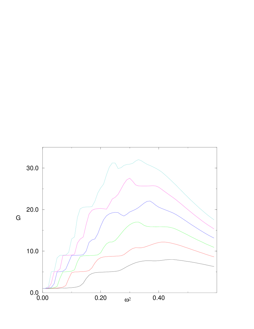
Figure 8: The conductance $G$ as function of the frequency squared $\omega^{2}$ for different bar widths. From bottom to top the widths are $W=6,\,8,\,10,\,12,\,14,\,16$. The dependence on $W$ for $\omega^{2}>0.45$ is linear.

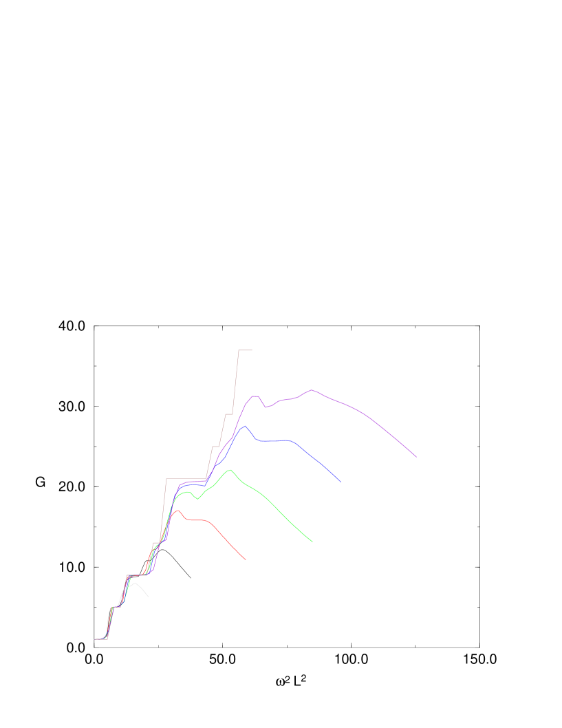
Figure 9: The same data as in fig. 8 but shown as a function as $\omega^{2}W^{2}$. The top curve is the result that would be obtained for a pure system with sound speed $c_{s}=0.35$.

4 Thermal conductivity in three dimensions

The results of the previous section can be used to calculate the overall heat conductivity of a three-dimensional disordered harmonic lattice, in the presence of a temperature gradient. The heat flow through a sample connected to two infinite ideal leads at different temperatures has been recently derived [16]. From this, the thermal conductivity $\kappa$ may be calculated, taking the temperature difference to be small, giving

$$\kappa={\hbar\over 2\pi}{1\over W}\int_{0}^{\infty}d\omega\omega\partial_{T}\eta_{T}(\omega)G(\omega)\ ,$$ (24)

where $G(\omega)$ is the frequency dependent transmission rate, discussed in the previous section, and $\eta_{T}(\omega)=1/(e^{\hbar\omega/T}-1)$. Below we use units such that Planck’s constant and Boltzmann’s constant are both equal to one.

The distribution function $\eta_{T}(\omega)$ which appears in  (24) diverges like $T/\omega$ for small $\omega$, and has an exponential cutoff at $\omega\sim T$. Hence for the purpose of a qualitative estimate we can replace $\eta_{T}(\omega)$ by $T/\omega$, cutting off the frequency integration at $\omega=CT$, with $C$ an order 1 constant. This approximation gives

$$\kappa\sim{1\over W}\int_{0}^{CT}d\omega G(\omega)\ .$$ (25)

Thus, as the temperature increases, modes with higher $\omega$ contribute to $\kappa$; if $CT$ is in the frequency range of one of the phases, then some of the modes of this phase contribute to $\kappa$, the phases of lower $\omega$ contribute fully, and those of higher $\omega$ do not contribute at all.

It follows that when $T\ll\omega_{3}$ only the strongly conducting phase should be taken into account. If the system is small enough so that $T\ll\omega_{b}$, the conductance is carried by ballistic modes, and eq. (25) gives

$$\kappa\sim WT^{3}\ ,$$ (26)

as in a perfect lattice. When $T>\omega_{b}$ this form is no longer valid, and scattering should be taken into account. Unfortunately, the numerical results provide limited information about the asymptotic behavior of $G$ in this range, and we are forced to make an ansatz about the form of $G$ which takes into account the numerical results and theoretical predictions, such as

$$G\sim\left\{\begin{array}[]{cl}\omega^{2}W^{2}&0<\omega<\omega_{b}\sim W^{-1/4}\\ W^{3/2}&\omega_{b}<\omega<\omega_{c}\sim W^{-1/8}\\ \omega^{-4}W&\omega_{c}<\omega<\omega_{3}\end{array}\right.\ .$$ (27)

This ansatz gives a linear dependence of $\kappa$ on $T$ in the intermediate frequency range, with a coefficient proportional to $W^{3/8}$ and a fast saturation at higher temperatures.

At temperatures greater or of the order of $\omega_{3}$ the contribution to $\kappa$ of the strongly conducting phase is therefore anomalous growing with the system size as $W^{3/8}$. The exponent of the anomaly should be considered as only indicative, but the contribution of the ballistic band itself already gives a $W^{1/4}$ anomaly. The divergence of the heat conductivity of the harmonic modes at low frequency is quite robust, and has been observed also in molecular simulations of glasses [4]. Nonlinear interaction are invoked to obtain heat conductivity which remains finite in the thermodynamic limit. This can be done phenomenologically by replacing the system size dependence of $\kappa$ by the inelastic mean free path.

In contrast, the contribution of the diffusive phase is quite simple:

$$\kappa_{\rm diffusive}\sim\int_{\omega_{3}}^{CT}D(\omega)\ ,$$ (28)

which gives Ohmic, system size independent, conductivity, increasing linearly at first, and saturating as $T\sim\omega_{2}$. This contribution, however, becomes negligible when the system size is taken to infinity. Finally the contribution of the localized phases to $\kappa$ decays exponentially in the system size, and these phases are insulating.

We also used eq. (24) to calculate $\kappa(T,W)$ directly from the numerical values of $G(\omega)$; the results are displayed in fig. 10, scaled with $W^{1/2}$. The integration over $\omega$ suppresses the finite size effects, and it can be seen that the $W^{1/2}$ scaling slightly overestimates the measured anomaly. As expected, one observes in fig. 10 a $T^{3}$ increase for small $T$, followed by a linear increase for intermediate $T$ and a saturation. A power law fit for the saturation yields an $W^{0.4}$ anomaly, but we regard this value as indicative only.

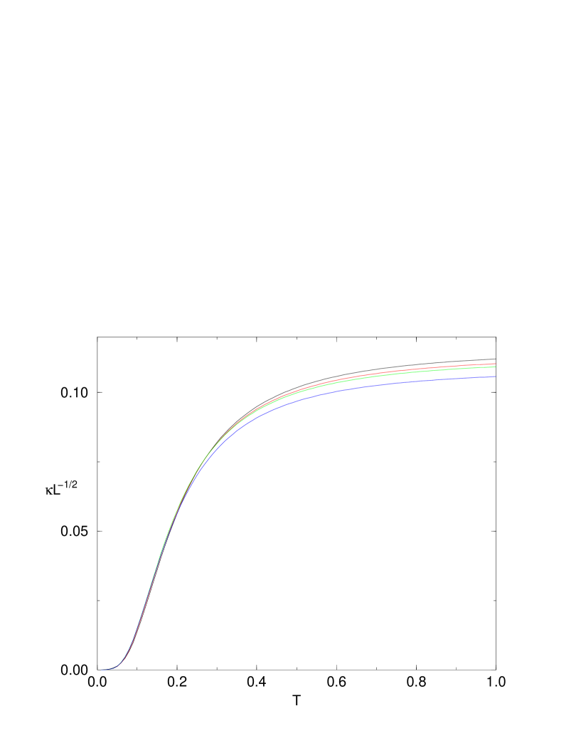
Figure 10: The thermal conductivity $\kappa$ of a cube of side $L$ divided by the square root of $L$, as a function of the temperature $T$, shown for different $L$s. The values of $L$ shown are (from to to bottom) 6, 8, 10, and 12.

5 Conclusions

We wish to comment on two central issues related to our model. First, in the scalar vibration model the delocalization transition is smoothed in the sense that there are two critical points, and there is a continuous change of the multifractal exponents near the transition. Moreover, far from the transitions one can observe the classical finite size scaling behavior similar to the Anderson scaling.

Our second principal conclusion is that the heat transport of modes of low frequency has some peculiarities probably related to the existence of a well defined wavelength. The low-temperature conductivity due to this band reproduces some of the experimental phenomena in glasses, such as a linear dependence on the temperature, and an eventual saturation (plateau). In recent papers [4], it has been argued that the heat transport in silicon glass is governed by harmonic modes; our model reproduces quite convincingly several of their results. In particular, there is no need to invoke non-linear processes such as two level systems to explain the temperature dependence of the heat conductivity. In all cases, however, the harmonic approximation yields a conductivity which diverges as some small power of the system size, and this feature must be corrected by the nonlinearity of the interaction.

The disordered lattice model is thus found to be a useful tool to study heat transport of glasses, and it will be very interesting to find out what will happen with a vector vibration field and with random masses.

Acknowledgments: We have profited from helpful discussions with I. Blanter, M. Büttiker, J.-P. Eckmann, G. Fagas, B. Galanti, A. Politi, and R. Zeitak. Z. O. thanks Jean-Pierre Eckmann for the invitation to the Département de Physique Théorique of the University of Geneva, which has been very useful for this work. This work has been supported in part by the Fonds National Suisse.

References

- [1] R.C. Zeller and R.O Pohl, Phys. Rev. B 4, 2029 (1971)
- [2] W.A. Philips J. Low temp. Phs. 7, 351(1972) and P.W. Anderson , B.I. Halperin and C.M. Varma Philos. Mag. 25,1(1975)
- [3] J.E. Grabner B. Golding and L.C. Allen Phys. Rev. B 34,5696 (1986)
- [4] P.B. Allen, J.L. Feldman, J. Fabian, and F. Wooten, cond-mat/9907132. J.L. Feldman, P.B. Allen, and S.R. Bickham, Phys. Rev. B 59, 3551 (1999).
- [5] B. Galanti and Z. Olami, cond-mat/9903392, cond-mat/9909227
- [6] S. John, H. Sompolinsky, and M.J. Stephen, Phys. Rev. B 27, 5592 (1983).
- [7] O. Gat, B. Galanti and Z. Olami, in preparation.
- [8] Q.-J. Chu and Z.-Q. Zhang, Phys. Rev. B 38, 4906 (1988).
- [9] A. MacKinnon and B. Kramer, Phys. Rev. Lett. 47 1546 (1981). J.-L. Pichard and G. Sarma, J. Phys. C. 14, L127, and L617.
- [10] T. Ohtsuki, K. Slevin and T. Kawarabayashi Ann. Phys. (Leipzig), 8, 655 (1999).
- [11] W. Schirmacher, G. Diezemann, C. Ganter Phys. Rev. Lett. 81, 136-139 (1998)
- [12] E. Gardner C. Itzykson, and B. Derrida, J. Phys. A. 17 (1984) 1093.
- [13] B. Kramer and A. MacKinnon, Rep. Prog. Phys. 56, 1469 (1993).
- [14] M. Büttiker, Y. Imry, R. Landauer, and S. Pinhas, Phys. Rev. B 31, 6207 (1985).
- [15] J.-L. Pichard and G. André Europhys. Lett. 2, 477 (1986).
- [16] M.P. Blencowe, Phys. Rev. B 59, 4992 (1999). L.G.C. Rego and G. Kirczenow, Phys. Rev. Lett. 81 232 (1998).