Possible Existence of an Extraordinary Phase in the Driven Lattice Gas

Abstract

We report recent simulation results which might indicate the existence of a new low-temperature “phase” in an Ising lattice gas, driven into a non-equilibrium steady state by an external field. It appears that this “phase”, characterized by multiple-strip configurations, is selected when square systems are used to approach the thermodynamic limit. We propose a quantitative criterion for the existence of such a “phase”. If confirmed, its observation may resolve a long-standing controversy over the critical properties of the driven Ising lattice gas.

1 Introduction

Nearly two decades ago, Katz, Lebowitz and Spohn introduced a seemingly trivial generalization of the Ising model: a lattice gas driven far from equilibrium by an external “electric” field, $E$ [1]. The motivations are twofold: the statistical mechanics of non-equilibrium systems and the physics of fast ionic conductors [2]. Since then, this model has provided a rich variety of surprises, showing how our intuition built on the foundations of equilibrium statistical mechanics fails when applied to non-equilibrium stationary states. Though some of its unusual properties are now understood, it continues to offer new surprises [3]. In this paper, we report recent simulation results which may be signals of a novel “phase”. If this new state is established, it would lead to a resolution of a long standing controversy concerning the critical properties. In the next section, we briefly describe the model and the disagreement between Marro, et. al. [8] and the Leung-Wang team[10]. Since the methods used in these two approaches are quite distinct, we explore, in Section III, the possibility that the discrepancies may lie in the existence of different types of ordering. In particular we introduce a new parameter which distinguishes the two low temperature “phases”. The systems used in our simulations are simple generalizations of the standard model – to include anisotropic interparticle interactions – so that the presence of the novel phase is more pronounced even for small lattices. The final section is devoted to some concluding remarks.

2 The driven lattice gas and its critical properties

The driven lattice gas is based on the Ising model [4, 5] with attractive nearest-neighbor interactions. In the spin language, it is a ferromagnetic Ising model with biased spin-exchange [6] dynamics. Since both the Onsager solution [7] and most simulations concern a system in two dimensions ($d=2$), we give a brief description of that model only. Each of the $L_{x}\times L_{y}$ sites of a square lattice (on a torus, i.e., with periodic boundary conditions: PBC) may be occupied by a particle or left vacant. A configuration of our system is specified by the occupation numbers $\{n_{i}\}$, where $i$ is a site label and $n$ is either 1 or 0. The interparticle attraction is modeled by the usual Hamiltonian: ${\cal H}=-4J\sum_{<i,j>}n_{i}n_{j}$, where $<i,j>$ are nearest-neighbor sites and $J>0$. In thermal equilibrium, a half filled system undergoes a second order phase transition, in the thermodynamic limit, at the Onsager temperature $T_{O}=(2.2692..)J/k_{B}$. To perform Monte Carlo simulations for this system, particles are allowed to hop to vacant nearest neighbor sites with probability $\min[1,e^{-\Delta{\cal H}/k_{B}T}]$, where $\Delta{\cal H}$ is the change in ${\cal H}$ after the particle-hole exchange. The deceptively simple modification introduced in [1] is to bias the hops along, say, the $y$ axis, so that the new rates are $\min[1,e^{-(\Delta{\cal H+}E\Delta y)/k_{B}T}]$. Locally, the effect of $E$ is identical to that due to gravity. However, due to the PBC, this modification cannot be accommodated by a (single-valued) Hamiltonian. Instead, the system settles into a non-equilibrium steady state with a non-vanishing global particle current. For temperatures above some finite critical $T_{c}$, the particle density in this state is homogeneous, while below $T_{c}$, the system displays phase segregation. Superficially, the driven system behaves like the equilibrium Ising model. With deeper probing, dramatic differences surface. For example, there is no question that its critical properties fall outside the Ising universality class. For recent reviews of this and other differences, we refer the interested reader to [3].

Focusing on critical properties here, let us review a long standing discrepancy between two sets of Monte Carlo results. While one set [10] shows data entirely consistent with field theoretic renormalization group predictions [11], another group [8] finds very different results, for which no viable theoretical analysis exists [12]. Technically, there are two serious differences between the simulation methods. In this section, we conjecture that different types of ordering may be responsible for the discrepancies. In view of the presence of “shape dependent” thermodynamics in the disordered phase of this system [13], we believe that the scenario pictured below is quite plausible. Let us begin with a brief review of the controversy.

Consider the (untruncated!) two point correlation function (in spin language): $G(x,y)\equiv\left\langle\left[2n(x,y)-1\right]\left[2n(0,0)-1\right]\right\rangle$, and its Fourier transform: $S(k,p)\equiv\sum_{x.y}G(x,y)e^{2\pi i\left(kx/L_{x}+py/L_{y}\right)}$, the structure factor. Due to the conserved dynamics, $S(0,0)\equiv 0$, so that non-trivial large distance properties are found in, e.g., $S(1,0)$ and $S(0,1)$. In equilibrium systems with square geometries ($L_{x}=L_{y}=L$), isotropy dictates that $S(1,0)=S(0,1)$, which approaches the static susceptibility in the thermodynamic limit for $T>$ $T_{O}$. As $T\rightarrow$ $T_{O},$ this quantity diverges (as $L^{\gamma/\nu}$ for finite systems at $T_{O}$). Below $T_{O}$, ordering is displayed as phase segregation, into a strip (of, say, a particle rich region) aligned with either the $x$- (or $y$-) axis, so that $S(0,1)$ (or $S(1,0)$) $\rightarrow L^{2}$. For the driven system, simulations [1] first revealed a discontinuity singularity ($S(1,0)>S(0,1)$) in the disordered phase and showed further that, at low $T$, phase segregation occurs only into “vertical” strips ($S(1,0)=O(L^{2}),$ $S(0,1)=O(1)$). Since these structure factors are related to (the inverse of) diffusion co-efficients in a continuum theory, these observations formed the basis for the study of a model where, first, the diffusion co-efficients are anisotropic, and second, more importantly, only one of these co-efficients vanishes as $T\rightarrow$ $T_{c}$ [11]. This approach is also consistent with subsequent simulations [14] showing that, while $S(1,0)$ diverges as $T\rightarrow$ $T_{c}$, $S(0,1)$ remains $O(1)$ throughout the transition. A serious consequence of this “strongly anisotropic” behavior is that parallel and transverse lengths and momenta scale with different powers ($p_{y}\sim p_{x}^{1+\Delta}$, $\Delta=1$ in mean field theory) in the critical region. Analogues of this unusual property exist in equilibrium systems [15]. When fluctuations are taken into account via renormalization group methods [11], the upper critical dimension ($d_{c}$) is found to be $5$, while anomalous scaling modifies $\Delta$ to $2$ in $d=2.$ A more subtle result is that one set of exponents retains the classical values.

Now, in order to /measure/ critical properties through simulations, with some accuracy, it is crucial to exploit finite size scaling methods [16]. Systems with various $L$’s are used, and the quality of data collapse serves as an indicator of the presence of scaling. Given the highly anisotropic scaling of lengths, the analysis would be much simplified if samples obeying $L_{y}\sim L_{x}^{3}$ are used. This route is pioneered and followed in one of the studies [10]. More importantly, the order parameter used is closely related to $S(1,0)$, so that it is sensitive to the presence of a single domain (i.e., one vertical strip, regardless of the system size). Also measured are cumulant ratios associated with $S(1,0)$. All data thus obtained display good collapse, using a set of exponents that is entirely consistent with those predicted by the renormalization group [11]. In another set of studies [8], only square samples are used. Furthermore, the order parameter used is

$$m\equiv\sqrt{\left\langle M_{y}^{2}\right\rangle-\left\langle M_{x}^{2}\right\rangle}$$ (1)

where $M_{x(y)}^{2}\equiv L^{-2}\sum_{y(x)}\left[\sum_{x(y)}\left\{2n_{i}-1\right\}\right]^{2}$. Note that, if the ordered phase consists of a single vertical strip, then $m$ provides information about its average density. However, configurations with vertically aligned multiple strips also contribute to $m.$ The conclusion is that, e.g., $\beta\simeq\frac{1}{4}$, contradicting the field theory results [8].

3 A possible novel phase

It should be quite alarming that two sets of simulations lead to drastically different conclusions, unless we allow the possibility that the “ordered” states in the two studies are not the same. Considering $m$ is not sensitive to the presence of multiple strips, we conjecture the following.

• In the thermodynamic limit, the low temperature state in systems with square geometry ($L_{x}=L_{y}$) is characterized by multiple strips, with a nontrivial distributions of widths.

In other words, we believe that there is no long range order (which would lead to a single-strip state) while strip-strip correlations are controlled by a finite correlation length. For short, we will use a more picturesque term: “stringy phase.”

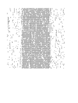
Figure 1: A typical “stringy” configuration vs. a typical single strip one. (See text for system parameters.)

Significantly, the existence and behavior of such configurations were first noted in [8]. Indeed, these authors wrote: “The system was never seen to escape from (these multiple-strip) states… and we had to manipulate some system configurations for $L=50$ to create artificial one-strip states…”. For $L\geq 100$ systems, they were “unable to observe the decay (of these multiple-strip states) toward one-strip states…” The conclusion was that multiple states are “metastable” with exceedingly long life times.

Another source for our conjecture comes from simulation studies of a driven lattice gas with anisotropic interparticle interactions ($J_{x}\neq J_{y}$) [17]. Though typical configurations are disordered/ordered(single strip) for high/low temperatures, there is a significant range of $T$ where the system appears to be “stringy.” In Fig.1, we show such a configuration at $T=0.80$, found in a $90\times 90$ lattice with $3J_{x}=J_{y}/3=J$, driven with saturation $E$. (Here, as in the following, $T$ is given in units of $T_{O}$.) In contrast, the single strip configuration was obtained with $T=0.70$. To be more precise, the “stringy” states may be characterized by two properties: (a) the densities in each column (i.e., along the drive) are bi-modally distributed, yet (b) $S(1,0)$ remains small [18]. An example is provided in Fig.2. While the column densities begin to develop a double peak around $T\sim 0.90$, the structure factor displays an inflection point at $T\sim 0.70$ (which is also where the fluctuations in $S(1,0)$ reach a maximum). Note that bi-modal column densities correspond to $m>0$. Yet, in this range ($0.75\lesssim T\lesssim 0.95$), the typical configurations are far from being single-stripped. To show that multiple-strip states are not simply metastable, we ran simulations starting from a completely ordered (single-strip) state. Unlike in the previous study [8], we do observe the split-up into multiple strip states. In Fig.3, we show a time trace of 3500 measurements (700K MCS) of $S(k,0)$, $k=1,2,3$, which are sensitive to the presence of $k$-strip domains. Note that $S(1,0)$ is often smaller than $S(2,0)$ and sometimes even smaller than $S(3,0)$, as shown in the inset. As a check, we made three separate runs of this length and observed the same type of behavior. Our conclusion is that, despite being started in a completely ordered state, the system evolves towards a “stringy” state. In other words, the probability to find the system in multiple strip configurations can be considerable.

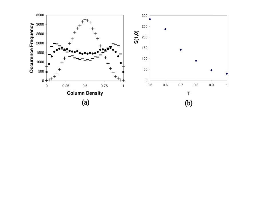
Figure 2: (a) Histogram for column densities at $T=0.80$[$-$], $0.90$[$\bullet$], $2.0$[$+$], and (b) $S(1,0)$ vs. $T$ in a $30\times 30$ lattice with $3J_{x}=J_{y}/3=J$, driven with saturation $E$.

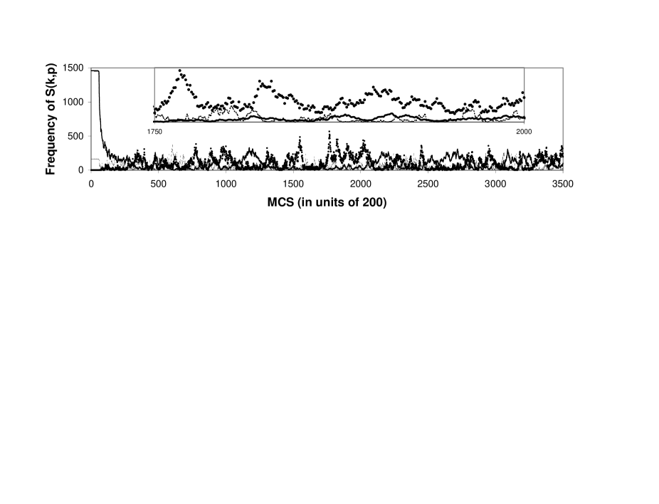
Figure 3: Time trace of $S(k,0)$, $k=1$ [solid line], $2$ [$\bullet$], $3$, [dashed line], for a $60\times 60$ lattice at $T=0.85$, driven with saturation $E$. Inset: magnified view of a portion.

In order to make quantitative statements about the “stringy state”, we introduce the ratio:

$${\cal R}\equiv L^{d}\frac{G(0,L/2)}{S(1,0)}$$ (2)

for a system in $d$ dimensions. The numerator is a measure of “long range order” along the $y$-axis, while the denominator detects the presence of a single strip. In particular, we are interested in the behavior of ${\cal R}$, as $L\rightarrow\infty$, when the system is in various states.

Far in the disordered phase, the two-point correlation decays as $r^{-d}$ [19]. Thus, $G(0,L/2)\rightarrow O(L^{-d})$, while $S(1,0)$ remains $O(1)$. On the other hand, deep in the ordered phase $G\rightarrow O(1)$ while $S\rightarrow O(L^{d})$. As a result, we expect

$${\cal R}\rightarrow O(1)$$ (3)

for both high and low temperatures. In between, a finite system makes a transition, either through a “stringy phase” or directly into the ordinary ordered state (as in the equilibrium case). In the latter scenario, the results of the renormalization group analysis [11] should hold: $G(0,r)\rightarrow r^{-[d-2+\Delta]/(1+\Delta)}$ and $S(k,0)\rightarrow k^{-2}$. Thus, for simulations in $d=2$, we conclude that ${\cal R}$ decreases with $L:$

$${\cal R}\rightarrow L^{-2/3}.$$ (4)

In sharp contrast, for a stringy state, ordering has set in along $y$ (so that $G(0,L/2)\rightarrow O(1)$) but complete phase segregation in $x$ is yet to take hold (so that $S(1,0)\rightarrow O(1)$). The consequence is an increasing ${\cal R}:$

$${\cal R}\rightarrow L^{d}.$$ (5)

which is a function of $L.$ The drastic differences between these asymptotic properties (3, and 4 vs. 5) should be detectable through simulations. As a final remark, we note that, for the equilibrium Ising model, ${\cal R}$ decreases exponentially as $L^{2}e^{-L/\xi}$ for $T>T_{c}$, while for $T\lesssim T_{c}$, ${\cal R}$ is $O(1)$.

Turning to Monte Carlo data, we find that the evidence in favor of stringy states is quite strong, at least for the $L$’s we can access. In particular, using models with $J_{x}=J/3$ and $J_{y}=3J$ under saturation drive, we collected data from a number of systems with $L\in\left[10,90\right]$. The runs are up to 800K MCS long, with both random and ordered initial conditions. In Fig.4, we show a plot of ${\cal R}$ vs. $L^{2}$, for various temperatures. For $T=0.85$ and $0.90$, this ratio appears to be proportional to $L^{2}$. Meanwhile, its behavior is consistent with ${\cal R}\rightarrow O(1)$ at both higher and lower $T$’s. We believe that these results support the presence of a “stringy phase”.

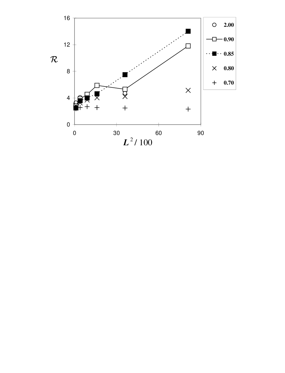
Figure 4: Correlation-Structure Factor ratio ${\cal R}$ for systems with $\alpha=3$ and saturation drive, plotted against $L^{2}.$ The legend refers to the temperatures of the various runs.

Of course, this “phase” may be just a mirage in the landscape of a giant crossover. In the absence of analytic results, we can never be certain of its existence, since all simulations are based on finite $L$. Nevertheless, if future simulations continue to support ${\cal R}\propto O(L^{2})$, then it behooves us find a sound analytic basis for such a state. To conclude this section, we conjecture further. As $L$ increases further, the stringy phase will persist at lower and lower temperatures, so that it is the only low temperature state, for square systems, in the limit $L\rightarrow\infty$. However, if the thermodynamic limit is approached through systems obeying $L_{y}\propto L_{x}^{3}$, the low temperature phase will consist of the ordinary, single-domain state. If this conjecture turns out to be true, then an avenue is opened for the resolution of the controversy over critical properties.

4 Concluding remarks

In this short paper, we explored the possibility that the low temperature phase of the driven lattice gas depends on the geometry of the system. For square systems, we conjecture that a new, “stringy” phase is the only ordered state in the limit $L\rightarrow\infty$. On the other hand, if an Ising-like, ordered state with a single domain is desired, then the “unusual” thermodynamic limit, with rectangular systems obeying $L_{\|}\propto L_{\bot}^{3}$, must be used. For finite square geometries, we have some Monte Carlo evidence for the presence of a “stringy” state: multiple strips of high/low density regions. The system appears to be “ordered” in the direction parallel to the drive, but the strips are of varying widths and multiplicities. Specifically, as $T$ is lowered, the disordered, homogeneous phase gives way to this multi-strip state for a sizable range of $T$, before settling into the fully phase segregated, single domain state at lower temperatures.

Many open questions, besides those mentioned above, naturally arise. More quantitative analyses can be carried out, in order to better characterize this “stringy” state. For example, we could measure the distribution of strip-widths, or compile histograms for both the structure factors and the correlations. Once a clearer picture emerges, assuming such a state still exists, we should attempt to develop a reliable field theory. Certainly, the order parameter of such a theory, $m$ in Eqn. (1), is necessarily quite different from the one for an equilibrium Ising lattice gas. Hopefully, renormalization group methods can be applied, a nontrivial fixed point can be obtained, and its associated critical properties can be computed. Until then, to compare field-theoretic predictions with simulation data from the Marro studies makes as much sense as “comparing apples with oranges.”

5 Acknowledgments

It is a pleasure to dedicate this article to Joel Lebowitz, a co-author of this model. Over the years, we have benefitted from numerous conversations with him, not to mention all the encouragements when we run into apparent dead-ends. Also, we are grateful to J. Hager for help with simulations, as well as G.L. Eyink and U.C. Täuber for illuminating discussions. This research was supported in part by a grant from US National Science Foundation through the Division of Materials Research and a supplement from the Research Experience for Undergraduates program.

References

- [1] S. Katz, J. L. Lebowitz and H. Spohn, Phys. Rev. B 28, 1655 (1983); J. Stat. Phys. 34, 497 (1984).
- [2] See, e.g., S. Chandra, Superionic Solids. Principles and Applications (North Holland, Amsterdam 1981).
- [3] See, e.g., B. Schmittmann and R. K. P. Zia, Phase Transitions and Critical Phenomena, Vol. 17, edited by C. Domb and J. L. Lebowitz (Academic, London, 1995) and B. Schmittmann and R. K. P. Zia, Phys. Rep. 301, 45 (1998).
- [4] Ising, Z. Physik 31, 253 (1925). A more recent treatment is, e.g.,
- [5] C.N. Yang and T.D. Lee, Phys. Rev. 87, 404 (1952); and T.D. Lee and C.N. Yang, Phys. Rev. 87, 410 (1952).
- [6] K. Kawasaki, Ann. Phys. 61, 1 (1970).
- [7] L. Onsager, Phys. Rev. 65, 117 (1944) and Nuovo Cim. 6, (Suppl.) 261 (1949).
- [8] J.L. Vallés and J. Marro, J. Stat. Phys. 49, 89 (1987). For references to more recent studies by Marro and collaborators, see [9]
- [9] J. Marro and R. Dickman, Nonequilibrium Phase Transitions in Lattice Models (Cambridge, 1999).
- [10] K.-t. Leung, Phys. Rev. Lett. 66, 453 (1991) and Int. J. Mod. Phys. C3, 367 (1992); J. S. Wang, J. Stat. Phys., 82, 1409 (1996). See also K.-t. Leung and R.K.P. Zia, J. Stat. Phys. 83, 1219 (1996).
- [11] H.K. Janssen and B. Schmittmann, Z. Phys. B64, 503 (1986); K-t. Leung and J.L. Cardy, J. Stat. Phys. 44, 567 and 45, 1087 (Erratum) (1986).
- [12] P. L. Garrido, F. de los Santos and M. A. Munoz, Phys. Rev. E57, 752 (1998) proposed an alternative formulation. However, for , they conclude that “the resulting critical theory is the equilibrium one, i.e., model B, for the () transverse directions…” Applying this theory to simulation data, which are obtained in systems, does not seem viable.
- [13] F.J. Alexander and G.L. Eyink, Phys. Rev. E57, R6229 (1998) and G.L. Eyink,J.L. Lebowitz and H. Spohn, J. Stat. Phys. 83, 385 (1996).
- [14] R.K.P. Zia and T. Blum, in Scale Invariance, Interfaces and Non-equilibrium Dynamics, eds. M.Droz, A.J. McKane, J. Vannimenus, and D.E. Wolf, (Plenum, N.Y., 1995).
- [15] R.M. Hornreich, M. Luban, and S. Shtrikman, Phys. Rev. Lett. 35, 1678 (1975); D. Mukamel, J. Phys. A10, L24 (1977); and S.M. Bhattacharjee and J. F. Nagle, Phys. Rev. A 31:3199 (1985).
- [16] See, e.g., V. Privman, Finite Size Sacling and Numerical Simulations of Statistical Systems, (World Scientific, Singapore, 1990).
- [17] L.B. Shaw, B. Schmittmann, and R.K.P. Zia, J. Stat. Phys. 95, 981 (1999), cond-mat/9807057.
- [18] L.B. Shaw, Monte Carlo and Series Expansion Studies of the Anisotropic Driven Ising Lattice Gas Phase Diagram MS thesis, Virginia Polytechnic Institute and State University (May, 1999).
- [19] M. Q. Zhang, J. -S. Wang, J. L. Lebowitz and J.L. Valles, J. Stat. Phys. 52, 1461 (1988); P. L. Garrido, J. L. Lebowitz, C. Maes and H. Spohn, Phys. Rev. A42, 1954 (1990). R.K.P. Zia, K. Hwang, K-t. Leung, and B. Schmittmann, in Computer Simulation Studies in Condensed Matter Physics V, eds. D.P. Landau, K.K. Mon, and H.-B. Schüttler, (Springer, Berlin, 1993a).