Critical properties of the metal-insulator transition
in anisotropic systems

Abstract

We study the three-dimensional Anderson model of localization with anisotropic hopping, i.e., weakly coupled chains and weakly coupled planes. In our extensive numerical study we identify and characterize the metal-insulator transition by means of the transfer-matrix method. The values of the critical disorder $W_{c}$ obtained are consistent with results of previous studies, including multifractal analysis of the wave functions and energy level statistics. $W_{c}$ decreases from its isotropic value with a power law as a function of anisotropy. Using high accuracy data for large system sizes we estimate the critical exponent as $\nu=1.62\pm 0.07$. This is in agreement with its value in the isotropic case and in other models of the orthogonal universality class.

1 Introduction

We study numerically the problem of Anderson localization And58 in three-dimensional (3D) disordered systems with anisotropic hopping. Previous studies using the transfer-matrix method (TMM) LiSEG89 ; ZamLES96a ; PanE94 , multifractal analysis (MFA) MilRS97 and recently energy-level statistics (ELS) MilR98 ; MilRS99a showed that an MIT exists even for very strong anisotropy. The values of the critical disorder $W_{c}$ were found to decrease by a power law in the anisotropy, reaching zero only for the limiting 1D or 2D cases. The main goal of the present paper is to determine the critical exponent $\nu$ of this second order phase transition with high accuracy. It is generally assumed that $\nu$ only depends on general symmetries, described by the universality class, but not on microscopic details of the sample KraM93 . Thus, anisotropic hopping should not change $\nu$. Recent highly accurate TMM studies report $\nu=1.54\pm 0.08$ Kin94 , $\nu=1.58\pm 0.06$ SleO99a , $\nu=1.61\pm 0.07$, and $\nu=1.54\pm 0.03$ CaiRS99 for isotropic systems of the orthogonal universality class. But for anisotropic systems of weakly coupled planes, $\nu=1.3\pm 0.1$ and $\nu=1.3\pm 0.3$ was found ZamLES96a . We found in a recent high precision ELS study $\nu=1.45\pm 0.2$ MilRS99a for the same model. To clarify this situation, we compute the localization length by means of the TMM with high accuracy for large system sizes and apply a finite-size scaling (FSS) analysis which takes into account corrections to the usual one-parameter scaling ansatz SleO99a . The resulting value of the critical exponent $\nu=1.62\pm 0.07$ confirms the recent high accuracy estimates. Thus the anisotropic Anderson model belongs to the same universality class as the isotropic model.

Another interesting aspect of anisotropic hopping beside the question of universality is the connection to experiments which use uniaxial stress to tune disordered Si:P or Si:B systems across the MIT PaaT83 ; StuHLM93 ; BogSB99 ; WafPL99 . While applying stress, the distance between the atomic orbitals reduces, the electronic motion becomes alleviated, and the system changes from insulating to metallic. Thus, although the explicit dependence of hopping strength on stress is material specific and in general not known, it is reasonable to relate uniaxial stress in a disordered system to an anisotropic Anderson model with increased hopping between neighboring planes.

In the experiments, a large variation of the value of the critical exponent $\nu$ has been observed with suggested values ranging from 0.5 PaaT83 over 1.0 WafPL99 , 1.3 StuHLM93 , up to 1.6 BogSB99 . Possibly this “exponent puzzle” StuHLM93 is due to other effects in the experiments such as electron-electron interaction BogSB99 or sample inhomogeneities StuHLM93 ; RosTP94 ; StuHLM94 which are usually ignored in the original formulation of Anderson localization. Furthermore, the extrapolation of finite-temperature conductivity data down to temperature $T=0$ is open to debate and should perhaps be replaced WafPL99 ; ItoWOH99 by application of the dynamical scaling approach BelK94 . Another interesting question is, whether applying uniaxial stress is equivalent to changing the dopant concentration. We note that for non-universal properties such as the value of the conductivity, it was shown that stress and concentration tuning lead to different $T$ dependencies close to the MIT WafPL99 .

2 The anisotropic Anderson model of localization

We use the standard Anderson Hamiltonian And58

$${\bf H}=\sum_{i}\epsilon_{i}|i\rangle\langle i|+\sum_{i\neq j}t_{ij}|i\rangle\langle j|\quad$$ (1)

with orthonormal states $|i\rangle$ corresponding to electrons located at sites $i=(x,y,z)$ of a regular cubic lattice with periodic boundary conditions. The potential energies $\epsilon_{i}$ are independent random numbers drawn from the interval $[-W/2,W/2]$. The disorder strength $W$ specifies the amplitude of the fluctuations of the potential energy. The hopping integrals $t_{ij}$ are non-zero only for nearest neighbors and depend on the three spatial directions, thus $t_{ij}$ can either be $t_{x}$, $t_{y}$ or $t_{z}$. We study two possibilities of anisotropic transport: (i) weakly coupled planes with

$$t_{x}=t_{y}=1\quad,\quad t_{z}=1-\gamma$$ (2)

and (ii) weakly coupled chains with

$$t_{x}=t_{y}=1-\gamma\quad,\quad t_{z}=1\quad.$$ (3)

This defines the strength of the hopping anisotropy $\gamma\in[0,1]$. For $\gamma=0$ we recover the isotropic case, $\gamma=1$ corresponds to independent planes or chains. Note that uniaxial stress would be modeled by weakly coupled chains after renormalization of the hopping strengths such that the largest $t$ is set to one in equation (3).

3 Transfer-matrix method in anisotropic systems

We study the localization length $\lambda$, describing the exponential decay of the wave function on long distances. We compute it using the TMM KraM93 ; PicS81a ; MacK81 for quasi-1D bars of cross section $M\times M$ and length $L\gg M$. The stationary Schrödinger equation ${\bf H}\Psi=E\Psi$ is rewritten in a recursive form:

$${\Psi_{i+1}\choose\Psi_{i}}={\left(\begin{array}[]{cc}(E{\bf 1}-{\bf H}_{i})/t_{b}&{\bf-1}\\ {\bf 1}&{\bf 0}\end{array}\right)}{\Psi_{i}\choose\Psi_{i-1}}={\bf T}_{i}{\Psi_{i}\choose\Psi_{i-1}}.$$ (4)

$\Psi_{i}$, ${\bf H}_{i}$, and ${\bf T}_{i}$ are wave function, Hamiltonian matrix, and transfer matrix of the $i$th slice, respectively. Unit and zero matrices are denoted by ${\bf 1}$ and ${\bf 0}$ and $t_{b}$ is the hopping integral along the bar axis. We consider the band center $E=0$. Given an initial condition ${\Psi_{1}\choose\Psi_{0}}$ equation (4) allows a recursive construction of the wave function in the bar geometry by adding more and more slices. $\lambda(M,W)$ is then obtained from the smallest Lyapunov exponent of the product ${\bf T}_{L}{\bf T}_{L-1}\cdots{\bf T}_{2}{\bf T}_{1}$ of transfer matrices MacK83 , where the length $L$ of the bar is increased until the desired accuracy of $\lambda$ is achieved. With increasing cross section of the bar the reduced localization length $\Lambda_{M}=\lambda(M,W)/M$ decreases for localized states and increases for extended states. Thus it is possible to determine the critical disorder at which $\Lambda_{M}$ is constant from plots of $\Lambda_{M}$ versus $M$.

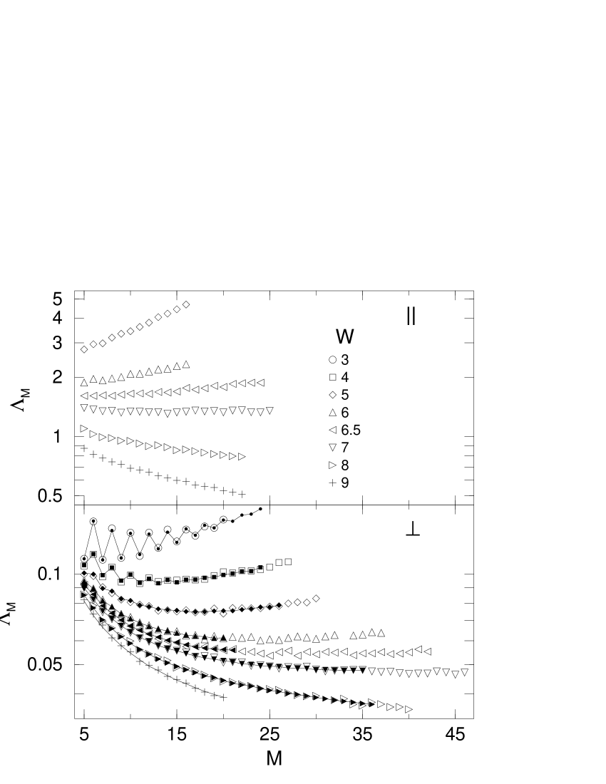
Figure 1: Reduced localization length for coupled planes with $\gamma=0.96$ for parallel (top) and perpendicular (bottom) orientation of the transfer-matrix bar. Accuracy is 1% (large symbols) or 0.2% (small filled symbols connected by lines to guide the eye).

For the anisotropic systems there are two possible orientations of the axis of the quasi-1D bar: parallel and perpendicular to the coupled planes or chains. The localization lengths in the perpendicular direction are smaller than in the parallel direction by a factor of about $1-\gamma$ for coupled planes and $(1-\gamma)^{2}$ for chains ZamLES96a . Nevertheless, the critical disorder $W_{c}$ should not depend on the orientation of the bar ZamLES96a . For strong anisotropies $\gamma\geq 0.9$ this is difficult to verify numerically, as can be seen for the case of weakly coupled planes in figure 1. For the parallel orientation of the bar we find the usual critical behavior of $\Lambda_{M}$ as described above. We deduce a critical disorder $W_{c}\approx 7$ for this case. But for a perpendicular orientation of the bar the behavior of $\Lambda_{M}$ versus $M$ is different as can be seen in the bottom part of figure 1. There are two striking features. First, $\Lambda_{M}$ oscillates for small $W$ and $M$ between smaller values for odd and larger values for even $M$. Second, the characteristics of $\Lambda_{M}$ as function of $M$ changes from localized (with positive slope) at small $M$ to extended (with negative slope) at larger $M$ for $W<7$. Let us consider for instance the data for $W=6$. For $M<11$ $\Lambda_{M}$ decreases with $M$, which is typical for localized states. Up to $M\approx 25$ the data still decrease, but the slope tends to zero. For $M>25$ it starts to increase, indicating extended behavior. Therefore one has to extend the calculation at least to $M=35$ to find the correct critical disorder in this case. For smaller $M$, $W_{c}$ would be systematically underestimated even when applying the FSS procedure. We remark that, e.g., the computation of the data point for $W=8$, system size $M=36$, and accuracy of 0.2% takes several weeks on a 400MHz Pentium II machine.

Figure 2: DOS for $M$ weakly coupled planes of size $M\times M$ with $W=3$ and $\gamma=0.96$ for an odd and an even $M$.

We attribute these features of $\Lambda_{M}$ at least partially to a structured density of states (DOS) $\rho(E)$ at these large $\gamma$ and relatively small $W$. We show an example in figure 2. The structure comes from very small ($M\times M$) planes in the bar which are very weakly coupled in the perpendicular direction. The coupling between the planes is so small for $\gamma>0.9$, that $\rho(E)$ is nearly equal to the DOS of an ensemble of uncoupled 2D systems MilRS97 . In such small 2D systems the relatively weak disorder is not sufficient to completely smear out the peaks in the DOS of the ordered system. Thus, at $E=0$ there is a peak for even but a dip for odd system sizes as can be seen in figure 2. In our opinion, for the TMM in perpendicular orientation, $M$ has to be at least so large that all the finite size structure in $\rho(E)$ has vanished in order to get reliable results. For the TMM in parallel orientation, smaller $M$ are sufficient, since the planes or chains extend along the bar so that the DOS is smoothened.

4 Computation of the critical properties at the MIT

4.1 Anisotropy dependence of $W_{c}$

Depending on the quality of our available data, we compute the critical disorder with different methods. The results are shown in figures 3 and 4. Particularly for the perpendicular orientation we estimate $W_{c}$ from plots of $\Lambda_{M}$ versus $M$ as in figure 1. As described above, a constant behavior of $\Lambda_{M}$ for large system sizes indicates $W_{c}$. For data without the described features due to a structured DOS, i.e., in the parallel orientation, we plot the disorder dependence of $\Lambda_{M}$ for several system sizes as in figure 5. The transition is indicated by a crossing point of the $\Lambda_{M}(W)$ curves. We use FSS for high quality data as described in the next subsections. Our results for $W_{c}$ are in good agreement with results from ELS MilR98 ; MilRS99a and MFA MilRS97 . The power-law dependence on anisotropy $W_{c}=16.5(1-\gamma)^{\beta}$ is confirmed. Using all data from MFA MilRS97 , ELS, and the present TMM, we find $\beta=0.25\pm 0.05$ and $\beta=0.60\pm 0.08$ for coupled planes and chains, respectively. The latter deviates slightly from the CPA result ZamLES96a $\beta=0.5$.

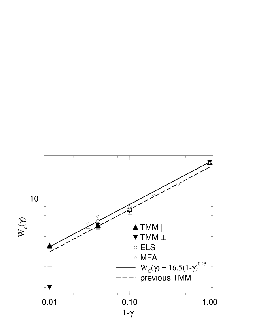
Figure 3: Anisotropy dependence of $W_{c}$ for coupled planes as computed by TMM in parallel ($\|$) and perpendicular ($\perp$) direction, previously by MFA MilRS97 and recently by ELS MilRS99a . We also added a fit to TMM data of Ref. ZamLES96a (dashed line). Note the large systematic error explained in section 3 for the TMM in perpendicular direction at $\gamma=0.99$.

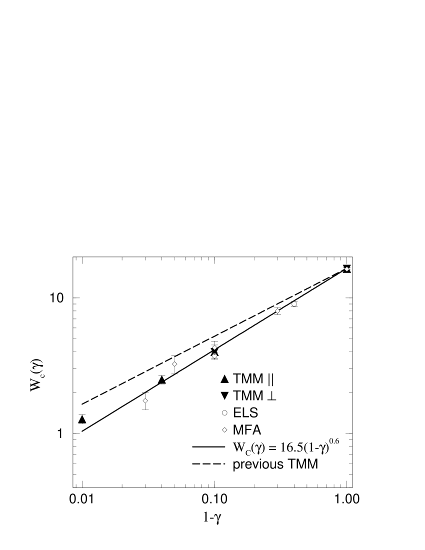
Figure 4: Anisotropy dependence of $W_{c}$ for coupled chains as computed by TMM in parallel ($\|$) and perpendicular ($\perp$) direction, previously by MFA MilRS97 and recently by ELS MilRS99a . We also added a fit to TMM data of Ref. ZamLES96a (dashed line).

4.2 Finite-size scaling

The MIT in the Anderson model of localization is expected to be a second-order phase transition BelK94 ; AbrALR79 . It is characterized by a divergent correlation length $\xi_{\infty}(W)=C|W-W_{c}|^{-\nu}$, where $\nu$ is the critical exponent and $C$ is a constant KraM93 . To construct the correlation length of the infinite system $\xi_{\infty}$ from finite size data $\Lambda_{M}$ ZamLES96a ; KraM93 ; PicS81a ; MacK81 , the one-parameter scaling hypothesis Tho74 is employed,

$$\Lambda_{M}=f(M/\xi_{\infty})\quad.$$ (5)

All $\Lambda_{M}$ are expected to collapse onto a single scaling curve $f$, when the system size is scaled by $\xi_{\infty}$. In a system with MIT such a scaling curve consists of two branches corresponding to the localized and the extended phase. One might determine $\nu$ from fitting $\xi_{\infty}$ obtained by a FSS procedure MacK83 . But a higher accuracy can be achieved by fitting directly the raw data MacK83 . We use fit functions SleO99a which include two kinds of corrections to scaling: (i) nonlinearities of the disorder dependence of the scaling variable and (ii) an irrelevant scaling variable with exponent $-y$. Specifically, we fit

$$\Lambda_{M}=\tilde{f}_{0}(\chi_{\rm r}M^{1/\nu})+M^{-y}\tilde{f}_{1}(\chi_{\rm r}M^{1/\nu})\quad,$$ (6)

$$\tilde{f}_{n}=\sum_{i=0}^{n_{\rm r}}a_{ni}\chi_{\rm r}^{i}M^{i/\nu}\quad,\quad\chi_{\rm r}(w)=w+\sum_{n=2}^{m_{\rm r}}b_{n}w^{n}$$ (7)

with $w=(W_{c}-W)/W_{c}$ and $a_{ni}$ and $b_{n}$ expansion coefficients. Choosing the orders $n_{\rm r}$ and $m_{\rm r}$ of the expansions larger than one, terms with higher order than linear in the $W$ dependence appear. This allows to fit a wider $W$ range around $W_{c}$ than with the previously used linear fitting Kin94 . The linear region is usually very small. The second term in equation (6) describes the systematic shift of the crossing point of the $\Lambda_{M}(W)$ curves Kin94 ; SleO99a visible, e.g., in figure 5 and its inset. This correction term vanishes for large system sizes, since the irrelevant exponent $y>0$.

For the nonlinear fit, we use the Levenberg-Marquardt method SleO99a ; PreFTV92 as in Ref. MilRS99a . It minimizes the $\chi^{2}$ statistics, measuring the deviation between model and data under consideration of the error of the data points. We estimate the quality of the fit by the goodness of fit parameter $Q$ PreFTV92 . It considers $\chi^{2}$ and the number of data points and fit parameters. For reliable fits it should lie in the range $0.01<Q<1$ PreFTV92 . We check the confidence intervals obtained from the Levenberg-Marquardt routine by a Monte Carlo and a bootstrap method PreFTV92 . Additionally, we test whether the fitted values of $W_{c}$, $\nu$, and $y$ are compatible when using different expansions of the fit function, i.e., different orders $n_{\rm r}$ and $m_{\rm r}$ MilRS99a .

4.3 Determination of $\nu$

We estimate $\nu$ for coupled planes with strong anisotropy $\gamma=0.9$, where we have the most accurate data. A parallel orientation of the transfer-matrix bar is used in order to avoid the problems discussed in section 3. Compared to the perpendicular direction, the convergence of the TMM is much slower and the computing time to achieve a certain accuracy increases remarkably. We computed $\Lambda_{M}$ up to $M=17$ with $0.07\%$ accuracy for $8.1\leq W\leq 9$, for $W=8$, 9.1, and 9.2 the accuracy is $0.14\%$. As we show in figure 5 we find a clear signature of an MIT, a crossover from increasing to decreasing behavior of $\Lambda_{M}$ with growing $M$ when disorder changes from 8 to 9.2. The lines for constant $M$ do not cross exactly in a single point. In the inset, a small systematic shift is clearly visible. Thus, we include the second term of equation (6) when fitting the data. All fits reported in table 1 describe the data very well. This is expressed by the large values of $Q>0.7$ and can also be seen in figure 5 where we show the data and the fit functions for an exemplary set of parameters $n_{\rm r},m_{\rm r}$. The corresponding scaling function and scaling parameter are displayed in figure 6 and its inset. All data collapse almost perfectly onto a single curve with two branches. In connection with the divergent $\xi_{\infty}$, this clearly indicates the MIT. We also tried to use smaller orders of the expansions than in table 1, but then it was not possible to fit the data in the whole $W$ interval with the desired high quality.

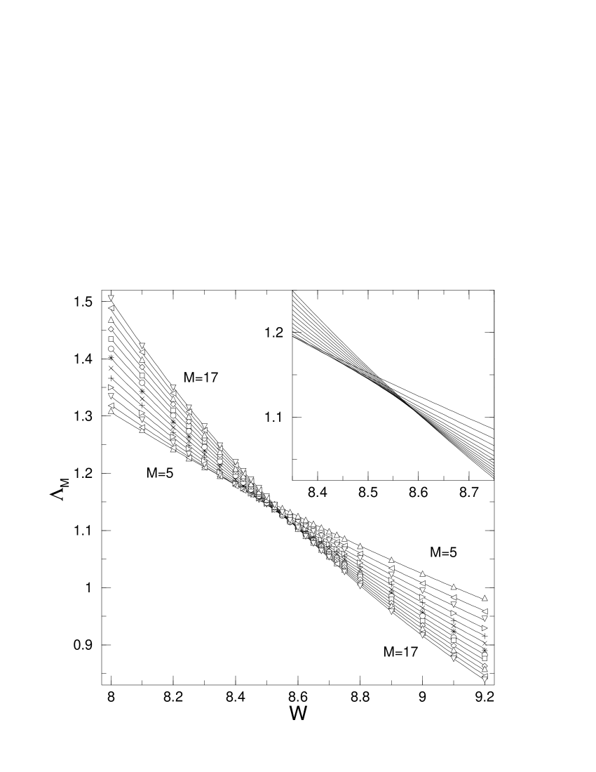
Figure 5: Reduced localization length for coupled planes with $\gamma=0.9$ and $M=5,6,\ldots,17$. The lines are fits of the data according to equations (6) and (7) with $n_{\rm r}=3$ and $m_{\rm r}=2$. In the inset we enlarge the central region without the data points to show the shift of the crossing point.

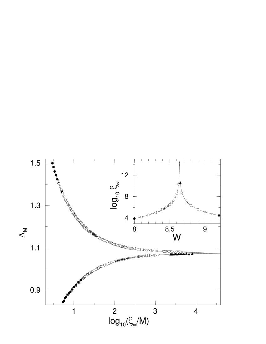
Figure 6: Scaling function and scaling parameter, shown in the inset, corresponding to the fit in figure 5. The symbols distinguish different $W$ values of the scaled data points.

	$M$	$n_{\rm r}$	$m_{\rm r}$	$\chi^{2}$	$Q$	$W_{c}$	$\nu$	$y$
$\vartriangle$	$5\cdots 17$	3	1	306.2	0.789	$8.62\pm 0.01$	$1.65\pm 0.04$	$1.56\pm 0.27$
$\vartriangleleft$	$5\cdots 17$	2	3	309.8	0.745	$8.64\pm 0.01$	$1.59\pm 0.04$	$1.31\pm 0.23$
$\triangledown$	$5\cdots 17$	3	2	303.0	0.815	$8.63\pm 0.01$	$1.64\pm 0.04$	$1.51\pm 0.27$
$\vartriangleright$	$5\cdots 17$	3	3	300.7	0.829	$8.63\pm 0.01$	$1.64\pm 0.04$	$1.55\pm 0.27$
$\blacktriangle$	$7\cdots 17$	3	1	218.6	0.995	$8.64\pm 0.03$	$1.66\pm 0.07$	$1.34\pm 0.77$
$\blacktriangleleft$	$7\cdots 17$	2	3	211.7	0.998	$8.65\pm 0.02$	$1.60\pm 0.05$	$1.34\pm 0.47$
$\blacktriangledown$	$7\cdots 17$	3	2	209.2	0.999	$8.64\pm 0.02$	$1.62\pm 0.07$	$1.38\pm 0.51$
$\blacktriangleright$	$7\cdots 17$	3	3	208.9	0.998	$8.65\pm 0.03$	$1.59\pm 0.12$	$1.24\pm 0.58$

Table 1: Fit parameters and estimates for $W_{c}$ and $\nu$ with 95% confidence intervals from fitting $\Lambda_{M}$ for coupled planes with $\gamma=0.9$. The symbol in the first column is used in figure 7.

When comparing the spreading of the fitted $W_{c}$ and $\nu$ values in table 1 with their confidence intervals for the case that all system sizes are used in the fits (open symbols), the error estimates appear to be slightly too small. The 95% confidence intervals of the smallest and largest $W_{c}$ value do not overlap. We thus conclude $W_{c}=8.63\pm 0.02$. In figure 7 we show the fitted $\nu$ values and their confidence intervals together with results from our recent ELS study MilRS99a using the same fit method. The characters A to E denote ELS results from different combinations of $W$ and $M$ intervals. Despite the high accuracy of the data of 0.2% to 0.4% for large system sizes up to $M=50$ and large $Q$ values, the results for $\nu$ scatter strongly. The 95% confidence interval apparently do not describe the correct error in this case. But for the TMM data, the error estimate for $\nu$ seems to be appropriate. We emphasize the importance of having very accurate data for high system sizes as prerequisite to obtain reliable critical exponents. Furthermore, it is necessary to compare the results of different fits to get reasonable error estimates.

In order to test for a possible systematic trend in the finite size behavior, we have repeated the fits neglecting the smallest system sizes $M=5,6$. This is denoted by filled symbols in table 1. The results do not change, only the error increases. We summarize our result for the critical exponent as $\nu=1.62\pm 0.07$. This is different from $\nu=1.3\pm 0.1$ and larger than $\nu=1.3\pm 0.3$ obtained previously from data with an accuracy of about 2% for system sizes up to $M=15$ and $17$ for the parallel and perpendicular direction ZamLES96a . Since we use more accurate data with slightly larger system sizes we expect our result to be more reliable. Furthermore, $\nu\approx 1.6$ is in good agreement with high accuracy TMM studies for the isotropic case Kin94 ; SleO99a ; SleO97 . For comparison, we have added the results of Ref. SleO99a to figure 7. In our recent ELS study MilRS99a we obtained $\nu=1.45\pm 0.2$. As in other ELS studies Hof98 ; ZhaK97 , the critical exponent is smaller than deduced from highly accurate TMM data. However, within the error bars, that result is consistent with our present finding. In Ref. MilRS99a a trend towards larger $\nu$ was found when the data from smaller samples were neglected. A further increase of $\nu$ can be presumed if the system size could be increased further. We believe, that for large enough system sizes TMM and ELS will give the same results.

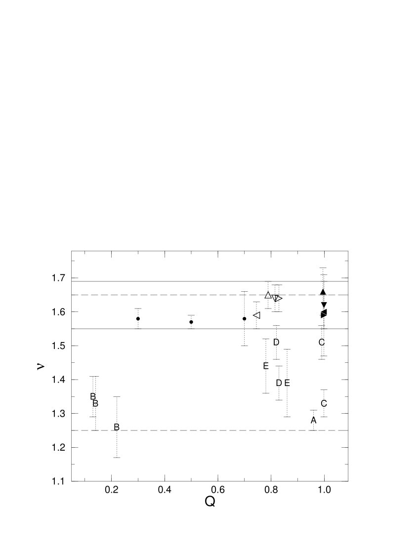
Figure 7: $\nu$ and its 95% confidence intervals from the fits of the $\Lambda_{M}$ data as reported in table 1. Large characters denote fits of ELS data from Ref. MilRS99a . The $\bullet$ data indicate results of Ref. SleO99a for the isotropic case $\gamma=0$. Solid and dashed lines indicate the error bounds for the present result $\nu=1.62\pm 0.07$ and the ELS result MilRS99a $\nu=1.45\pm 0.2$, respectively.

5 Summary

We have studied the metal-insulator transition in the 3D Anderson model of localization with anisotropic hopping. We used TMM together with FSS analysis to characterize the MIT. Our results confirm the existence of an MIT for anisotropy $\gamma<1$ for weakly coupled planes and weakly coupled chains and the power law decay of the critical disorder with increasing anisotropy found in studies using TMM ZamLES96a , MFA MilRS97 , and recently by ELS MilR98 ; MilRS99a . In these anisotropic systems there are two possible orientations of the transfer matrix bar. We have shown that the critical disorder $W_{c}$ is, as expected, the same for both possibilities. But we remark that for strong anisotropy $\gamma$ very large system sizes are necessary for the perpendicular orientation in order to find the correct $W_{c}$. This is in part due to the small size of the weakly coupled planes or chains in the bar which results in a structured DOS.

For the case of weakly coupled planes with $\gamma=0.9$ and parallel orientation we computed $\Lambda_{M}$ with 0.07% accuracy for system widths up to $17\times 17$. Using a method to fit the data SleO99a which considers corrections to scaling due to an irrelevant scaling variable and nonlinearities in the disorder dependence of the scaling variables we have deduced a critical exponent $\nu=1.62\pm 0.07$. This is clearly larger than $\nu=1.3\pm 0.1$ obtained previously ZamLES96a for the same system. Since this result was obtained from less accurate data ($\approx$ 2%) and slightly smaller system sizes, we believe that the previous error estimate is too small. Even from highly accurate ELS data (0.2% to 0.4%) and system sizes up to 50 the error estimate is twice as large: $\nu=1.45\pm 0.2$ MilRS99a . We have shown that large system sizes and high accuracies are necessary to determine the critical exponent reliably. Our result is in good agreement with other high accuracy TMM studies for the orthogonal universality class Kin94 ; SleO99a ; CaiRS99 ; SleO97 . These numerical estimates of $\nu$ seem to converge towards $\nu\approx 1.6$. Experimentally it is of course even more difficult to determine the exponent $\nu$ of the Anderson transition. Recent attempts of dynamical temperature scaling have shown that the statistical accuracy of the experimental data is less than in the numerical studies WafPL99 ; ItoWOH99 ; BogSB99b , but there also seems to be a trend towards larger values of $\nu$ PaaT83 ; WafPL99 .

- (1) P. W. Anderson, Phys. Rev. 109, 1492 (1958).
- (2) Q. Li, C. Soukoulis, E. N. Economou, and G. Grest, Phys. Rev. B 40, 2825 (1989).
- (3) I. Zambetaki, Q. Li, E. N. Economou, and C. M. Soukoulis, Phys. Rev. Lett. 76, 3614 (1996), cond-mat/9704107.
- (4) N. Panagiotides and S. Evangelou, Phys. Rev. B 49, 14122 (1994).
- (5) F. Milde, R. A. Römer, and M. Schreiber, Phys. Rev. B 55, 9463 (1997).
- (6) F. Milde and R. A. Römer, Ann. Phys. (Leipzig) 7, 452 (1998).
- (7) F. Milde, R. A. Römer, and M. Schreiber, submitted to Phys. Rev. B (1999), cond-mat/9909210.
- (8) B. Kramer and A. MacKinnon, Rep. Prog. Phys. 56, 1469 (1993).
- (9) A. MacKinnon, J. Phys.: Condens. Matter 6, 2511 (1994).
- (10) K. Slevin and T. Ohtsuki, Phys. Rev. Lett. 82, 382 (1999), cond-mat/9812065.
- (11) P. Cain, R. A. Römer, and M. Schreiber, Ann. Phys. (Leipzig) 8, SI-33 (1999), cond-mat/9908255.
- (12) M. A. Paalanen and G. A. Thomas, Helv. Phys. Acta 56, 27 (1983).
- (13) H. Stupp, M. Hornung, M. Lakner, O. Madel, and H. v. Löhneysen, Phys. Rev. Lett. 71, 2634 (1993).
- (14) S. Bogdanovich, M. P. Sarachik, and R. N. Bhatt, Phys. Rev. Lett. 82, 137 (1999).
- (15) S. Waffenschmidt, C. Pfleiderer, and H. v. Löhneysen, (1999), cond-mat/9905297.
- (16) T. F. Rosenbaum, G. A. Thomas, and M. A. Paalanen, Phys. Rev. Lett. 72, 2121 (1994).
- (17) H. Stupp, M. Hornung, M. Lakner, O. Madel, and H. v. Löhneysen, Phys. Rev. Lett. 72, 2122 (1994).
- (18) K. M. Itoh, M. Watanabe, Y. Outuka, and E. E. Haller, Ann. Phys. (Leipzig) 8, 631 (1999).
- (19) D. Belitz and T. R. Kirkpatrick, Rev. Mod. Phys. 66, 261 (1994).
- (20) J.-L. Pichard and G. Sarma, J. Phys. C: Solid State Phys. 14, L127 (1981).
- (21) A. MacKinnon and B. Kramer, Phys. Rev. Lett. 47, 1546 (1981).
- (22) A. MacKinnon and B. Kramer, Z. Phys. B 53, 1 (1983).
- (23) E. Abrahams, P. W. Anderson, D. C. Licciardello, and T. V. Ramakrishnan, Phys. Rev. Lett. 42, 673 (1979).
- (24) D. J. Thouless, Phys. Rep. 13, 93 (1974).
- (25) W. H. Press, B. P. Flannery, S. A. Teukolsky, and W. T. Vetterling, Numerical Recipes in FORTRAN, 2nd ed. (Cambridge University Press, Cambridge, 1992).
- (26) K. Slevin and T. Ohtsuki, Phys. Rev. Lett. 78, 4083 (1997), cond-mat/9704192.
- (27) E. Hofstetter, Phys. Rev. B 57, 12763 (1998), cond-mat/9611060.
- (28) I. K. Zharekeshev and B. Kramer, Phys. Rev. Lett. 79, 717 (1997), cond-mat/9706255.
- (29) S. Bogdanovich, M. P. Sarachik, and R. N. Bhatt, Ann. Phys. (Leipzig) 8, 639 (1999).