Supercooled Liquids and Glasses

Walter Kob
Institute of Physics, Johannes-Gutenberg University, D-55099 Mainz, Germany

1 Introduction

Glasses are materials that are much more common in our daily life than one might naively expect. Apart from the obvious (inorganic) glasses, such as wine glasses, bottles and windows, we also have the organic (often polymeric) glasses, such as most plastic materials (bags, coatings, etc.). In the last few years also metallic glasses have come to our daily (St. Andrews) life since they are used, apart from many other applications, in the head of golf clubs. In view of this widespread use of these materials it might be a bit surprising to learn that glasses are not very well understood from a microscopic point of view and that even today very basic questions such as “What is the difference between a liquid and a glass?” cannot be answered in a satisfactory way. In the present lecture notes we will discuss some of the typical properties of supercooled liquids and glasses and theoretical approaches that have been used to describe them. Since unfortunately it is not possible to review here all the experiments on glasses and theoretical models to explain them we will discuss here only some of the most basic issues and refer the reader who wants to learn more about this subject to other review articles and textbooks [1].

In the following section we will review some of the basic phenomena that are found in supercooled liquids and glasses. Subsequently we will discuss the theoretical approaches to describe the dynamics of these systems, notably the so-called mode-coupling theory of the glass transition. This will be followed by the presentation of results of computer simulations to check to what extend this theory is reliable. These results are concerned with the equilibrium dynamics. If the temperature of the supercooled liquid is decreased below a certain value, the system is no longer able to equilibrate on the time scale of the experiments, i.e. it undergoes a glass transition. Despite the low temperatures the system still shows a very interesting dynamics the nature of which is today still quite unclear. Therefore we will present in the final part of these lecture notes a brief discussion of this dynamics and its implication for the (potential) connection of structural glasses with spin glasses.

2 Supercooled Liquids and the Glass Transition

In this section we will discuss some of the properties of supercooled liquids and some of the phenomena of the glass transition.

If a liquid is cooled from high temperatures below its melting point $T_{m}$ one expects it to crystallize at $T_{m}$. However, since the crystallization process takes some time (critical nuclei have to be formed and have to grow) it is possible to supercool most liquids, i.e. they remain liquid-like even below $T_{m}$. Some liquids can be kept in this metastable state for a long time and thus it becomes possible to investigate their properties experimentally. For reasons that will become clear below, such liquids are called good glass-formers. It is found that with decreasing temperature the viscosity $\eta$ of these systems increases by many orders of magnitude. In order to discuss this strong temperature dependence it is useful to define the so-called glass transition temperature $T_{g}$ by requiring that at $T_{g}$ the viscosity is $10^{12}$ Pa s, which corresponds roughly to a relaxation time of 100 seconds (reminder: water at room temperature has a viscosity around $10^{-3}$ Pa s). In figure 1 we show the temperature dependence of $\log(\eta)$ for a variety of glass-formers as a function of $T/T_{g}$. From that plot we see that the viscosity does indeed increase dramatically when temperature is decreased. Furthermore we recognize that this temperature dependence depends on the material in that there are substances in which $\eta(T)$ is very close to an Arrhenius law, i.e. are almost straight lines, and other substances in which a pronounced bend in $\eta(T)$ is found. In order to distinguish these different temperature dependencies Angell are coined the terms “strong” and “fragile” glass-formers for the former and latter, respectively [3].

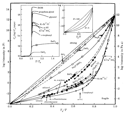
Figure 1: Main figure: Viscosity of different glass-formers as a function of $T_{g}/T$, where $T_{g}$ is the glass transition temperature. Left inset: Temperature dependence of the specific heat, normalized to its value for the crystall, for different glass-formers. From reference [2], with permission.

The strong temperature dependence which is found in $\eta(T)$ is not a unique feature of the viscosity. If other transport quantities, such as the diffusion constant, or relaxation times are measured, it is found that they show a similar temperature dependence as the viscosity. On the other hand if thermodynamic quantities, such as the specific heat, or structural quantities, such as density or the structure factor, are measured, they show only a relatively mild dependency in the same temperature interval, i.e. they vary between 10% and a factor of 2-3.

Equipped with these experimental facts one can now ask the main question of glass physics: What is the reason for the dramatic slowing down of the dynamics of supercooled liquids without an apparent singular behavior of the static quantities? Although this question seems to be a very simple one it has not been possible up to now to find a completely satisfying answer to it. One obvious response is to postulate the existence of a second order phase transition at temperatures below $T_{g}$. Then the slowing down could be explained as the usual critical slowing down observed at the critical point. Although such an explanation is from a theoretical point of view very appealing it suffers one big drawback, namely that so far it has not been possible to identify an order parameter which characterizes this phase transition or a characteristic length scale which diverges. Thus despite the nice theoretical concept the phase transition idea is not able to provide a satisfactory explanation for the slowing down of the dynamics.

Things look much better for a different theoretical approach, the so-called mode-coupling theory (MCT) of the glass transition, which we will discuss in mode detail below. This theory is indeed able to make qualitative and quantitative prediction for the time and temperature dependence of various quantities and experiments and computer simulations have shown that many of these predictions are true [4]. However, before we discuss the predictions of MCT we return to the temperature dependence of the viscosity or the relaxation times. From figure 1 it is clear that for every material there will be a temperature at which the relaxation time of the system will exceed by far any experimental time scale. This means that it will not be possible to probe the equilibrium behavior of the system below this temperature. If the system is continously with a given cooling rate from a high temperature to low temperatures there will exist a temperature $T_{g}^{\prime}$ at which the typical relaxation time of the system is comparable to the inverse of the cooling rate. Hence in the vicinity of this temperature the system will fall out of equilibrium and become a glass. (Note that the other glass transition temperature that we have introduced above, $T_{g}$, is basically the value of $T_{g}^{\prime}$ if one assumes that the relaxation time is on the order of 100 s.) This glass transition is accompanied by the freezing of those degrees of freedom which lead to a relaxation of the system, such as the motion of the particles beyond the nearest neighbor distance. Since below $T_{g}^{\prime}$ these degrees of freedom are no longer able to take up energy the specific heat shows a drop at $T_{g}^{\prime}$, as it can be seen in the left inset of figure 1. Note that empirically it is found that the fragile glass-formers show a large drop in the specific heat whereas the strong glass-formers show only a small one. Note, however, that this correlation is just an empirical one (and it does not hold strictly) and apart from hand-waving arguments it is not understood from a theoretical point of view. The same is also true for the distinction between strong and fragile glass-formers. So far it is not clear what the essential features in a Hamiltonian are that make the system strong or fragile, i.e. is this the range of the interaction, the coordination number, etc.

At the beginning of this section we mentioned that the dynamics of glass-forming liquids becomes slow when they are cooled below the melting temperature. However, it is not a necessary condition for a slow dynamics that the temperature is below $T_{m}$. E.g. silica has a melting temperature around 2000K and a glass transition temperature around 1450K [5]. From Figure 1 it becomes obvious that at $T_{m}=T_{g}/0.725$ the viscosity is already on the order of $10^{7}$Pa s! Thus it is clear that slow dynamics has nothing to do with the system being supercooled, or in other words: for the glass transition the melting temperature is a completely irrelevant quantity. Despite this fact we will in the following continue to talk about “supercooled” liquids, following the usual (imprecise) usage of this term.

We now turn our attention to the MCT , the theory we have briefly mentioned earlier. Here we will give only a very sketchy idea about this theory and refer the reader who wants to learn more about it to the various review articles on MCT [4, 6]. In the MCT the quantities of interest are the correlation functions between the density fluctuations of the particles. If we denote by ${\bf r}_{j}(t)$ the position of the particle $j$ at time $t$ the density fluctuations are given by [7]

$$\delta\rho({\bf q},t)=\sum_{j=1}^{N}\exp(i{\bf q}\cdot{\bf r}_{j}(t))\quad,$$ (1)

where ${\bf q}$ is the wave-vector. From this observable one can calculate the so-called intermediate scattering function $F(q,t)$ which is given by

$$F(q,t)=\frac{1}{N}\langle\delta\rho(-{\bf q},t)\delta\rho({\bf q},0)\rangle\quad.$$ (2)

Here the angular brackets stand for the thermodynamic average. The relevance of the function $F(q,t)$ is given by the fact that it can be directly measured in neutron and light scattering experiments. From a theoretical point of view this correlation function is important since many theoretical descriptions of (non-supercooled) liquids are based on it, or its time and space Fourier transforms [7].

Using the Mori-Zwanzig projection operator formalism [7] it is now possible to derive exact equations of motion for the $F(q,t)$. These are of the form

$$\ddot{F}(q,t)+\Omega^{2}(q)F(q,t)+\int_{0}^{t}d\tau M(q,\tau)\dot{F}(t-\tau)=0.$$ (3)

Here $\Omega^{2}(q)$ is given by $q^{2}k_{B}T/mS(q)$, where $m$ is the mass of the particles and $S(q)$ is the static structure factor, i.e. $S(q)=F(q,0)$. The function $M(q,\tau)$ is called the memory function and formally exact expression exist for it. However, because of their complexity, these formal expressions are basically useless for a real calculation and thus in MCT one approximates $M(q,\tau)$ by a quadratic form of the density correlators. In particular it is found that $M(q,t)$ is given by

$$M(q,t)=\frac{1}{2(2\pi)^{3}}\int d{\bf k}V^{2}(q,k,|{\bf q}-{\bf k}|)F(k,t)F(|{\bf q}-{\bf k}|,t)$$ (4)

where the vertex $V^{2}$ is given by

$$V^{2}(q,k,|{\bf q}-{\bf k}|)=\frac{n}{q^{2}}\left(\frac{{\bf q}}{q}\left[{\bf k}c(k)+({\bf q}-{\bf k})c(|{\bf q}-{\bf k}|)\right]\right)$$ (5)

and the so-called direct correlation function $c(k)$ can be expressed via the structure factor by $(S(k)-1)/nS(k)$, where $n$ is the particle density. Thus we see that within MCT the static structure factor determines the vertex $V^{2}$, which in turn determines the memory function for the time dependent correlation function. Or in other words: The statics determine the dynamics.

Note that similar equations of motion as the one for $F(q,t)$ exist for the incoherent intermediate scattering function, $F_{s}(q,t)$. This correlation function is given by

$$F_{s}(q,t)=\frac{1}{N}\left\langle\sum_{j}^{N}\exp(i{\bf q}\cdot({\bf r}_{j}(t)-{\bf r}_{j}(0))\right\rangle\quad,$$ (6)

i.e. it is just the self (or diagonal) part of $F(q,t)$. Also this time correlation function is important since it can be measured in scattering experiments.

Instead of making at this point a detailed discussion of the properties of the solutions of these MCT equations we will postpone this discussion to section 4 where we will make a detailed comparison of the prediction of MCT with the results of computer simulations. The only thing that we mention already now is that it has been shown that at long times there are two types of solution of the MCT equations. The first one is the solution $\lim_{t\to\infty}F(q,t)=0$. This solution is the only one at high temperature and it corresponds to the physical situation that the system is ergodic, i.e. all time correlation functions decay to zero. (Note that temperature enters though the temperature dependence of the static structure factor $S(q)$). The second solution has the property that $\lim_{t\to\infty}F(q,t)>0$ and it occurs only below a critical temperature $T_{c}$. Since in this case the correlation functions do not decay to zero even at long times, the system is no longer ergodic, i.e. it is a glass. Thus within the MCT the system undergoes a glass transition at $T_{c}$. MCT now makes an asymptotic expansion of the dynamics around this critical point, i.e. it treats the quantity $\epsilon=(T_{c}-T)/T_{c}$ as a small parameter. Hence all the predictions of the theory are, strictly speaking, only valid very close to $T_{c}$ and it is difficult to say a priori how far away from $T_{c}$ they are still useful. However, our experience of analyzing data has shown that the theory can be used for values $\epsilon$ as large as 0.5 or so [4], thus with respect to this the situation seems to be much better than the case of critical phenomena.

3 On Computer Simulations

In the last few decades computer simulations have been shown to be a very powerful tool to gain insight into the behavior of statistical mechanic systems and thus can be considered to be a very useful addition to experiments and analytical calculations. Present days computer codes for such simulations are usually quite complex and thus we are not going to discuss the various tricks used in such simulations but refer the reader to some text books and the lecture of K. Kremer in this school [8, 9].

Simulations of supercooled liquids and glasses pose special problems for computer simulations since at low temperatures the relaxation times are large, see the previous section, and thus the simulations have to be done for many (microscopically small!) time steps. Fortunately it is usually not necessary to use very large system sizes, a few hundred to a few thousand particles are adequate for most cases, and thus all the computer resources are spend to simulate the system over a time span which is as large as possible. Therefore present day state of the art calculations extend over 10-100 million time steps which corresponds to several month up to several years of CPU time on a top of the line processor. Note that despite this effort the length of such a runs corresponds to only about $10^{-7}$ seconds, since each time step is on the order of $10^{-15}$ seconds. However, it should be noted that the time window of these simulations, i.e. 7-8 decades, exceeds the one of most experimental techniques, such as neutron or light scattering. A more extensive discussion of advantages and disadvantages of computer simulations of supercooled liquids and glasses and references to the original literature can be found in Refs. [10].

We now discuss some of the details of the simulations whose results will be discussed in the next few sections. As mentioned in the previous paragraph the main issue of computer simulations of supercooled liquids is to investigate the system at a temperature which is as close as possible to the glass transition temperature, i.e. in that temperature range where the relaxation times of the system are large. Therefore it is advisable to use a system that can be simulated as efficiently as possible. Hence many investigations have been done for so-called “simple liquids”, i.e. systems in which the interaction between the particles is isotropic and short ranged. One possible example for such a system is a one-component Lennard-Jones liquid. The main drawback of this system is that it is prone to crystallization, i.e. something which in this business has to be avoided at all costs. Therefore it has become quite popular to study binary liquids, since the additional complexity of the system is sufficient to prevent crystallization, at least on the time scale accessible to todays computer simulations.

The system we study is hence a binary Lennard-Jones liquid and in the following we will call the two species of particles “type A” and “type B” particles. The interaction between two particles of type $\alpha$ and $\beta$, $\alpha,\beta\in\{{\rm A,B}\}$, is thus given by: $V_{\alpha\beta}=4\epsilon_{\alpha\beta}[(\sigma_{\alpha\beta}/r)^{12}-(\sigma_{\alpha\beta}/r)^{6}]$. The values of the parameters $\epsilon_{\alpha\beta}$ and $\sigma_{\alpha\beta}$ are given by $\epsilon_{AA}=1.0$, $\sigma_{AA}=1.0$, $\epsilon_{AB}=1.5$, $\sigma_{AB}=0.8$, $\epsilon_{BB}=0.5$, and $\sigma_{BB}=0.88$. This potential is truncated and shifted at a distance $\sigma_{\alpha\beta}$. In the following we will use $\sigma_{\rm AA}$ and $\epsilon_{\rm AA}$ as the unit of length and energy, respectively (setting the Boltzmann constant $k_{\rm B}=1.0$). Time will be measured in units of $\sqrt{m\sigma_{\rm AA}^{2}/48\epsilon_{\rm AA}}$, where $m$ is the mass of the particles.

In the following we will study two types of dynamics for this system: A Newtonian dynamics (ND) and a stochastic dynamics (SD). The reason for investigating the ND is that this is a realistic dynamics for an atomic liquid. Thus it is possible to study at low temperatures the interaction of the phonons with the relaxation dynamics of the system. On the other hand the SD is a good model for a colloidal suspension in which the particles are constantly hit by the (much smaller) particles of the bath. In such systems the phonons are strongly damped and thus such a dynamics is one way to “turn off” the phonons. Hence, by comparing the results of the two types of dynamics it becomes possible to find out which part of the dynamics is universal, i.e. does not depend on the microscopic dynamics, and which part is non-universal.

In both types of simulations the number of A and B particles were 800 and 200, respectively. The volume of the simulation box was kept constant at a value of $(9.4)^{3}$, which corresponds to a particle density of around 1.2. The temperatures used were 5.0, 4.0, 3.0, 2.0, 1.0, 0.8, 0.6, 0.55, 0.5, 0.475, 0.466, 0.456, and 0.446. At each temperature the system was thoroughly equilibrated for a time span which significantly exceeded the typical relaxation times of the system at this temperature. At the lowest temperatures this took up to 40 million time steps. As we will see, the relaxation times for the SD are, at low temperatures, significantly longer than the ones for the ND. Therefore we used in all cases the ND to equilibrate the sample and used the SD only for the production runs. For the ND we used at low temperatures a time step of 0.02, whereas for the SD a smaller one, 0.008, was needed in order to avoid systematic errors in the equilibrium quantities. In order to improve the statistics of the results we averaged over eight independent runs.

4 The Equilibrium Relaxation Dynamics

In this section we will discuss the relaxation dynamics of the system in equilibrium. The main emphasis will be to find out to what extend this dynamics depends on the microscopic dynamics and which aspects of it can be understood within the framework of the mode-coupling theory.

Before we study the dynamical properties of the system it is useful to have a look at its static properties. In section 2 we have mentioned that in the supercooled regime thermodynamic quantities and structural quantities show only a weak temperature dependence. That this is the case for the present system as well is demonstrated in figure 2, where we show the static structure factor for the A particles, $S_{\rm AA}(q)$, for different temperatures $T$. From this figure we recognize that the $T-$dependence of $S_{\rm AA}(q)$ is quite mild in that the main effect of a decreasing temperature is that the various peaks become more pronounced and narrower. A similar weak $T-$dependence is also found for the pressure and the total energy of the system [11]. In order to demonstrate that, in the temperature range shown, the dynamics of the systems changes strongly we have included in the figure also the typical relaxation times, defined more precisely below, at the different temperatures. From these numbers we see that in this temperature range the relaxation dynamics slows down by about two and a half orders of magnitude, a huge amount compared with the weak temperature dependence of the structural quantity.

Figure 2: Wave vector dependence of the structure factor for the A-A correlation for different temperatures. Also included are the relaxation times for the intermediate scattering function for the A-particles.

One of the simplest possibilities to study the dynamics of a liquid is to investigate the time dependence of the mean-squared-displacement (MSD) which is defined by

$$\langle r^{2}(t)\rangle=\frac{1}{N_{\alpha}}\sum_{i=1}^{N_{\alpha}}\langle|{\bf r}_{i}(t)-{\bf r}_{i}(0)|^{2}\rangle$$ (7)

Note that here the sum over the particles of type $\alpha$ is not really needed since in principle all particles of the same kind are statistically equivalent. However, in order to improve the statistics for the MSD it is advisable to make the additional average over the particles of the same kind.

In figure 3 we show the time dependence of the MSD for the A particles at the different temperatures. Let us start our discussion for the high temperatures, curves to the left. For very short times the particle flies just ballistically, since on this time scale it does not even realize that it is part of a many body system. Thus its position is given by ${\bf r}_{i}(t)={\bf r}_{i}(0)+{\bf v}_{i}(0)t$, where ${\bf v}_{i}(0)$ is its initial velocity. Thus the MSD is proportional to $t^{2}$, which is the time dependence seen at short times (see figure).

Figure 3: Time dependence of the mean squared displacement for the A particles for different temperatures.

After the ballistic flight the particle collides with its nearest neighbors and thus its motion becomes diffusive, i.e. $\langle r^{2}(t)\rangle=6Dt$, where $D$ is the diffusion constant. This diffusive behavior is readily seen in the curves at long times. The two time regimes just discussed are also found in the MSD for low temperatures. In addition to them we see from the figure that a third regime is present in that the ballistic and diffusive regime are separated by a time window in which the MSD shows a plateau. This means that in this time regime the particle does not significantly increase its distance from the point it was at time zero. The physical picture behind this behavior is the so-called “cage effect”, i.e. the fact that on this time scale the particle is trapped by its surrounding neighbors. Only at long times the particle is able to escape this cage and to become diffusive again. Note that the particles forming the cage are of course also caged since they are surrounded by their neighbors. Hence it becomes clear that in order to obtain a correct description of the dynamics of the particles inside the cage and the breaking up of this cage, it is necessary to make a self-consistent Ansatz for the motion of the particle and its cage and MCT is one way to do this.

Since the intermediate scattering function $F(q,t)$ and its self part $F_{s}(q,t)$ are of experimental relevance and are also the main focus of MCT it is of course interesting to investigate their time and temperature dependence. In figure 3 we show the time dependence of $F_{s}(q,t)$ for different temperatures. The wave-vector $q$ is 7.25, the location of the maximum in the static structure factor for the A-A correlation. (For other wave-vectors the correlation functions look qualitatively similar [12].) Also in this figure we find the different time regimes that we have discussed in the context of the MSD. At very short times the correlator shows a quadratic time dependence, which corresponds to the ballistic motion in the MSD. At high temperatures we see that after this time regime $F_{s}(q,t)$ decays rapidly to zero, and it is found that this decay is described well by an exponential. This behavior is typical for a liquid at high temperatures and is not specific to the present system. Also at low temperatures the quadratic time dependence is found at short times. In contrast to the high temperature case we find however at intermediate times a plateau, the origin of which is again the cage effect that we have discussed before. Only at very long times the correlation function decays to zero. This ultimate decay is not given by an exponential, but by a so-called Kohlrausch-Williams-Watts (KWW) law (also called stretched exponential), i.e. by $A\exp(-(t/\tau)^{\beta})$, where the amplitude $A$, the time scale $\tau$ and the Kohlrausch-exponent $\beta$ depends on the wave-vector.

For the following discussion a bit of nomenclature is useful: The time range in which the correlation function is close to the mentioned plateau is called the $\beta-$relaxation regime. The time window in which the correlator falls below the plateau is called the $\alpha-$relaxation. Note that the late $\beta-$relaxation coincides with the early $\alpha-$relaxation regime.

Figure 4: Time dependence of the incoherent intermediate scattering function of the A particles for all temperatures studied.

MCT predicts that in the vicinity of the critical temperature $T_{c}$ the so-called time-temperature superposition principle holds in the $\alpha-$relaxation regime. This means that a time correlation function $\phi(t)$ can be written as follows:

$$\phi(t,T)=\Phi(t/\tau(T))\quad,$$ (8)

where $\Phi$ is a master function which depends on $\phi$, and $\tau(T)$ is the $\alpha-$relaxation time at temperature $T$, which also depends on $\phi$. In order to check the validity of this prediction, we define the $\alpha-$relaxation time as that time at which the correlator has fallen to $1/e$ of its initial value. If equation (8) does indeed hold, a plot of the correlation function versus the rescaled time $t/\tau(T)$ should give in the $\alpha-$relaxation regime a master curve. That this is indeed the case is shown in figure 5, where we show the same data as in figure 4, but this time versus $t/\tau(T)$. We clearly see that the curves at low temperatures fall nicely onto a master curve. In addition MCT predicts that the shape of this master curve can be fitted well by the mentioned KWW law and a fit with this functional form is included in the figure as well, showing that this law does indeed fit our master curve very well.

Figure 5: The same correlation function as in figure 4 versus $t/\tau(T)$, where $\tau(T)$ is the $\alpha-$relaxation time of the system. The dashed curve is a fit with the KWW function to the master curve in the $\alpha-$relaxation regime.

The results discussed so far are all for the ND, i.e. the dynamics in which the microscopic motion of the particles is not damped. In order to see how the relaxation dynamics changes if we have a strong damping we show in figure 6 the self intermediate scattering function for the stochastic dynamics (solid lines). The wave-vector is the same as the one in figure 4. We see that the time and temperature dependence of the correlator is qualitatively the same as in the case of the ND. However, a closer inspection shows important differences between the two types of dynamics and in order to see them better we have included in the figure also two curves for the ND (dashed lines). First of all the time scale for the $\alpha-$relaxation is significantly larger for the SD. Whereas at high temperature the SD relaxes slower by a factor of about seven, this factor increases to a value around 30 at the lowest temperature, and then stays constant [13]. Note however, that apart from this change of time scale the $\alpha-$relaxation is the same, in that the shape of the curves as well as the height of the plateau for the ND and SD is the same (see also figure 6). This is exactly what is expected within MCT in that the theory predicts that at temperatures around $T_{c}$ the temperature dependence of the dynamics is independent of the microscopic dynamics, apart from a system universal constant factor.

Figure 6: The incoherent intermediate scattering function for the stochastic dynamics for all temperatures investigated (solid lines). Bold dashed line: $F_{s}(q,t)$ for the Newtonian dynamics at $T=5.0$ and $T=0.446$.

Although the relaxation of the curves away from the plateau is independent of the microscopic dynamics the approach of the curves to the plateau depends on it. In particular we see that for the ND this approach is very abrupt whereas it is very gentle for the SD. The reason for this difference is that in the SD the phonon-like motion of the particles is strongly damped and thus the particles explore their cage in a much gentler way as they do in the ND. In order to investigate this part of the $\beta-$relaxation dynamics in more detail we show in figure 7 the SD curves from figure 6 and the ND curve at low temperature versus $t/\tau(T)$. From this figure we see that the curves for the two different kinds of dynamics do indeed fall on top of each other in the $\alpha-$relaxation regime but that they show the mentioned differences in the early $\beta-$relaxation regime.

Figure 7: The incoherent intermediate scattering function for the ND and SD, dashed and solid lines, respectively, versus the scaled time $t/\tau(T)$. $T=0.446$. The dotted curve is a fit with the $\beta-$correlator from MCT.

MCT predicts that in the $\beta-$relaxation regime the shape of the master curve is not arbitrary, but is given by the so-called $\beta-$correlator, a function which is the solution of a certain integral equation [4, 6]. This integral equation, and hence its solution, depend on one parameter $\lambda$, the so-called “exponent parameter”. The value of $\lambda$ can be calculated from the structure factor and has for the present system the value 0.708 [14]. Using this value of $\lambda$ it is possible to solve the mentioned integral equation and thus to calculate the $\beta-$correlator. In figure 7 we have included (bold dotted line) the best fit with this $\beta-$correlator and we recognize that this functional form gives a very good description of the correlators in the vicinity of the plateau. In particular we see that in the case of the SD the fit is also good in the early $\beta-$regime, thus showing that the damping of the motion leads to a much better agreement with the theory. The reason for this is that if no damping is present, the dynamics at short times, which is governed by phonon-like motion, strongly interferes with the relaxation in the early $\beta-$relaxation regime and thus leads to the observed discrepancy between the $\beta-$correlator and the curve from the ND. However, if a one takes into account in the theory this phonon-like dynamics a good agreement between the theory and the ND curves is found also [15]. Thus we can conclude that MCT is able to give correct description of the $\beta-$relaxation dynamics on a qualitative as well as quantitative level.

We now turn our attention to the temperature dependence of the diffusion constant and the relaxation times. MCT predicts that in the vicinity of $T_{c}$ these quantities should show a power-law dependence, i.e.

$$D(T)\propto\tau^{-1}(T)\propto(T-t_{c})^{-\gamma}$$ (9)

where the exponent $\gamma$ can be calculated from the exponent parameter $\lambda$ and is found our system to be 2.34 [14]. In figure 8 we show the temperature dependence of the diffusion constant and the $\alpha-$relaxation time $\tau$ for the A particles for the case of the ND and SD. In order to check for the presence of the power-law given by equation (9) we plot these quantities versus $T-T_{c}$, where the critical temperature $T_{c}$ was used as a fit parameter  We see that in the supercooled regime the data can be fitted very well by such a power-law. In particular we find that the exponent $\gamma$ of the power-law for the relaxation time is independent of the microscopic dynamics, see the values for $gamma$ in the the figure, and the same is true also for the exponents for the diffusion constants. However, in contrast to the prediction of the theory (see equation 8), the exponent for the relaxation time is not the same as the ones for the diffusion constant. The reason for this is likely the fact that the system is dynamically heterogeneous [16, 17], i.e. it has regions in which the dynamics of the particles is significantly faster than in other regions. Since within MCT it is not possible to take into account such dynamical differences, due to the mean-field like nature of the theory, the prediction of MCT for the temperature dependence of the product $D(T)\tau(T)$ is, for the present system, not correct.

Figure 8: Diffusion constant and inverse of the $\alpha-$relaxation time versus $T-T_{c}$. Open and filled symbols correspond to the Newtonian and stochastic dynamics, respectively. The bold straight lines are fits to the data with power-laws.

So far we have only tested the applicability of MCT on a qualitative level. These types of checks, and many more, can be done for all systems for which the dynamics has been studied in a temperature range in which the time scale of the dynamics changes considerably and in Ref. [4] many of these tests are discussed. For simple liquids also quantitative tests are possible if the static structure factor is known with sufficiently high accuracy (e.g. 1% accuracy for wave-vectors between $0.1q_{0}\leq q\leq 3q_{0}$, where $q_{0}$ is the location of the maximum in $S(q)$). For this one has to solve the wave-vector dependent mode-coupling equations (equations (3)-(5)), using the static structure factor as input. This has been done for hard sphere system and the theoretical results compare nicely with the ones from experiments on colloidal particles [4, 18]. Similar calculation have also been done for soft sphere systems [19] and water [20]. Here we will discuss the results for the present Lennard-Jones mixture. One quantity which is relatively simple to calculate is the value of the so-called critical nonergodicity parameter, which is the height of the plateau in a time correlation function at $T_{c}$. Note that for the case that the correlation function is the intermediate scattering function this quantity will depend on the wave-vector as well as on the type of particle. In figure 9 we show the $q$ dependence of the nonergodicity parameter for the case of $F_{s}(q,t)$ for the A particles as well as for $F(q,t)$ for the A-A correlation (ND, open symbols). We see that the coherent part shows an oscillatory behavior which is in phase with the structure factor. The reason for this is that the structure of the liquid is very stiff on the length scale of the interparticle distances thus leading to a high plateau in the time correlation function, i.e. a large nonergodicity parameter.

In order to check whether the value of the nonergodicity parameters depend on the microscopic dynamics we have included in the figure also the data for the SD. We see that the curves for the SD are very close to the ones for the ND and thus conclude that the height of the plateau is independent of the microscopic dynamics, in agreement with the prediction of MCT. Also included in the figure is the theoretical prediction from MCT for the nonergodicity parameter (solid lines) [14]. We see that these theoretical curves fall nicely onto the data points from the simulations thus demonstrating that the theory is indeed able to make also correct quantitative predictions. It should be appreciated that no free fit parameter of any kind was used to calculate the theoretical curves. We also mention that a similar good agreement between simulation and theory is obtained for the nonergodicity parameters of the intermediate scattering function for the A-B and B-B correlation as well as for the B particles.

Figure 9: Wave-vector dependence of the nonergodicity parameter for the coherent and incoherent intermediate scattering function (circles and squares, respectively). The open and closed symbols correspond to the Newtonian and stochastic dynamics, respectively.

As a further test of a quantitative prediction of the theory we will finally discuss some results of the dynamics in the $\beta-$relaxation regime. MCT predicts that as long the time correlation function is close to the plateau it can be written as follows:

$$\phi_{l}(t)=f_{l}^{c}+h_{l}G(t)\quad,$$ (10)

where $l$ is just an index labeling the correlator, $f_{l}^{c}$ is the nonergodicity parameter discussed above, $h_{l}$ is the so-called critical amplitude, and $G(t)$ is a system universal function, i.e. it is independent of $l$. The physical contents of this equation is that in the $\beta-$regime all time correlation function have the same time dependence, namely the one given by the function $G(t)$. Therefore equation (10) is also sometimes called the “factorization property”. In order to check the validity of this prediction we have used for the functions $\phi_{l}(t)$ the distinct part of the van Hove correlation functions, $G_{d}^{\alpha\beta}(r,t)$. (Note that therefore the space variable $r$ takes to role of the index $l$ in equation (10).) These space-time correlations are defined by

$$G_{d}^{\alpha\alpha}(r,t)=ng_{\alpha\alpha}(r,t)=\frac{N_{A}+N_{B}}{N_{\alpha}(N_{\alpha}-1)}\left\langle\sum_{i=1}^{N_{\alpha}}\sum_{j=1}^{N_{\alpha}}\mbox{ }\!\!^{\prime}\,\delta\left(r-|\mbox{\boldmath$r$}_{i}(0)-\mbox{\boldmath$r$}_{j}(t)|\right)\right\rangle$$ (11)

and

$$G_{d}^{AB}(r,t)=ng_{AB}(r,t)=\frac{N_{A}+N_{B}}{N_{A}N_{B}}\left\langle\sum_{i=1}^{N_{A}}\sum_{j=1}^{N_{B}}\delta\left(r-|\mbox{\boldmath$r$}_{i}(0)-\mbox{\boldmath$r$}_{j}(t)|\right)\right\rangle\quad,$$ (12)

where $n$ is the particle density of the system. Note that for $t=0$ these functions are just the usual (partial) radial distribution functions and hence $G_{d}^{\alpha\beta}(r,t)$ can be considered as a generalization of the latter to the time domain. In Ref. [11] we have shown that for this set of corelation functions the factorization property is indeed fulfilled, i.e. that in the $\beta-$relaxation regime the correlators have the form given by equation (10). From that equation it follows immediately that the following equation holds for all values of $r$:

$$\frac{G_{d}^{\alpha\beta}(r,t)-G_{d}^{\alpha\beta}(r,t^{\prime})}{G_{d}^{\alpha\beta}(r^{\prime},t)-G_{d}^{\alpha\beta}(r^{\prime},t^{\prime})}=\frac{H^{\alpha\beta}(r)}{H^{\alpha\beta}(r^{\prime})}\quad,$$ (13)

where $H^{\alpha\beta}(r)$ is the critical amplitude for the function $G_{d}^{\alpha\beta}(r,t)$, and $r^{\prime}$ is arbitrary, and $t$ and $t^{\prime}$ are arbitrary times in the $\beta-$regime. Since the factorization property holds it thus becomes possible to determine from the simulation the $r$ dependence of the ratio $H^{\alpha\beta}(r)/H^{\alpha\beta}(r^{\prime})$. In figure 10 we show an upper and lower bound for this function (for the case of the A-A correlation), as it was determined from the simulation and we see that this is a nontrivial function of $r$. Also included in the figure is the theoretical value for this ratio and we see that this curve reproduces well the one from the simulation (also in this case no free fit parameter exists). Thus this is more evidence that MCT is not only able to make correct qualitative predictions but also quantitative ones.

Figure 10: $r-$dependence of the critical amplitude for $G_{d}^{\rm AA}(r,t)$ for the A-A correlation as determined from the simulation and the mode-coupling theory.

Many more tests have been done in order to find out to what extend MCT is able to predict the dynamics of this system at low temperatures. The outcome of these tests is that the theory is indeed able to give a good description of this dynamics. Since a similar conclusion has been reached for the case of hard spheres, where the theoretical predictions have been compared with experiments on colloidal systems, we thus can conclude that MCT is able to describe the dynamics of simple liquids on a qualitative as well as quantitative level. To what extend this is the case also for more complex systems, such as molecules with odd shapes or systems with long range interactions, is currently still a matter of investigation. The results for water [21], a triangular shaped molecule, and silica [22], a system with long range interactions, look, however, promising.

5 Out of Equilibrium Dynamics

The results discussed in the previous section are concerned with the dynamics of the supercooled liquid in equilibrium. We have seen that with decreasing temperature this dynamics slows down and hence it is clear that there will exist a finite temperature below which the system cannot be equilibrated anymore within the time scale of the experiment or the computer simulation. Hence the system will fall out of equilibrium, i.e. undergo a glass transition. As this is a purely kinetic phenomenon, the temperature at which this happens is not intrinsic to the system such as, e.g. its melting point, and thus can be changed by choosing a different experimental time scale. For the sake of convenience we will call this temperature the glass temperature $T_{g}$, despite the fact that we have defined this term in section 2 differently. Since below $T_{g}$ the system is no longer able to relax one might expect that the motion of the particles essentially stops, apart from their vibration inside the cage, i.e. that relaxation no longer takes place. In order to check whether this expectation is born out we investigate in this section the dynamics of a system after a quench below $T_{g}$. As we will see, even below $T_{g}$ relaxation takes place but its nature is very different from the one in equilibrium, i.e. above $T_{g}$. In particular it is found that the properties of the system, such as its structure or relaxation times, change with time. Therefore it is customary to say that the system is aging.

Although experiments on aging materials have been done since many years, mainly on polymeric systems, since they often show very pronounced aging effects such as the material becoming more brittle with time [23], their theoretical description was done only on a phenomenological level. Only in recent times strong efforts have been undertaken in order to understand this situation within a well defined theoretical framework [24, 25]. However, from a theoretical point of view these aging systems are still understood in much less detail than it is the case for the (supercooled) equilibrium system and very often only predictions of very general nature can be made.

In the following we will discuss some results of simulations which have been done in order to investigate the dynamics of a simple glass-former which has been quenched below $T_{g}$. The system of interest is the same binary Lennard-Jones mixture whose equilibrium properties we have discussed in the previous section. There we have seen that for this system the relaxation times close to the MCT temperature $T_{c}$ start to become comparable with the longest runs of present days simulations. Thus from a practical point of view the glass transition (on the computer!) takes place around $T_{c}(=0.435)$. To investigation the dynamics of the system below $T_{c}$ we equilibrated it at a temperature $T_{i}>T_{c}$ and then quenched it at time zero to a final temperature $T_{f}\leq T_{c}$. This quench was done by coupling the system every 50 time steps to a stochastic heat bath, i.e. all the velocities of the particles are substituted with ones drawn from a Maxwell-Boltzmann distribution corresponding to a temperature $T_{f}$.

When one investigates the properties of an aging system it is useful to distinguish between two types of observables: the so-called “one-time quantities” and the “two-times quantities”. The former term refers to observable which in equilibrium are constants, such as the density (in a constant pressure experiment), the total energy of the system, or the structure (as measured, e.g., by the structure factor). In the out of equilibrium situation the value of such observables depend on the time since the quench and hence they depend on one time. Two-times quantities are time correlation functions which in equilibrium depend on a time difference, such as the mean squared displacement or the intermediate scattering function. Since in nonequilibrium the time elapsed since the quench has to be taken into account also, such quantities will depend on two times in the aging system.

In agreement with theoretical predictions it has been found, see e.g. [26, 27, 28], that most one “one-time quantities” depend only weakly on time. Examples investigated were the total energy of the system, the radial distribution function or the pressure . In contrast to this the two-times quantities showed a very strong time dependence (see also Ref. [30] for similar results for a soft sphere system.) A typical example of a correlator that has such such a strong time dependence is $C_{k}(t_{w}+\tau,t_{w})$, the generalization of the incoherent intermediate scattering function, see equation (6), to the out of equilibrium situation. Thus $C_{k}(t_{w}+\tau,t_{w})$ is given by

$$C_{k}(t_{w}+\tau,t_{w})=\frac{1}{N}\left\langle\sum_{j}^{N}\exp(i{\bf q}\cdot({\bf r}_{j}(t_{w}+\tau)-{\bf r}_{j}(t_{w}))\right\rangle\quad,$$ (14)

where $t_{w}$ is the time between the quench and the start of the measurement and hence is also called “waiting time”. Thus the meaning of this time correlation function is that a density fluctuation which is present at a time $t_{w}$ after the quench is correlated with a density fluctuation at a time $\tau$ later.

Figure 11: Time dependence of the generalization of the incoherent intermediate scattering function to the out-of equilibrium situation for waiting times $t_{w}=0,$ 10, 100, 1000, 10000, and 63100. $T_{f}=0.4$. The dashed line is the equilibrium correlation function at $T=0.446$.

In figure 11 we show the $\tau$ dependence of $C_{k}$ for different waiting times and the A particles. The wave-vector is $k=7.23$, i.e. the location of the maximum in the static structure factor for the A-A correlation. For small values of $T_{w}$ the curves rapidly decay to zero. With increasing $t_{w}$ the curves show at intermediate times a plateau and go to zero only at long times. We see that if $t_{w}$ is not too small the approach of the curves to the plateau is independent of $t_{w}$, whereas the time at which they start to fall below the plateau depends on the waiting time. In Ref. [27] we have shown that the time at which the curves leave the master curve is approximately proportional to $t_{w}^{\alpha}$, with $\alpha=0.9$. Thus we find that $C_{k}$ does indeed show a strong waiting time dependence, as it is theoretically expected for a two-time quantity.

In view of the fact that we are at a very low temperature it might be a bit surprising to see that all the curves approach zero at long times since from the relaxation behavior at equilibrium one would expect that within the time span shown the curves should just fall on the plateau and then stay in its vicinity (see figure 4). However, one should recall what is happening during the quench: At time zero the configuration of the particles corresponds to one which is typical for the high temperature $T_{i}$. Due to the quench the system now tries to equilibrate and to do this it has to move to a part in configuration space which is typical for configurations at $T_{f}$. It is this motion of the system in configuration space which leads to the rapid decay of the correlation function. If the waiting time since the quench is large, the system is able to find configurations which are already closer to the ones typical for $T_{f}$ and thus the driving force for further exploration decreases. Hence the (out of equilibrium) relaxation becomes slower and slower and thus it takes the correlation functions more and more time to decay to zero.

Also included in the figure is the equilibrium curve at $T=0.446$ (bold dashed line). Although the shape of this curve is qualitatively similar to the aging curves for long waiting times, a closer inspection shows that there are important differences. For example the approach of the curves to the plateau is much more rapid in the equilibrium case than in the nonequilibrium case. Also at long times significant differences are found. In figure 5 we have shown that at long times the equilibrium curve can be fitted well with a KWW law. This is not the case for the out of equilibrium case where it is found that the correlators show a power-law dependence on time with an exponent which decreases with decreasing wave-vector [28], which is, however, independent of the waiting time.

The results discussed so far are for a quench to $T_{f}=0.4$, i.e. a temperature which is quite close to the critical temperature of MCT. If the final temperature is significantly lower, the relaxation behavior can be quite different from the one with higher $T_{f}$. This is shown in figure 12 where we show the same correlation function as in figure 11, but this time for $T_{f}=0.1$. From this figure we see that, for long waiting times, the correlators at short times look qualitatively similar to the ones for $T_{f}=0.4$. The main difference is that the height of the plateau is higher, which is reasonable since this height is, even in the out of equilibrium situation, related to the size of the cage that each particle feels, and it can be expected that this size is proportional to $1-T_{f}$.

Figure 12: Time dependence of $C_{k}(t_{w}+\tau,t_{w})$ for different waiting times. $T_{f}=0.1$

For long times $\tau$ the curves for high and low values of $T_{f}$ are different also on a qualitative level, in that the ones for $T_{f}=0.1$ show a second plateau. In the inset of figure 12 we show the curves for $t_{w}=10^{3}$ for the individual runs. We now recognize that most of these curves show at a time between $10^{2}-10^{4}$ time units one or more sharp drops which are then followed by a regime in which the curves is almost constant. It is this constant part which gives rise to the second plateau in the average curve shown in the main figure whereas the sharp drops average out to a much less sharp decrease in the mean curve.

In order to find out about the microscopic reason for the sharp drops and the subsequent plateaus we have compared the configurations just before the drop with the ones just after the drop [28]. We have found that the fast relaxation is due to the fact that around 10% of the particles, i.e. $O(100)$, undergo a sudden, quite cooperative motion in which the particles move by around 0.2-0.5 of their diameter. Despite the smallness of this motion, its cooperative nature leads to the observed fast drop in the correlation function. The likely reason for the occurrence of this cooperative motion is that, due to the quench, the system has build up an internal stress and it seems that the most efficient way to release this stress is to rearrange the particles in a cooperative way. Thus the situation is similar to an earthquake where stress is released in a similar way.

Finally we discuss some very interesting results concerning the connection between the time correlation functions and the response of the system to an external perturbation. In equilibrium this connection is given by the fluctuation dissipation theorem (FDT) which says the following: Consider an observable $A$ and the associated normalized time auto-correlation function $C(t)=\langle A(t)A(0)\rangle/\langle A(0)A(0)\rangle$. If the system is perturbed with a field conjugate to the observable $A$ the response function $R(t)$ is given by $R(t)=-{1\over k_{B}T}{dC\over dt}$, where $T$ is the temperature of the system. Thus in equilibrium the FDT relates the time derivative of the correlation function with the response and the factor is the inverse temperature.

In the derivation of the FDT it is required that the system is time translation invariant, an assumption which is clearly not fulfilled in the out of equilibrium situation. Hence the FDT does not hold anymore and it has been proposed that the FDT should be generalized as follows [24]: Since the correlator depends on two times, also the response will depend on two times. Thus we have, assuming $t^{\prime}\geq t$,

$$R(t^{\prime},t)={1\over k_{B}T}X(t^{\prime},t){\partial C(t^{\prime},t)\over\partial t}\quad,$$ (15)

where the function $X(t,t^{\prime})$ is defined by this equation. In the context of mean-field spin glasses it has been shown that in the limit $t_{w},\tau\rightarrow\infty$, $X(t_{w}+\tau,t_{w})$ is a function of the correlation function $C$ only, i.e.

$$X(t_{w}+\tau,t_{w})=x(C(t_{w}+\tau,t_{w})),$$ (16)

where the function $x$ is now a function of one variable only. (Here $t_{w}$ is again the time since the quench.) Within mean-field it is expected that the function $x(C)$ is equal to $-1.0$ if $C$ is larger than the plateau value, i.e. that for these short times the FDT holds. For times such that $C$ has fallen below the plateau it is expected that $x$ is larger than $-1.0$, i.e. the FDT is “violated”. (The quotes reflect the fact that of course the FDT is not violated, since it is not supposed to hold.) The reason for the interest in the function $X(t^{\prime},t)$ is twofold: First, we see from equation (15) that $-k_{B}T/X$ is something like an effective temperature. Thus, if the time and temperature dependence of $X$ is known it might become possible to use thermodynamics concepts also for the out-of-equilibrium system. Secondly, in the context of spin glasses it has been found that the dependence of $x(C)$ can be used to classify various types of spin glasses (see, e.g., reference [31] for a nice discussion on this). Thus by measuring $x(C)$ for a structural glass, it might become possible to connect the properties of a structural glass, such as the present Lennard-Jones system, with a spin glass.

Since the correlation function of interest is the generalization of the incoherent intermediate scattering function, i.e. the correlation of a density fluctuation, we need a method to measure the response function to such fluctuations. Theoretically one could apply an external field with wave-vector ${\bf q}$ which couples to the position of one particle and see how this perturbation affects the density distribution. However, this approach would lead to a very poor statistics and thus a more efficient method has to be used, the details of which is described in references [28, 32]. That procedure allows one to measure the integrated response $M(t_{w}+\tau,t_{w})$ with reasonable accuracy, where $M(t_{w}+\tau,t_{w})$ is given by:

$$M(t_{w}+\tau,t_{w})=\int_{t_{w}}^{t_{w}+\tau}R(t_{w}+\tau,t)dt\quad.$$ (17)

Using equations (15) and (16) one can rewrite this as

$$M(t,t^{\prime})=M(C)=\frac{1}{k_{B}T}\int_{C}^{1}x(c)dc\quad.$$ (18)

From this equation it becomes clear that a parametric plot of the integrated response versus the correlator will give us the information about the integrant $x(c)$ and hence the factor $X(t_{w}+\tau,t_{w})$.

Figure 13: Parametric plot of the integrated response $M_{k}(t_{w}+\tau,\tau)$ versus the correlation function $C_{k}(t_{w}+\tau,\tau)$ for different waiting times and $T_{f}=0.3$. The straight lines have slopes around $-1$ and $-0.62$.

In figure 13 we show such a parametric plot for different waiting times and from it we can recognize the following things: For short times, i.e. those points at which $C(t_{w}+\tau,t_{w})$ is large, the data points are compatible with a straight line with slope $-1$, i.e. $x(c)$ is $-1$ and the FDT holds. Thus for these short times the system does not really realize that it is not in equilibrium, since the fast degrees of freedom, such as the vibrations, are still able to follow the dynamics of the system. This is not the case for those processes that relax on longer time scales. In the figure we see that for times that correspond to the aging regime, i.e. where the correlator $C$ has fallen below the plateau, the data do no longer follow the FDT line, but are well below it. We find that, within the accuracy of our data, this part of the data is compatible with a straight line with slope $-m$, with $m<1$. Such a functional form has been found in mean-field spin glasses with one step replica symmetry breaking and thus we have now evidence that our structural glass is compatible with this type of spin glasses. At the moment such a connection is of course only a tenuous one. Furthermore one might wonder whether it is really justified to draw from a comparison of nonequilibrium properties between systems any conclusion to equilibrium properties. Surprisingly for spin glasses this conclusion has been shown to be correct, see, e.g., reference [33], and thus it is not completely crazy to assume that a similar connection can be done for structural glasses as well. At the moment there are therefore strong efforts to test these connections since they would allow us to gain a much more unified picture of disordered systems. If this connection is shown to be present we would have learned that there is no fundamental difference between disordered systems in which the disorder is quenched, such as in spin glasses, or in which it is self-generated, such as in structural glasses.

A different important effort to extend our understanding of aging systems is work along the lines which have been so successful for the equilibrium dynamics. For temperatures above $T_{c}$ we have seen that mode-coupling theory is able to describe the dynamics of supercooled liquids not only qualitatively, but also quantitatively. Thus it is natural to try to extend this approach also to the out-of equilibrium case since only then certain non-universal features can be discussed on a quantitative basis. Although in such calculations one is faced with formidable technical problems, some progress has recently been made [34] and thus it can be hoped that in the not too far future we will have also a quantitative theory for the aging systems.

Acknowledgments: I thank H. C. Andersen, J.-L. Barrat, K. Binder, T. Gleim, and M. Nauroth for the fruitful collaborations that led to some of the results discussed in this review, and L. Cugliandolo, W. Götze, J. Kurchan, A. Latz, G. Parisi, and F. Sciortino for many insightful discussions on various aspects of this work. Part of this work was supported by the SFB 261 of the DFG and the Pole Scientifique de Modélisation Numérique at ENS-Lyon.

References

- [1] Zallen R, 1983, The Physics of Amorphous Materials (Wiley, New York); Jäckle J, 1986, Rep. Prog. Phys. 49, 171; Uhlmann D R and Kreidl N J (Eds.), 1986, Vol. 3 of Glass Science and Technology: Viscosity and Relaxation (Academic Press, Orlando); Zarzycki J (Ed.), 1991, Vol. 9 of Materials Science and Technology, (VHC, Weinheim); Feltz A, 1993, Amorphous Inorganic Materials and Glasses (VCH, Weinheim); Debenedetti P G, 1997, Metastable Liquids (Princeton University Press, Princeton).
- [2] Angell C A, Poole P H, and Shao J, 1994, Nuovo Cimento D 16, 993
- [3] Angell C A, 1985, in Relaxation in Complex Systems, Eds.: Ngai K. L. and Wright G. B. (US Dept. Commerce, Springfield).
- [4] Götze W, 1999, J. Phys.: Condens. Matter 10A, 1
- [5] Mazurin O V, Streltsina M V, and Shvaiko-Shvaikovskaya T P, 1983, Handbook of Glass Data, Part A: Silica Glass and Binary Silicate Glasses (Elsevier, Amsterdam).
- [6] Götze W, 1991, p. 287 in Liquids, Freezing and the Glass Transition Eds.: J. P. Hansen, D. Levesque and J. Zinn-Justin, Les Houches. Session LI, 1989, (North-Holland, Amsterdam); Götze W and Sjögren L, 1992, Rep. Prog. Phys. 55, 241; Kob W, 1997, p. 28 in Experimental and Theoretical Approaches to Supercooled Liquids: Advances and Novel Applications Eds.: J. Fourkas, D. Kivelson, U. Mohanty, and K. Nelson (ACS Books, Washington).
- [7] Hansen J-P and McDonald I R, 1986, Theory of Simple Liquids (Academic, London)
- [8] Allen M P and Tildesley D J, 1990, Computer Simulation of Liquids (Oxford University Press, New York); Frenkel D and Smit B, 1996, Understanding Molecular Simulation - From Algorithms to Applications (Academic Press, San Diego); Binder K and Ciccotti G (Eds.), 1996, Monte Carlo and Molecular Dynamics of Condensed Matter Systems (Italian Physical Society, Bolognia); Binder K and Heermann D W, 1997, Monte Carlo Simulation in Statistical Physics (Springer, Berlin, 1997).
- [9] Kremer K, 1999, article in this volume
- [10] Angell C A, Clarke J H R, and Woodcock L V, 1981, Adv. Chem. Phys. 48, 397; Barrat J-L and Klein M L, 1991, Ann. Rev. Phys. Chem. 42, 23; Kob W, 1995, p. 1 in Vol. III of Annual Reviews of Computational Physics, Ed.: D. Stauffer (World Scientific, Singapore); Kob W, 1999 J. Phys.: Condens. Matter 11, R85 (1999)
- [11] Kob W and Andersen H C, 1995a, Phys. Rev. E 51, 4626
- [12] Kob W and Andersen H C, 1994, Phys. Rev. Lett. 73, 1376; Kob W and Andersen H C, 1995b, Phys. Rev. E 52, 4134
- [13] Gleim T, Kob W, and Binder K, 1998, Phys. Rev. Lett. 81, 4404
- [14] Nauroth M and Kob W, 1997, Phys. Rev. E 55, 657
- [15] Nauroth M, Kob W, and Götze W, unpublished; Nauroth M, 1999, PhD Thesis, TU Munich
- [16] Schmidt-Rohr K and Spiess H W, 1991, Phys. Rev. Lett. 66, 3020; Böhmer R, Hinze G, Diezemann G, Geil B, and Sillescu H, 1995, Europhys. Lett. 36, 55; Heuer A, Wilhelm M, Zimmermann H, and Spiess H W, 1995, Phys. Rev. Lett. 95, 2851; Cicerone M T, Blackburn F R, and Ediger M D, 1995, J. Chem. Phys. 102, 471; Cicerone M T, and Ediger M D, 1996, J. Chem. Phys. 104, 7210; Sillescu H, 1999, J. Non-Cryst. Solids, 243, 81, and references therein
- [17] Kob W, Donati C, Plimpton S J, Glotzer S C, and Poole P H, 1997, Phys. Rev. Lett. 79, 2827 Donati C, Douglas J F, Kob W, Plimpton S J, Poole P H, Glotzer S C, 1998, Phys. Rev. Lett. 80, 2338 Donati C, Glotzer S C, Poole P H, Kob W, and Plimpton S J, 1999 Phys. Rev. E 60, 3107
- [18] van Megen W and Pusey P N, 1991 Phys. Rev. A 43, 5429; Bartsch E, Antonietti E, Schupp W, and Sillescu H, 1992, J. Chem. Phys. 97, 3950; van Megen W, and Underwood S M, 1994, Phys. Rev. E 49, 4206 Götze W, and Sjögren L, 1991, Phys. Rev. A 43, 5442
- [19] Barrat J-L and Latz A, 1990, J. Phys.: Condens. Matter 2, 4289
- [20] Fabbian L, Latz A, Schilling R, Sciortino F, Tartaglia P, and Theis C, 1999, preprint cond-mat/9905091, Phys. Rev. E (in press)
- [21] Gallo P, Sciortino F, Tartaglia P, and Chen S-H, 1996, Phys. Rev. Lett. 76, 2730; Chen S-H, Gallo P, Sciortino F, and Tartaglia P, 1997, Phys. Rev. E 56 4231; Sciortino F, Fabbian L, Chen S-H, and Tartaglia P, 1997, Phys. Rev. E 56 5397 Fabbian L, Latz A, Schilling R, Sciortino F, Tartaglia P, and Theis C, 1999, Phys. Rev. E (in press)
- [22] Horbach J, Kob W, and Binder K, 1998, Phil. Mag. B 77, 297 Kob W, Horbach J, and Binder K, 1999, p. 441 in AIP Conference Proceedings, Vol 469, Slow Dynamics in Complex Systems, Tohwa University 1998 (AIP, Woodbury) Horbach J and Kob W, 1999, Phys. Rev. B 60, 3169
- [23] See, e.g., Struik L C E, 1978, Physical Aging in Amorphous Polymers and Other Materials (Elsevier, Amsterdam); McKenna, G B, 1989, p. 311 in Comprehensive Polymer Science, Vol. 12, Polymer Properties, Eds.: C. Booth and C. Price (Pergamon, Oxford) and references therein.
- [24] Cugliandolo L and Kurchan J, 1993, Phys. Rev. Lett. 71, 173; Cugliandolo L F and Kurchan J, 1994, J. Phys. A, 27, 5749.
- [25] Bouchaud J-P, Cugliandolo L F, Kurchan J, and Mézard M, 1996 Physica A 226, 243; Monthus C and Bouchaud, J-P, 1996 J. Phys. A: Math. Gen. 29, 3847; Bouchaud J-P, 1999, article in this volume
- [26] Andrejew E and Baschnagel J, 1996, Physica A 233, 117.
- [27] Kob W and Barrat J-L, 1997, Phys. Rev. Lett. 78, 4581
- [28] Kob W and Barrat J-L, 1999a, Physica A 263, 234; Barrat J-L and Kob W, 1999, J. Phys.: Condens. Matter 11, A247; Kob W and Barrat J-L, 1999b, Eur. Phys. J. B (in press)
- [29] Kob W, Sciortino F, and Tartaglia P, 1999, preprint cond-mat/9905090.
- [30] Parisi G, 1997a, Phys. Rev. Lett. 79, 3660; Parisi G, 1997b, J. Phys.: Math Gen. 30, L765; Parisi G, 1997c, J. Phys.: Math Gen. 30, 8523
- [31] Parisi G, Ricci-Tersenghi F, and Ruiz-Lorenzo J J, 1999, Eur. Phys. J. B 11, 317
- [32] Barrat J-L and Kob W, 1999, Europhys. Lett. 46, 637
- [33] Franz S, Mézard M, Parisi G, and Peliti L, 1998, Phys. Rev. Lett. 81, 1758
- [34] Latz A, 2000, to be published in J. Phys.: Condens. Matter