Mesoscopic Fluctuations of Adiabatic Charge Pumping in Quantum Dots

Abstract

We consider the adiabatic charge transport through zero-dimensional mesoscopic sample (quantum dot) caused by two periodically changing external perturbations. Both the magnitude and the sign of the transmitted charge are extremely sensitive to the configuration of the dot and to the magnetic field. We find the correlation function characterizing the random value of this pumped charge for arbitrary strength of the perturbation. In contrast to previous theoretical and experimental claims, the charge is found not to have any symmetry with respect to the inversion of magnetic field. At strong pumping perturbation, the variance of the charge $\langle Q^{2}\rangle$ is found to be proportional to the length of the contour in parametric space.

I Introduction

Adiabatic charge pumping occurs in a system subjected to a very slow periodic perturbation. Upon the completion of the cycle, the Hamiltonian of the system returns to its initial form; however, the finite charge can be transmitted through a cross-section of the system. If the Hamiltonian depends on only one parameter, which is a strictly periodic function of time $t$, the value of the charge transfer, $Q$ is zero. This may be not the case for Hamiltonians, which depend on two or more parameters. The pumped charge may be finite if these parameters follow a closed curve in the parameter space, which encompasses a finite area. Such an evolution may be also characterized by a multivalued variable (angle); in this case transmitted charge is proportional to the winding number for this variable. The value of $Q$ is not universal. Thouless[1] showed that for certain one dimensional systems with a gap in the excitation spectrum in the thermodynamic limit the charge $Q$ is quantized. Such quantized charge pumping could be of practical importance as a standard of electric current[2]. The accuracy of charge quantization depends on how adiabatic the process is.

The practical attempts of creating a quantized electron pump are based on the phenomenon of Coulomb blockade[3, 4]. In this kind of devices, several single electron transistors (SET) are connected in series to increase the accuracy of charge quantization. At least two SET’s are necessary to obtain a non-zero charge transfer.

Semiconductor based quantum dots[5] are often used now as Coulomb blockade devices. The advantage of these devices is the possibility of changing independently the gate voltage (and thus the average electron number in the dot) and the conductance of the quantum point contacts (QPC’s) separating the dot from the leads. By doing so, one can traverse from almost classical Coulomb blockade to a completely open dot where the effects of the charge quantization are diminished. It was shown theoretically[7], that even weak backscattering in one-channel QPC’s leads to almost quantized value of the pumped charge in low temperature limit, $T\to 0$.

With the further opening of the QPCs the Coulomb blockade type charging effects become negligible[8]. In this case, the main contribution to the pumped current is associated with the quantum interference within the quantum dot[9, 10, 11]. Mechanism related to the inelastic processes was first considered in Ref. [9]. In open systems, this mechanism, however, is not effective, as the inelastic scattering time $\tau_{\epsilon}$ can be much larger than the dwell time of the electron in the dot. In this situation, the main mechanism of pumping is not related to the inelastic processes but rather to change in the phase factors of the corresponding scattering matrix [10, 11]. Predictions of Refs. [10, 11] were apparently in accord with the recent data of Switkes et. al.[12].

However, both papers [10, 11] are devoted to the weak pumping regime, in which the DC current is bilinear in the pumping amplitudes. On the other hand, in the experiments [12] the pumping was not weak. Our purpose here is to construct a theory of the quantum pumping of a finite amplitude. The ensemble average of the pumping charge $\langle Q\rangle$ is equal to zero. We demonstrate that the variance of the pumping charge, $\langle Q^{2}\rangle$ increases as the square of the area in the parameter space as long as $\langle Q^{2}\rangle\ll 1$ . With further increase of the area, $\langle Q^{2}\rangle$ increases much slower (as the length of the contour in the parametric space). These results are obtained in Sec. II.

Another important problem to clarify is the sensitivity of $Q$ to applied magnetic field. Zhou et. al.[10], claimed the symmetry of the pumped charge, similar to the Onsager relation for the conductance[14, 15]. The direct consequence of such symmetry is that the variance of of pumped charge is larger in the presence of time reversal symmetry, $H=0$ than in its absence,$\langle Q^{2}(B\to\infty)\rangle\leq\frac{1}{2}\langle Q^{2}(B=0)\rangle$ similarly to the conductance fluctuations[13]. Both those statements are supported by the experiment of Switkes et. al.[12].

In our opinion, the statement about such symmetry is not correct. We discuss this problem in detail in Sec. III. By manipulations with exact ${\cal S}$ -matrix we show that contrary to the conductance, the pumped charge is not symmetric with respect to inversion of magnetic field: $Q(B)\neq Q(-B)$. Moreover, we show that at large values of the magnetic field the $Q(B)$ and $Q(-B)$ are not even correlated $\langle Q(B)Q(-B)\rangle\to 0$. The variance of the pumped charge is found to be independent of magnetic field in agreement with the results of Ref. [11] for large number of channels, and in disagreement with Refs. [10, 12].

Our findings are summarized in Sec. IV. In the same section, we will discuss existing experiment[12].

II Mesoscopic fluctuations of pumping in zero magnetic field

A General formalism.

Our analysis will be based on the general expression for the pumped charge derived by Brouwer [11] based on the approach of Ref. [16]. Consider the sample connected to two leads, as in Fig. 1. Each lead is characterized by its transverse modes $\alpha$, where $1\leq\alpha\leq N_{l}$ for the left lead and $N_{l}+1\leq\alpha\leq N_{l}+N_{r}=N_{ch}$ for the right lead.

FIG. 1.: Schematic picture of the sample connected to the leads “L” and “R”.

The sample, therefore, is completely characterized by its unitary $N_{ch}\times N_{ch}$ scattering matrix, $\hat{\cal S}(E)$, connecting ingoing and outgoing waves, with energy $E$. For instance, the two terminal conductance of the system $G$ can be found from Landauer-Buttiker formula as

$$G=\frac{e^{2}}{2\pi\hbar}\int dE\left(-\frac{\partial f}{\partial E}\right){\mathrm{T}r}\left\{\hat{\tau}_{l}\hat{\cal S}(E)\hat{\tau}_{r}\hat{\cal S}^{\dagger}(E)\right\},$$ (1)

where $f(E)=1/(1+e^{E/T})$ is the Fermi distribution function (energy $E$ is measured from the Fermi level). Matrices $\hat{\tau}_{l(r)}$ are projectors on the states of left (right) lead:

$$\left[\hat{\tau}_{l}\right]_{\alpha\beta} = \delta_{\alpha\beta}\times\left\{\matrix{1,&1\leq\alpha\leq N_{l}\cr 0,&N_{l}<\alpha\leq N_{ch}},\right.$$ (2)

$$\left[\hat{\tau}_{r}\right]_{\alpha\beta} = \delta_{\alpha\beta}-\left[\hat{\tau}_{l}\right]_{\alpha\beta}.$$ (3)

Let us now assume that ${\cal S}$ matrix is changing due to two external parameters $X_{1,2}$ slowly varying with time. The pumped charge $Q$ is given by[11]

$$Q=\frac{e}{\pi}\int dE\left(-\frac{\partial f}{\partial E}\right)\int_{A}dX_{1}dX_{2}\Pi\left(E,\mbox{\boldmath$X$}\right),$$ (5)

$$\Pi\left(E,\mbox{\boldmath$X$}\right)={\mathrm{I}m}\ {\mathrm{T}r}\left\{\hat{\tau}_{l}\frac{\partial\hat{\cal S}(E,\mbox{\boldmath$X$})}{\partial X_{2}}\frac{\partial\hat{\cal S}^{\dagger}(E,\mbox{\boldmath$X$})}{\partial X_{1}}\right\},$$ (6)

where $\mbox{\boldmath$X$}=\left(X_{1},\ X_{2}\right)$, and $\int_{A}$ denotes the integration within the area encompassed by contour $A$. It follows from the unitarity of the $S$- matrix (charge conservation) that $\Pi\left(E,\mbox{\boldmath$X$}\right)$ can also be presented as

$$\Pi\left(E,\mbox{\boldmath$X$}\right)=-{\mathrm{I}m}\ {\mathrm{T}r}\left\{\hat{\tau}_{r}\frac{\partial\hat{\cal S}(E,\mbox{\boldmath$X$})}{\partial X_{2}}\frac{\partial\hat{\cal S}^{\dagger}(E,\mbox{\boldmath$X$})}{\partial X_{1}}\right\},$$ (7)

Equations (1) are quite general. They assume only the absence of inelastic processes within the dot. We demonstrate the equivalence between the equations (1) and approach of Ref. [10] in Appendix A.

Closing this subsection, we discuss an important point — the physical meaning of the adiabatic approximation necessary for Eqs. (1) to be valid. Usually, defining a perturbation of a quantum system as an adiabatic one means that the frequency $\omega$ of this perturbation is much smaller than the energy of the lowest excitations in this system. If the system were closed as in Fig. 2, the charge distribution after each period of the perturbation would return to the original distribution, and therefore, the pumped charge would be exactly quantized in units of the electron charge.

FIG. 2.: Schematic picture of the quantum dot from Fig. 1 in the closed geometry. Genuine adiabatic approximation corresponds to $\omega\cdot L\to 0$, whereas Eqs. (1) assume $\omega\cdot L\to\infty$.

However, for an open system, the spectrum is continuous, and the aforementioned adiabaticity criterium can be never satisfied. In this case we the only conditionwe can impose is smallness of the frequency as compared with the temperature and the mean level spacing $\delta_{1}$ of the dot separated from the leads. This condition is not sufficient for the qunatization of the charge. Nevertheless, the value of the pumped charge can be still expressed in the form of the adiabatic curvature (1).

To understand better the relation between closed and open systems, let us consider the gedanken experiment, where the two leadss are connected to each other as in Fig. 2. Level spacing of the whole system $\delta_{sys}$ is proportional to $1/L$. We will show now, that the result (1) can be decomposed into two contributions[7]. The first contribution is quantized and is just a charge which is pumped in truly adiabatic situation $\omega\ll\delta_{sys}$. This charge is, therefore, attributed to the dissipationless current. The second contribution is associated with the creation of the real electron-hole pairs in the system and is not quantized. It takes place in such closed system only provided that $\omega\gg\delta_{sys}$. This contribution involves dissipative conductance and it is due to the fact that the electronic system can not fully adjust itself to the time evolution of the Hamiltonian: the state of the system at a given time is not an eigenstate of the Hamiltonian. Such retardation of the electrons from the external field leads to the dissipation. (Debye losses in closed systems with $\omega\gg\delta_{1}$ gives a good example of such a dissipation).

To illustrate such decomposition, we consider a simple case where each lead contains only one channel and there is no electron-electron interaction. In this particular case the ${\cal S}$ - matrix is $2\times 2$ matrix which can be parameterized in terms of the dimensionless conductance $g$ and the scattering phase $\theta$:

$$\hat{\cal S}=\pmatrix{\sqrt{1-g}e^{i\theta}&i\sqrt{g}\cr i\sqrt{g}&\sqrt{1-g}e^{-i\theta}}.$$ (8)

In the presence of the pumping perturbation, both parameters $g$ and $\theta$ are slow functions of time $t$. With the help of Eq. (8), equation (1) gives

$$Q=e\omega\int_{0}^{2\pi/\omega}dt\left[1-g(t)\right]\frac{d\theta}{dt}.$$ (9)

[This result was obtained by different means in Ref. [7].] One can see that the first term in brackets of the integrand in Eq. (9) gives always the quantized contribution because $\theta\left(1/2\pi\omega\right)=\theta\left(0\right)+2\pi n$, with $n$ being an integer. At the same time, the term proportional to $g(t)$ violates this quantization, and in the case of perfect conductance $g=1$ cancels the adiabatic contribution completely.

B Zero-dimensional model for the quantum dots

In what follows we will be interested in the statistics of the pumped charge in the ensemble of quantum dots. In order to determine these statistics, we need to specify the model. Firstly, we assume that the size of the quantum dots $L$ is so small, that the Thouless energy $E_{T}\sim\hbar/\tau_{erg}$ far exceeds other energy scales of the problem, such as the dephasing or escape rates (here $\tau_{erg}$ is the characteristic time for the classical particle to cover all of the available phase space). In this limit one can use the Random Matrix Theory to study the conductance of the system, see Ref. [17]. All corrections to the RMT are small as $N_{ch}/g_{dot}$, where $g_{dot}=E_{T}/\delta_{1}$ and $\delta_{1}$ is the mean level spacing. Secondly, we consider the adiabatic pumping in the dot with the large number $N_{ch}$ of open channels. In this approximation the effect of Coulomb interaction among the electrons in the dot turns out to be small as $1/N_{ch}^{2}$ (see Ref.[8]) and can be neglected. The condition $N_{ch}\gg 1$ also allows us to use conventional diagrammatic technique[18] to perform the ensemble average, and to consider only lowest moments of the distribution of $Q$.

The Hamiltonian of the system can be represented as:

$$\hat{H}=\hat{H}_{D}+\hat{H}_{L}+\hat{H}_{LD},$$ (10)

where $\hat{H}_{D}$ is the Hamiltonian of electrons in the dot, mimicked by a $M\times M$ matrix

$$\hat{H}_{D}=\sum_{n,m=1}^{M}\Psi^{\dagger}_{n}H_{nm}\Psi_{m},$$ (11)

We assume the “thermodynamic” limit $M\sim g_{dot}\to\infty$. In the absence of pumping perturbations $H_{nm}$ can be considered as a random (since $g_{dot}\gg 1$) matrix that belongs to the ensemble of real symmetric matrices (orthogonal ensemble). Let the perturbations be represented by two given not necessarily random (compare with Ref. [20]) $M\times M$ symmetric matrices $V_{n,m}^{(1,2)}$, so that

$$H_{nm}(\mbox{\boldmath$X$})={\cal H}_{nm}+\mbox{\boldmath$X$}\mbox{\boldmath$V$}_{nm}={\cal H}_{nm}+X_{1}V_{nm}^{(1)}+X_{2}V_{nm}^{(2)}.$$ (12)

According to RMT, the correlation function of the matrix elements of the unperturbed part of the Hamiltonian, $\hat{H}_{D}$, can be written as

$$\langle{\cal H}_{nm}{\cal H}^{*}_{n^{\prime}m^{\prime}}\rangle=M\left(\frac{\delta_{1}}{\pi}\right)^{2}\left(\delta_{nn^{\prime}}\delta_{mm^{\prime}}+\delta_{mn^{\prime}}\delta_{nm^{\prime}}\right),$$ (13)

The coupling between the dot and the leads is

$$\hat{H}_{LD}=\sum_{\alpha,n,k}\left(W_{n\alpha}\psi^{\dagger}_{\alpha}(k)\Psi_{n}+{\rm H.c.}\right),$$ (14)

where $\Psi_{n}$ correspond to the states of the dot, $\psi_{\alpha}(k)$ denotes different electron states in the leads (momentum $k$ labels continuous spectrum in each channel $\alpha$).

The spectrum of electrons in the leads near Fermi surface can be linearized. Thus, without losing the generality we can write $\hat{H}_{L}$ as

$$\hat{H}_{L}=v_{F}\sum_{\alpha,k}k\psi^{\dagger}_{\alpha}(k)\psi_{\alpha}(k),$$ (15)

where $v_{F}=1/2\pi\nu$ is the Fermi velocity and $\nu$ is the density of states at the Fermi surface.

The coupling constants $W_{n\alpha}$ in Eq. (14) are defined in the case of the reflectionless contacts as[17]:

$$W_{n\alpha}=\sqrt{\frac{M\delta_{1}}{\pi^{2}\nu}}\times\cases{1,&if $n=\alpha\leq N_{ch}$,\cr 0,&otherwise,}$$ (16)

For the system described above the scattering matrix $\hat{\cal S}$ has the form:

$${\cal S}_{\alpha\beta}(E,\mbox{\boldmath$X$})=1-2\pi i\nu W^{\dagger}_{\alpha n}G_{nm}^{R}(E,\mbox{\boldmath$X$})W_{m\beta},$$ (17)

and the retarded (advanced) Green function $G_{nm}^{R}$( $G_{nm}^{A}$) is to be determined from the equation

$$\left(E-{\hat{H}}(\mbox{\boldmath$X$})\pm i\pi\nu\hat{W}\hat{W}^{\dagger}\right)\hat{G}^{R,A}(E,\mbox{\boldmath$X$})=\hat{I}.$$ (18)

Here matrices $\hat{H}$ and $\hat{W}$ are comprised by their elements (12) and (16) respectively. The factor in Eq. (16) is chosen so that the ensemble average scattering matrix $\langle{\cal S}_{\alpha\beta}\rangle$ of a dot with fully open channels is zero. More complicated structure of $\hat{W}$ can be always reduced to the form (16) by suitable rotations. We are going to consider the averages of different moments of $\Pi$ given by Eq. (6) with the help of diagrammatic technique[18]. For the technical reasons it is more convenient to transform Eq. (6) with the help of Eq. (7):

$$\Pi\left(E,\mbox{\boldmath$X$}\right)={\mathrm{I}m}\ {\mathrm{T}r}\left\{\hat{\tau}\frac{\partial\hat{\cal S}(E,\mbox{\boldmath$X$})}{\partial X_{2}}\frac{\partial\hat{\cal S}^{\dagger}(E,\mbox{\boldmath$X$})}{\partial X_{1}}\right\},$$ (19)

$$\hat{\tau}=\frac{N_{r}\hat{\tau}_{l}-N_{l}\hat{\tau}_{r}}{N_{ch}}$$ (20)

Notice that the matrix $\hat{\tau}$ is traceless. This fact significantly simplifies further manipulations. We substitute Eq. (17) into Eq. (20) and obtain

$$\Pi\left(E,\mbox{\boldmath$X$}\right)=-\frac{i}{2}\varepsilon^{ij}\frac{\partial^{2}{\cal F}}{\partial X_{i}^{A}\partial X_{j}^{R}}{\Big{|}}_{\mbox{\boldmath$X$}^{R}=\mbox{\boldmath$X$}^{A}=\mbox{\boldmath$X$}},$$ (21)

$${\cal F}=s\frac{4M^{2}\delta_{1}^{2}}{\pi^{2}}{\mathrm{T}r}\left\{\hat{\Lambda}\hat{G}^{R}(E,\mbox{\boldmath$X$}^{R})\hat{\Gamma}\hat{G}^{A}(E,\mbox{\boldmath$X$}^{A})\right\},$$ (22)

where $\varepsilon^{ij}=\left[\hat{\varepsilon}\right]^{ij}$ is the antisymmetric tensor of the second rank, and the factor $s=2$ takes into account the spin degeneracy. We have introduced matrices $\hat{\Lambda}$ and $\hat{\Gamma}$:

$$\left[\hat{\Gamma}\right]_{nm} = \delta_{nm}\times\left\{\matrix{1,&1\leq n\leq N_{ch}\cr 0,&N_{ch}<n\leq M}\right.$$ (23)

$$\left[\hat{\Lambda}\right]_{nm} = \delta_{nm}\times\left\{\matrix{\frac{N_{r}}{N_{ch}},&1\leq n\leq N_{l}\cr-\frac{N_{l}}{N_{ch}},&N_{l}<n\leq N_{ch}\cr 0,&N_{ch}<n\leq M}\right.$$ (24)

Notice, that

$${\mathrm{T}r}\hat{\Lambda}=0,\quad{\mathrm{T}r}\left(\hat{\Lambda}\hat{\Gamma}\right)=0.$$ (25)

To evaluate correlators of the functions Eq. (22), we adopted a diagrammatic technique for the ensemble averaging. In the thermodynamic limit $M\to\infty$ this technique is somewhat similar to the one developed for bulk disordered metals [18]. Factor $1/M$ plays now the same role as the small parameter $1/\epsilon_{F}\tau_{imp}$ with $\epsilon_{F}$ and $\tau_{imp}$ being the Fermi energy and the elastic mean free time correspondingly. The rules for reading those diagrams are shown in Fig. 3a.

FIG. 3.: Elements of the diagram technique: (a) bare electron retarded Green function; (b) correlator of the matrix elements of the Hamiltonian; (c) pumping perturbation; (d) renormalized electron Green function; (e) self-energy $\hat{\Sigma}$. The second term in the self-energy, which includes an intersection of the dashed lines, is smaller compared to the first term as $1/M$.

The ensemble averaged retarded Green function is given by

$$\hat{\cal G}^{R,A}={\Big{\langle}}\frac{1}{E-\hat{H}(\mbox{\boldmath$X$})\pm i\hat{\Gamma}{\cal E}}{\Big{\rangle}}=$$ (26)

$$=\frac{1}{E-\hat{H}(\mbox{\boldmath$X$})\pm i\hat{\Gamma}{\cal E}-\hat{\Sigma}^{R,A}}.$$ (27)

$${\cal E}=\frac{M\delta_{1}}{\pi}$$ (28)

where averaging is performed over realizations of random matrix $\hat{\cal H}$ from Eq. (12), and energy ${\cal E}$ is of the same order as the width of the band of the random matrix eigenvalues. Self energy $\hat{\Sigma}$ includes, as usual, all of the one-particle irreducible graphs. In the leading in $1/M$ approximation it is given by the sum of the rainbow diagrams, Fig. 3b,

$$\hat{\Sigma}^{R,A}=M\left(\frac{\delta_{1}}{\pi}\right)^{2}\hat{I}{\mathrm{T}r}\left\{\hat{\cal G}^{R,A}\right\}.$$ (29)

Let us now expand the ensemble averaged Green function up to the second order in parametric perturbation. The final results are not necessarily quadratic in perturbation strength, see e.g., Eq. (38). All higher order terms can be neglected provided that

$$|V_{nm}^{(i)}|\ll M\left(\frac{\delta_{1}}{\pi}\right),\quad n,m=1,2,\dots,M.$$ (30)

Inequality (30) is nothing but the condition of the central limit theorem. Solving Eqs. (27) and (29), we find that at $E\ll{\cal E}$

$$\hat{\cal G}^{R,A}=\pm\frac{1}{i{\cal E}}\left[\hat{I}-\frac{1}{2}\hat{\Gamma}+\frac{N_{ch}\pm i\epsilon}{4M}\hat{I}\right]-$$ (31)

$$-\frac{1}{{\cal E}^{2}}\left(\mbox{\boldmath$X$}\mbox{\boldmath$V$}\right)\left(\hat{I}\pm\frac{1}{i{\cal E}}\mbox{\boldmath$X$}\mbox{\boldmath$V$}\right)+$$ (32)

$$+\frac{1}{{\cal E}^{2}}\frac{\hat{I}}{2M}{\mathrm{T}r}\left(\mbox{\boldmath$X$}\mbox{\boldmath$V$}\pm\frac{1}{i{\cal E}}\left(\mbox{\boldmath$X$}\mbox{\boldmath$V$}\right)\left(\mbox{\boldmath$X$}\mbox{\boldmath$V$}\right)\right),$$ (33)

where $\hat{\Gamma}$ is defined in Eq. (23). Here we introduced the dimensionless energy measured in units of mean level spacing

$$\epsilon=\frac{2\pi E}{\delta_{1}}.$$ (34)

We can also expand these Green functions up to the first order in $\epsilon/M$ and $N_{ch}/M$ and restrict ourselves by zero and first order terms, since the higher order terms vanish in the “thermodynamic” limit $M\to\infty$.

Let us now turn to the analysis of the statistical properties of the function ${\cal F}$ from Eq. (22). All the relevant averages will be expressed in terms of the certain products of the Green functions – diffuson ${\cal D}$ and Cooperon ${\cal C}$ [19]:

$${\cal D}\left(\epsilon,\mbox{\boldmath$X$}\right)={\mathrm{T}r}\langle\hat{G}^{R}\left(\epsilon_{1}+\epsilon,\mbox{\boldmath$X$}+\mbox{\boldmath$Y$}\right)\hat{G}^{A}\left(\epsilon_{1},\mbox{\boldmath$Y$}\right)\rangle$$ (36)

$${\cal C}\left(\epsilon,\mbox{\boldmath$X$}\right)={\mathrm{T}r}\langle\hat{G}^{R}\left(\epsilon_{1}+\epsilon,\mbox{\boldmath$X$}+\mbox{\boldmath$Y$}\right)\hat{G}^{A}\left(\epsilon_{1},\mbox{\boldmath$Y$}\right)^{T}\rangle,$$ (37)

where we express energy in dimensionless units (34).

The leading at $M\to\infty$ and $N_{ch}\gg 1$ approximation for the diffuson is a series of ladder diagrams. As usual, summation of this series can be performed by solving the equations presented graphically on Fig. 4. The solution of this diagrammatic equation is

$${\cal D}={\cal C}=\left(\frac{2\pi}{\delta_{1}}\right)^{2}\frac{1}{-i\epsilon+N_{ch}+i\mbox{\boldmath$Z$}\cdot\mbox{\boldmath$X$}+\mbox{\boldmath$X$}\hat{C}_{0}\mbox{\boldmath$X$}}.$$ (38)

The diffuson has the universal form Eq. (38) under the condition of Eq. (30). The structure and the strength of the perturbation potential $\hat{\mbox{\boldmath$V$}}$ from Eq. (12) is encoded in two parameters: vector $Z$ and tensor $\hat{C}_{0}$. In terms of the original Hamiltonian they are given by

$$Z = \frac{2\pi}{M\delta_{1}}{\mathrm{T}r}\hat{\mbox{\boldmath$V$}}$$ (40)

$$\left[\hat{C}_{0}\right]_{ij} = \frac{2\pi^{2}}{(M\delta_{1})^{2}}{\mathrm{T}r}\left\{\hat{V}^{(i)}\hat{V}^{(j)}\right\},\ i,j=1,2,$$ (41)

We used the fact that the matrix $\hat{V}$ is symmetric. Parameters (38) are also related to the typical value of the level velocities, which characterizes the evolution of energy levels of the closed system $\epsilon_{\nu}(\mbox{\boldmath$X$})$ under the action of an external perturbation $\mbox{\boldmath$X$}\cdot\hat{\mbox{\boldmath$V$}}$, see Ref. [20] (our definition is different by a numerical factor):

$$Z = \left(\frac{2\pi}{\delta_{1}}\right){\Big{\langle}}\frac{\partial\epsilon_{\nu}}{\partial\mbox{\boldmath$X$}}{\Big{\rangle}},$$ (43)

$$\left[\hat{C}_{0}\right]_{ij} = \frac{\pi^{2}}{\delta_{1}^{2}}\left({\Big{\langle}}\frac{\partial\epsilon_{\nu}}{\partial X_{i}}\frac{\partial\epsilon_{\nu}}{\partial X_{j}}{\Big{\rangle}}-{\Big{\langle}}\frac{\partial\epsilon_{\nu}}{\partial X_{i}}{\Big{\rangle}}{\Big{\langle}}\frac{\partial\epsilon_{\nu}}{\partial X_{j}}{\Big{\rangle}}\right).$$ (44)

Now we are in a state to evaluate the statistics of the pumped charge. It should be noted that the specifics of the system enter only through the parameters $Z_{i}$ and $[\hat{C}_{0}]_{ij}$. Moreover, all other responses of the system (e.g. parametric dependence of the conductance of the dot) are also universal functions of the same parameters[20]. Therefore, $Z_{i}$ and $[\hat{C}_{0}]_{ij}$ can be in principle determined from independent measurements.

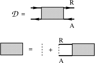
FIG. 4.: Diffuson diagrams. Cooperon diagrams differ from the ones for diffuson only in the direction of the arrow of the retarded Green function line.

The ensemble average of the pumped charge vanishes and the sign of $Q$ is random. To evaluate the typical value of this charge we consider the average $\langle Q_{A}Q_{B}\rangle$ for two different contours $A$ and $B$ on the parameter planes. To accomplish this task, we need to average the product of functions (22)

$${\cal I}={\Big{\langle}}{\cal F}(\epsilon_{1}+\epsilon,\mbox{\boldmath$X$}^{R},\mbox{\boldmath$X$}^{A}){\cal F}(\epsilon_{1},\mbox{\boldmath$Y$}^{R},\mbox{\boldmath$Y$}^{A}){\Big{\rangle}},$$ (45)

where function ${\cal F}$ is defined by Eq. (22).

Diagrammatic expression for ${\cal I}$ is shown on Fig. 5. Due to the relations (25), there is no need to renormalize the vertex $\Lambda$ by the dashed lines. For the same reason, vertices $\Lambda$ and $\Gamma$ can not appear in the same cell and, therefore, the Cooperon Eq. (37) does not contribute to ${\cal I}$ (45). We demonstrate in Sec. III, that this implies the difference in how the change of sign of magnetic field affects the pumped charge and the conductance [14, 15, 22].

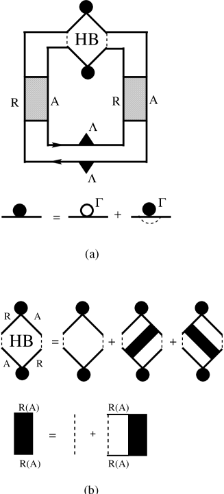
FIG. 5.: (a) Diagrammatic representation for the correlation function ${\cal I}$ from Eq. (45); (b) Hikami box.

The analytic expression for the diagram, Fig. 5, is

$${\cal I}=\frac{N_{l}N_{r}}{N_{ch}}{\cal B}{\cal D}\left(\epsilon;\mbox{\boldmath$X$}^{R}-\mbox{\boldmath$Y$}^{A}\right){\cal D}\left(-\epsilon;\mbox{\boldmath$Y$}^{R}-\mbox{\boldmath$X$}^{A}\right),$$ (46)

where diffuson propagator ${\cal D}$ is given by Eq. (38). The factor ${\cal B}$ in Eq. (46) is given by the set of diagrams Fig. 5b, which is analogous to the Hikami box for the disordered systems. It equals to

$${\cal B} = {\cal B}^{(1)}+{\cal B}^{(2)}+{\cal B}^{(3)};$$ (47)

$${\cal B}^{(1)} = \frac{\delta_{1}^{4}}{8\pi^{4}}\left[\left(\mbox{\boldmath$X$}^{R}-\mbox{\boldmath$X$}^{A}\right)\hat{C}_{0}\left(\mbox{\boldmath$Y$}^{A}-\mbox{\boldmath$Y$}^{R}\right)\right];$$ (48)

$${\cal B}^{(2)} = \frac{\delta_{1}^{2}}{4\pi^{2}{\cal D}\left(\epsilon;\mbox{\boldmath$X$}^{R}-\mbox{\boldmath$Y$}^{A}\right)};$$ (49)

$${\cal B}^{(3)} = \frac{\delta_{1}^{2}}{4\pi^{2}{\cal D}\left(-\epsilon;\mbox{\boldmath$Y$}^{R}-\mbox{\boldmath$X$}^{A}\right)}.$$ (50)

Substitution of the expression for ${\cal B}^{(2)}$ into Eq. (46) gives no contribution to ${\cal I}$ due to the relationship between ${\cal I}$ and $\Pi$, Eq. (22). Indeed, the part of ${\cal I}$ which depends on ${\cal B}^{(2)}$ does not contain $\mbox{\boldmath$X$}^{R}$. The contribution proportional to ${\cal B}^{(3)}$ vanishes in a similar way. Substituting ${\cal B}^{(1)}$ into Eq. (22), and the result into Eq. (46), we find

$${\Big{\langle}} \Pi \left(\epsilon_{1},\mbox{\boldmath$X$}+\mbox{\boldmath$Y$}\right)\Pi\left(\epsilon_{2},\mbox{\boldmath$Y$}\right){\Big{\rangle}}=\frac{8N_{l}N_{r}}{N_{ch}}\left[\hat{\varepsilon}\hat{C}_{0}\hat{\varepsilon}\right]_{ij}\frac{\partial^{2}}{\partial X_{i}\partial X_{j}}$$ (51)

$$\times \frac{1}{\left(\epsilon_{1}-\epsilon_{2}-\mbox{\boldmath$Z$}\cdot\mbox{\boldmath$X$}\right)^{2}+\left(N_{ch}+\mbox{\boldmath$X$}\hat{C}_{0}\mbox{\boldmath$X$}\right)^{2},}$$ (52)

Here we used the explicit form of the diffuson (38), introduced dimensionless energies (38) and took the spin degeneracy into account.

Now, we are in a state to evaluate the correlation function of charges pumped in a course of motion along contours $A$ and $B$ on the parameter plane. The result becomes compact if we choose new variables:

$$x = \frac{1}{\sqrt{N_{ch}}}\left(\hat{C}_{0}\right)^{1/2}\mbox{\boldmath$X$};$$ (54)

$$y = \frac{1}{\sqrt{N_{ch}}}\left(\hat{C}_{0}\right)^{1/2}\mbox{\boldmath$Y$};$$ (55)

$$z = \frac{1}{\sqrt{N_{ch}}}\left(\hat{C}_{0}\right)^{-1/2}\mbox{\boldmath$Z$}.$$ (56)

Let us discuss why $\mbox{\boldmath$x$},\mbox{\boldmath$y$},\mbox{\boldmath$z$}$ are natural dimensionless variables. Recall that we are dealing with open systems. Electronic escape time can be estimated as $\tau_{esc}\sim(N_{ch}\delta_{1})^{-1}$. All the energy levels have a finite width $\gamma\sim 1/\tau_{esc}\sim N_{ch}\delta_{1}>\delta_{1}$. It means that even at $T=0$ the pumping current is determined by the energy strip with a finite width $\gamma>\delta_{1}$. The number of the levels $n_{\gamma}$ in such a strip is a random function of the point in the parameter space. The correlation length $R=\left|\mbox{\boldmath$R$}\right|$ of this random function can be estimated from the equation

$$\mbox{\boldmath$R$}\mbox{\boldmath$Z$}+R_{i}\left[\hat{C}_{0}\right]_{ij}R_{j}\sim\gamma$$ (57)

The first term in the left hand side of Eq. (57) describes a homogeneous shift of the spectrum, while the second term represents random parametric oscillations [20]. Eq. (57) can be rewritten in terms of the new variables Eq. (5) as

$$\mbox{\boldmath$r$}\mbox{\boldmath$z$}+\mbox{\boldmath$r$}^{2}\sim 1$$ (58)

where $\mbox{\boldmath$r$}=(\hat{C}_{0}/N_{ch})^{1/2}\mbox{\boldmath$R$}$. As a result, $r\sim\mathrm{min}(1,\tilde{Z}^{-1})$. It means that in terms of the new variables $\mbox{\boldmath$x$},\mbox{\boldmath$y$},\mbox{\boldmath$z$}$ the pumping is weak (i.e. bilinear) provided that $r<\mathrm{min}(1,z^{-1})$. Finally,

$$\langle Q_{A}Q_{B}\rangle=-\frac{e^{2}N_{l}N_{r}}{N_{ch}^{2}}\int_{a}dx_{1}dx_{2}\int_{b}dy_{1}dy_{2}$$ (59)

$$\times\left(\frac{\partial}{\partial\mbox{\boldmath$x$}_{-}}\right)^{2}{\cal K}\left(\frac{2\pi T}{N_{ch}\delta_{1}},\mbox{\boldmath$z$}\cdot\mbox{\boldmath$x$}_{-},\mbox{\boldmath$x$}_{-}^{2}\right),$$ (60)

$$\mbox{\boldmath$x$}_{-}=\mbox{\boldmath$x$}-\mbox{\boldmath$y$},$$ (61)

where $\int_{a,b}$ denotes the integration within the area encompassed by contours $a$ and $b$, see Eq. (5), and dimensionless correlation function ${\cal K}$ is given by

$${\cal K}(u,v,w)=\frac{8}{\pi^{2}}\int_{-\infty}^{\infty}dh\frac{f(h)}{\left[\left(2uh+v\right)^{2}+\left(1+w\right)^{2}\right]}.$$ (62)

$$f(h)=\frac{(h\mathop{\mathrm{cotanh}}h-1)}{\left(\sinh h\right)^{2}}$$ (63)

Low temperature regime corresponds to $u\ll{\mathrm{m}ax}(1,v,w)$. In this limit

$${\cal K}(u,v,w)=\frac{8}{\pi^{2}}\frac{1}{v^{2}+\left(1+w\right)^{2}}.$$ (65)

while at high temperatures $u\gg{\mathrm{m}ax}(1,v,w)$

$${\cal K}(u,v,w)=\frac{4}{3\pi u}\left(\frac{1}{1+w}\right).$$ (66)

Therefore heating suppression of the mesoscopic fluctuations of $Q$ is similar to that of the conductance fluctuations.

Equations (59) – (62) are the main results of this section. They describe the correlation between the charge pumped due to the motion in the parameter space along the different contours at arbitrary temperature. Now, we are going to apply Eq. (59) to analyze the variance of the charge $\langle Q^{2}_{A}\rangle$.

C Weak Pumping.

If the characteristic magnitude of the potentials is so small that $\mbox{\boldmath$x$}_{-}^{2}\ll 1,\ \mbox{\boldmath$x$}_{-}\cdot\mbox{\boldmath$z$}\ll{\mathrm{m}ax}\left(1,T/(N_{ch}\delta_{1})\right)$, then the system is in bilinear response regime discussed in Refs. [10, 11]. In this case one can put $v=0,w=0$ in Eq. (62) after the differentiation. As a result

$$\langle Q_{A}^{2}\rangle=\frac{e^{2}N_{l}N_{r}S_{a}^{2}}{N_{ch}^{2}}\left[{\cal K}_{1}\left(\frac{2\pi T}{N_{ch}\delta_{1}}\right)+\mbox{\boldmath$z$}^{2}{\cal K}_{2}\left(\frac{2\pi T}{N_{ch}\delta_{1}}\right)\right],$$ (67)

where $S_{a}$ is the area enclosed by the contour $a$, in the parameter space $\mbox{\boldmath$x$}=\left(x_{1},x_{2}\right)$. Functions ${\cal K}_{1,2}(x)$ can be expressed through $f(h)$ from Eq. (62) in the following way:

$${\cal K}_{1}(u) = \frac{32}{\pi^{2}}\int_{-\infty}^{\infty}dh\frac{f(h)}{\left[4u^{2}h^{2}+1\right]^{2}}$$ (69)

$$= \left\{\matrix{\frac{32}{\pi^{2}},&u\ll 1;\cr\frac{8}{3\pi u},&u\gg 1},\right.$$ (70)

and

$${\cal K}_{2}(u) = \frac{16}{\pi^{2}}\int_{-\infty}^{\infty}dh\frac{f(h)\left(1-12u^{2}h^{2}\right)}{\left[4u^{2}h^{2}+1\right]^{3}}$$ (71)

$$= \left\{\matrix{\frac{16}{\pi^{2}},&u\ll 1;\cr\frac{4}{15\pi u^{3}},&u\gg 1.}\right.$$ (72)

In terms of the original pumping strength $X$ Eq. (67) acquires the form

$$\langle Q_{A}^{2}\rangle = \frac{e^{2}N_{l}N_{r}S_{A}^{2}}{N_{ch}^{4}}\left(\mathrm{det}\left[\hat{C}_{0}\right]\right)^{2}\times$$ (74)

$$\left[{\cal K}_{1}\left(\frac{2\pi T}{N_{ch}\delta_{1}}\right)+\frac{1}{N_{ch}}Z_{i}\left[\hat{C}_{0}^{-1}\right]^{ij}Z_{j}{\cal K}_{2}\left(\frac{2\pi T}{N_{ch}\delta_{1}}\right)\right]$$

Note that the specifics of the system enter only through the vector $Z$ and the tensor $\hat{C_{0}}$ defined in Eq. (38). In high temperature regime ${\cal K}_{2}\ll{\cal K}_{1}$. It means that the simultaneous shift of all levels ( determined by $z$) is not relevant for pumping. On the other hand, at $T\to 0$, this simultaneous shift of all levels may be important.

D Strong Pumping.

Let us now turn to the discussion of the opposite limit, $\mbox{\boldmath$x$}_{-}^{2}\gg 1$, where pumping is strong. In this regime it is more convenient to transform Eq. (59) to the contour integrals. Using Stokes theorem, we find

$$\langle Q_{A}^{2}\rangle = \frac{e^{2}N_{l}N_{r}}{N_{ch}^{2}}\oint_{a}dx_{i}\oint_{a}dy_{i}{\cal K}\left(\frac{2\pi T}{N_{ch}\delta_{1}},\mbox{\boldmath$z$}\mbox{\boldmath$x$}_{-},\mbox{\boldmath$x$}_{-}^{2}\right),$$ (75)

$$\mbox{\boldmath$x$}_{-} = \mbox{\boldmath$x$}-\mbox{\boldmath$y$},$$ (76)

We notice from Eq. (62) that the kernel ${\cal K}$ decreases rapidly at $\mbox{\boldmath$x$}_{-}^{2}\gtrsim 1$. Since the characteristic scale of the field itself is large $\mbox{\boldmath$x$}^{2}\gg 1$, we can perform the integration over $\mbox{\boldmath$x$}_{-}$ locally along the direction of the contour $d\mbox{\boldmath$x$}$. It gives

$$\langle Q_{A}^{2}\rangle=\frac{e^{2}N_{l}N_{r}}{N_{ch}^{2}}\oint_{a}dx{\cal L}\left(\frac{2\pi T}{N_{ch}\delta_{1}},\frac{\mbox{\boldmath$z$}\times\mbox{\boldmath$x$}}{\left|\mbox{\boldmath$x$}\right|}\right).$$ (77)

The kernel ${\cal L}$ can be expressed in terms of ${\cal K}$ from Eq. (62) as

$${\cal L}\left(u,v\right)=\int_{-\infty}^{\infty}dw{\cal K}(u,vw,w^{2}).$$ (78)

If the averaged level velocity is small, $y\ll 1$, we find from Eqs. (62) and Eqs. (77)

$$\langle Q_{A}^{2}\rangle=e^{2}{\ell}_{a}\frac{N_{l}N_{r}}{N_{ch}^{2}}{\cal L}_{1}\left(\frac{2\pi T}{N_{ch}\delta_{1}}\right),$$ (79)

where ${\ell}_{a}$ is the length of the contour $a$. Function ${\cal L}_{1}$ in Eq. (79) is given by

$${\cal L}_{1}(u) = \frac{2^{5/2}}{\pi}\int\frac{dhf(h)}{\left[1+4u^{2}h^{2}+\left(1+4u^{2}h^{2}\right)^{3/2}\right]^{1/2}}$$ (80)

$$= \matrix{\frac{4}{\pi},&u\ll 1\cr\frac{4}{3u},&u\gg 1}$$ (81)

In terms of the original pumping strength $X$, the dimensionless length of the contour ${\ell}_{a}$ ( Eq. (79)) acquires the form

$${\ell}_{a}=\frac{1}{N_{ch}}\oint_{A}\sqrt{dX_{i}\hat{C}^{ij}_{0}dX_{j}}$$ (82)

It is important to emphasize that in the case of the strong perturbation, the pumped charge is determined by the length of the contour rather than by its area, and it is not sensitive to the contour shape (provided that the contour is smooth on the scale of the order of unity). It has to be contrasted with the naive expectation $\langle Q_{A}^{2}\rangle\propto S_{a}$, which follows from independent addition of areas.

If $z$ is not small, the value of the pumped charge depends not only on the length of the contour but also on its shape. At low temperatures, we obtain from Eqs. (77), (78), and (65)

$$\langle Q_{A}^{2}\rangle=\frac{8e^{2}N_{l}N_{r}}{\pi N_{ch}^{2}}\oint_{a}dx\frac{1}{\left[4+\mbox{\boldmath$z$}^{2}\sin^{2}\left(\widehat{\mbox{\boldmath$z$}\mbox{\boldmath$x$}}\right)\right]^{1/2}},$$ (83)

where $\widehat{\mbox{\boldmath$z$}\mbox{\boldmath$x$}}$ is an angle between the vectors $z$ and $x$. At high temperature, $\langle Q^{2}\rangle$ does not depend on on the shape of the contour and is determined by Eqs. (79) and (81).

III Magnetic field effects on adiabatic pumping.

This section is devoted to the effect of the magnetic field on the pumped charge. In subsection  III B, we present a general discussion of the symmetries with respect to the time inversion. We demonstrate that, unlike the conductance, the pumped charge does not possess such a symmetry. This general conclusion is illustrated in subsection  III B by the model calculation of the second moment of the charge pumped through the quantum dot.

A Symmetry with respect to the reversal of the magnetic field

Let us now consider the pumping through the mesoscopic sample subjected to a magnetic field $B$. The general formalism of Sec. II A remains valid. One can infer from Eqs. (1) that the sign of the pumped charge changes together with the direction of the contour in the parameter space

$$Q_{\hookrightarrow}(B)=-Q_{\hookleftarrow}(B)$$ (84)

where ${\hookrightarrow}({\hookleftarrow})$ denote opposite direction of motion in the parameter space along the same contour. Indeed, curvature (6), is a single valued function of its parameters $X_{1},\ X_{2}$. Therefore, the only effect of reversal of the contour direction is to change the sign of the directed area $dX_{1}dX_{2}\to-dX_{1}dX_{2}$ without changing the integration domain. This immediately yields identity (84). Note that Eq. (84) relates the charges at the same magnetic field. It is also important to emphasize that Eq. (84) is valid for arbitrary strength of the pumping potential. It is not restricted by the bilinear response regime. Eq. (23) of Ref. [10]  $Q_{\hookrightarrow}(B)=-Q_{\hookleftarrow}(-B)$ together with Eq. (84) yield

$\displaystyle Q(B)=Q(-B),$

where the pumping is performed along the same contour in the parameter space. We intend to prove that, unlike for the two-terminal conductance[14, 15], such symmetry is not valid.

The exact (not-averaged) $S$ - matrix of the system changes with reversal of the magnetic field, $B$, as[23]:

$${\cal S}(E,B)=\left[{\cal S}(E,-B)\right]^{T}.$$ (85)

Symmetry relation for the two terminal conductance (1) follows directly from Eq. (85) [15]

$$G(-B)\propto{\mathrm{T}r}\left\{\hat{\tau}_{l}\hat{\cal S}(-B)\hat{\tau}_{r}\hat{\cal S}^{\dagger}(-B)\right\}=$$

$$={\mathrm{T}r}\left\{\hat{\tau}_{l}\hat{\cal S}^{T}(B)\hat{\tau}_{r}\hat{\cal S}^{*}(B)\right\}={\mathrm{T}r}\left\{\hat{\tau}_{r}\hat{\cal S}(B)\hat{\tau}_{l}\hat{\cal S}^{\dagger}(B)\right\}=$$

$$={\mathrm{T}r}\left\{\hat{\tau}_{l}\hat{\cal S}(B)\hat{\tau}_{r}\hat{\cal S}^{\dagger}(B)\right\}$$

We omitted factors independent of the magnetic field in the intermediate steps and used the unitarity of the $S$ - matrix. Therefore, the relation

$\displaystyle G(B)=G(-B)$

is exact.

Now let us turn to the pumped charge. Substituting Eq. (85) into Eq. (6), we find

$$\Pi\left(-B\right) = {\mathrm{I}m}\ {\mathrm{T}r}\left\{\hat{\tau}_{l}\frac{\partial\hat{\cal S}^{T}(B)}{\partial X_{2}}\frac{\partial\hat{\cal S}^{*}(B)}{\partial X_{1}}\right\}$$ (86)

$$= {\mathrm{I}m}\ {\mathrm{T}r}\left\{\hat{\tau}_{l}\frac{\partial\hat{\cal S}^{\dagger}(B)}{\partial X_{1}}\frac{\partial\hat{\cal S}(B)}{\partial X_{2}}\right\}=\Pi\left(B\right)$$ (87)

$$+ {\mathrm{I}m}\ {\mathrm{T}r}\left\{\hat{\tau}_{l}\left[\frac{\partial\hat{\cal S}^{\dagger}(B)}{\partial X_{1}};\frac{\partial\hat{\cal S}(B)}{\partial X_{2}}\right]\right\}$$ (88)

From Eq. (86) one obtains,

$$\Pi\left(B\right)-\Pi\left(-B\right)=\frac{i}{2}\varepsilon^{ij}{\mathrm{T}r}\left\{\hat{\tau}_{l}\left[\frac{\partial\hat{\cal S}^{\dagger}(B)}{\partial X_{i}};\frac{\partial\hat{\cal S}(B)}{\partial X_{j}}\right]\right\}.$$ (89)

Commutator in right-hand-side of Eq. (89) vanishes only if $S$-matrix is symmetric. This is not the case in the presence of a finite magnetic field. Therefore, there is no fundamental symmetry guarding the relation $\Pi\left(B\right)=\Pi\left(-B\right)$ as it was in the case for the two-terminal conductance, and the Eq. (23) of Ref. [10] does not hold. One can argue that it is the choice of the direction of the contour in the parameter space that violates the T - invariance and thus, $B\to-B$ symmetry.

The absence of the symmetry with respect to the reversal of the magnetic field, suggests that the correlation function $\langle Q(B_{1})Q(B_{2})\rangle$ depends on the difference $B_{1}-B_{2}$ only and vanishes at $|B_{1}-B_{2}|\to\infty$ (as it does in generic parametric statistics). Model calculation of the following subsection confirms this expectation.

B Model calculation of the second moment

In order to include the magnetic field into our description we have to lift the condition that matrix ${\cal H}_{mn}$ from Eqs. (12)–(13) is symmetric:

$\displaystyle{\cal H}_{mn}\to{\cal H}_{mn}+a{\cal H}_{mn}^{a},$

where ${\cal H}_{mn}^{a}$ is the random realization of antisymmetric $M\times M$ matrix and $a$ is the parameter proportional to the magnetic field. The resulting correlation function of two Hamiltonians at different values of the magnetic field $B_{1,2}$ can be conveniently presented in a form similar to Eq. (13) as

$$\langle{\cal H}_{nm}(B_{1}){\cal H}^{*}_{n^{\prime}m^{\prime}}(B_{2})\rangle=\left(\frac{\delta_{1}}{2\pi}\right)^{2}\times$$ (90)

$$\times\left[\delta_{nn^{\prime}}\delta_{mm^{\prime}}\left(4M-N_{h}^{D})+\delta_{mn^{\prime}}\delta_{nm^{\prime}}\left(4M-N_{h}^{C}\right)\right]\right.$$ (91)

Quantities $N_{h}^{D,C}$ characterize the effect of the magnetic field on the wave-functions of the closed dot and can be estimated as

$$N_{h}^{D}=g_{dot}\left(\frac{\Phi_{1}-\Phi_{2}}{\Phi_{0}}\right)^{2},\quad N_{h}^{C}=g_{dot}\left(\frac{\Phi_{1}+\Phi_{2}}{\Phi_{0}}\right)^{2}$$ (92)

where $g_{dot}\gg 1$ is the dimensionless conductance of the closed dot, $\Phi_{1(2)}$ is the magnetic flux through the dot which corresponds to the magnetic field $B_{1(2)}$, and $\Phi_{0}=hc/e$ is the flux quantum.

For the Green functions in Eq. (3) taken at different magnetic fields $B_{1},B_{2}$, the diffuson, Eq. (38), is modified as

$${\cal D}=\left(\frac{2\pi}{\delta_{1}}\right)^{2}\frac{1}{-i\epsilon+N_{ch}+N_{h}^{D}+i\mbox{\boldmath$Z$}\cdot\mbox{\boldmath$X$}+\mbox{\boldmath$X$}\hat{C}_{0}\mbox{\boldmath$X$}}$$ (93)

Diagrammatic representation, Fig. 5, and the expression for Hikami box (47) remain intact. Instead of Eq. (59) we obtain

$$\langle Q_{A}(B_{1})Q_{B}(B_{2})\rangle=-\frac{e^{2}N_{l}N_{r}}{N_{ch}^{2}}\int_{a}dx_{1}dx_{2}\int_{b}dy_{1}dy_{2}$$ (94)

$$\times\left(\frac{\partial}{\partial\mbox{\boldmath$x$}_{-}}\right)^{2}{\cal K}\left(\frac{2\pi T}{N_{ch}\delta_{1}},\mbox{\boldmath$z$}\cdot\mbox{\boldmath$x$}_{-},\mbox{\boldmath$x$}_{-}^{2}+\frac{N_{h}^{D}}{N_{ch}}\right),$$ (95)

$$\mbox{\boldmath$x$}_{-}=\mbox{\boldmath$x$}-\mbox{\boldmath$y$},$$ (96)

Here the variables $\mbox{\boldmath$x$},\mbox{\boldmath$y$},\mbox{\boldmath$z$}.$ are determined by Eq. (5) and the function ${\cal K}$ is given by Eq. (62).

Equation (96) is the main result of this section. It describes the sensitivity of the pumped charge to the magnetic field. One immediately realizes that the correlation function depends only on the difference of the magnetic fields in accord with the discussion in the previous subsection. Moreover the variance of the charge does not depend on the magnetic field (for bilinear response this result was obtained by Brouwer[11]). In terms of the diagrams, the absence of the symmetry with respect to the magnetic field reversal is revealed in the fact that the Cooperon does not contribute to the second moment even in the orthogonal case, $(B=0)$.

We conclude this section by the discussion of the asymptotics of the correlation function $\langle Q_{A}(B_{1})Q_{A}(B_{2})\rangle$ at finite magnetic field. We start with the weak pumping at low temperatures $T\ll\delta_{1}N_{ch}$. Instead of Eq. (67) one obtains

$$\langle Q_{A}(B_{1})Q_{A}(B_{2})\rangle=$$ (97)

$$=\frac{16e^{2}N_{l}N_{r}S_{a}^{2}}{\pi^{2}N_{ch}^{2}}\left[\frac{2N_{ch}^{3}}{\left(N_{ch}+N_{h}^{D}\right)^{3}}+\frac{N_{ch}^{4}\mbox{\boldmath$z$}^{2}}{\left(N_{ch}+N_{h}^{D}\right)^{4}}\right],$$ (98)

where $N_{h}^{D}$ is related to the magnetic fields by Eq. (92). If the dimensionless pumping potential is large (${\mathbf{x}}^{2}\gg\left(N_{h}^{D}/N_{ch}+1\right)$) and the average level velocity is small, $\mbox{\boldmath$Z$}=0$, we obtain instead of Eq. (79):

$$\langle Q_{A}^{2}\rangle=e^{2}{\ell}_{a}\left(\frac{4N_{l}N_{r}}{\pi N_{ch}^{2}}\right)\left(\frac{N_{ch}}{N_{ch}+N_{h}^{D}}\right)^{3/2}.$$ (99)

At high magnetic field, $\langle Q_{A}(B)Q_{A}(-B)\rangle$ rapidly decreases as $B^{-6}$, and one can use Eq. (97) for the bilinear response.

Finally, we discuss the variance of the pumped charge in the magnetic field in the limit of high temperatures ($T\gg{\mathrm{m}ax}(\frac{\delta_{1}(N_{ch}+N_{h}^{D})}{2\pi},{\mathbf{X}}^{2})$). For the weak pumping, assuming the average level velocity is small, we find

$$\langle Q_{A}^{2}\rangle=\left(\frac{4e^{2}N_{l}N_{r}S_{a}^{2}}{3\pi N_{ch}^{2}}\right)\left(\frac{N_{ch}\delta_{1}}{\pi T}\right)\left(\frac{N_{ch}}{N_{ch}+N_{h}^{D}}\right)^{2}.$$ (100)

In the strong pumping regime the high temperature asymptotic behavior instead of Eq. (79) is given by:

$$\langle Q_{A}^{2}\rangle=e^{2}{\ell}_{a}\left(\frac{2N_{l}N_{r}}{3N_{ch}^{2}}\right)\left(\frac{N_{ch}\delta_{1}}{\pi T}\right)\left(\frac{N_{ch}}{N_{ch}+N_{h}^{D}}\right)^{1/2}.$$ (101)

IV Discussion and conclusions

Our main results include dependence on the pumping strength, temperature and magnetic field.

Dependence of the pumping strength — At the small pumping potential, we essentially reproduced the results for bilinear response[11, 10], that $\langle Q^{2}\rangle\propto S_{A}^{2}$ with $S_{A}$ area being the area enclosed by the contour in the parametric space, see Eq. (67). This bilinear response regime, however, is valid only as long as the pumped charge is smaller than unity. The regime of strong pumping is analyzed for the first time in the present paper, see Eqs. (77) — (83). This regime is hallmarked by the dependence $\langle Q^{2}\rangle\propto\ell_{A}$, with $\ell_{A}$ being the length of the contour, which is substantially slower than naive expectation $\langle Q^{2}\rangle\propto S_{A}$. This slow dependence was already observed in Ref. [12]. We think that our conclusion about independence of the pumped charge variance on the shape of the contour deserves a careful check[24].

Temperature dependence — Our results for the high temperature regime $T\gtrsim N_{ch}\delta_{1}$ indicate that the variance of the charge $\langle Q^{2}\rangle$ is inversly proportional to the temperature $\langle Q^{2}\rangle\propto 1/T$. Experiment[12] demonstrates $\langle Q^{2}\rangle\propto 1/T^{2}$ in the high-temperature regime. This discrepancy was attributed to the presence of the temperature dependent dephasing, ignored in our treatment. In the simplistic models[25, 26], the dephasing is described by adding an extra factor $N_{\varphi}$ into the mass of diffuson and Cooperon (93). If such a questionable procedure is adopted, the effect of dephasing would be described by replacement $N^{D}_{h}\to N^{D}_{h}+N_{\varphi}$ in formulas of Sec. III B. We can see from Eqs. (100) — (101) that the same $N_{\varphi}$ produces different temperature dependences for the different regimes. Use of experimentally[26] known dependence $N_{\varphi}\propto T$, would produce the results $\langle Q^{2}\rangle\propto 1/T^{3}$ and $\langle Q^{2}\rangle\propto 1/T^{3/2}$ for weak and strong pumping respectively. We believe that the available experimental information is not sufficient yet for making detailed comparison with our theory.

Effect of the magnetic field — We have demonstrated in Sec. III A that there is no fundamental reason for the pumped current to be symmetric with respect to the magnetic field reversal, in a sharp contrast with the dependence of conductance on the magnetic field. The corresponding correlation functions were calculated in Sec. III B. It is demonstrated there that $\langle Q(B)Q(-B)\rangle\propto B^{-6}$ at large $B$. These conclusions contradict to Ref. [12] where the symmetry with respect to magnetic field reversal was reported. We can not explain this symmetry within the framework of our theory.

A

We demonstrate the equivalence between the equations  (1) and the approach of Ref. [10]. The demonstration will be based on equation of motion for the Green functions (18) related to the $S$ - matrices by Eq. (17). First, we substitute Eq. (17) into Eq. (20), and obtain

$$\Pi \left(E,\mbox{\boldmath$X$}\right)=2i\pi^{2}\nu^{2}\epsilon^{ij}\frac{\partial^{2}}{\partial X_{i}^{A}\partial X_{j}^{R}}$$ (A2)

$$\times{\mathrm{T}r}\left\{\hat{W}\hat{\tau}\hat{W}^{\dagger}\hat{G}^{R}\left(E,\mbox{\boldmath$X$}^{R}\right)\hat{W}\hat{W}^{\dagger}\hat{G}^{A}\left(E,\mbox{\boldmath$X$}^{A}\right)\right\}.$$

We will show now that matrix $\hat{G}^{R}\hat{W}\hat{W}^{\dagger}\hat{G}^{A}$ can be simplified significantly using the equations for the Green functions (18). We pre-multiply Eq. (18) for $\hat{G}^{A}$ by $\hat{G}^{R}$, we transpose Eq. (18) for $\hat{G}^{R}$ and post-multiply it by $\hat{G}^{A}$. Subtracting the results, we find

$$2i \pi\nu\hat{G}^{R}\left(E,\mbox{\boldmath$X$}^{R}\right)\hat{W}\hat{W}^{\dagger}\hat{G}^{A}\left(E,\mbox{\boldmath$X$}^{A}\right)$$ (A5)

$$=\hat{G}^{A}\left(E,\mbox{\boldmath$X$}^{A}\right)-\hat{G}^{R}\left(E,\mbox{\boldmath$X$}^{R}\right)$$

$$+\hat{G}^{R}\left(E,\mbox{\boldmath$X$}^{R}\right)\left[{\hat{H}}\left(\mbox{\boldmath$X$}^{R}\right)-{\hat{H}}\left(\mbox{\boldmath$X$}^{A}\right)\right]\hat{G}^{A}\left(E,\mbox{\boldmath$X$}^{A}\right).$$

Substituting Eq. (A5) into (A2), we obtain

$$\Pi\left(E,\mbox{\boldmath$X$}\right)=$$ (A6)

$$\epsilon^{ij}\frac{\partial}{\partial X_{i}}{\mathrm{T}r}\left\{\pi\nu\hat{W}\hat{\tau}\hat{W}^{\dagger}\hat{G}^{R}\left(E,\mbox{\boldmath$X$}\right)\frac{\partial\hat{H}\left(\mbox{\boldmath$X$}\right)}{\partial X_{j}}\hat{G}^{A}\left(E,\mbox{\boldmath$X$}\right)\right\}.$$ (A7)

If we recall that $\pi\nu\hat{W}\hat{\tau}\hat{W}^{\dagger}$ is an operator of the current from the dot through the left contact, we obtain Eq. (10) of Ref. [10], which proves that the physical mechanisms considered in Ref. [11] and [10] are identical.

REFERENCES

• [1] D.J. Thouless, Phys. Rev. B 27, 6083 (1983).
• [2] Q. Niu, Phys. Rev. Lett. 64, 1812 (1990).
• [3] D.V. Averin and K. K. Likharev, in Mesoscopic Phenomena in Solids, Eds. B.L. Altshuler, P.A. Lee and R.A. Webb (Elsevier, Amsterdam, 1991).
• [4] M.H. Devoret, D. Esteve and C. Urbina, in Les Houches. Session LXI Mesoscopic Quantum Physics Eds. E. Akkermans, G. Montambaux, J.-L. Pichard and J. Zin-Justin (Elsevier, Amsterdam, 1995).
• [5] L.P. Kouwenhoven et. al., in Proceedings of the Advanced Study Institute on Mesoscopic Electron Transport, Eds. L. Sohn, L.P. Kouwenhoven and G. Schoen (Kluwer, Series E, 1997).
• [6] L.P. Kouwenhoven et. al. Phys. Rev. Lett. 67, 1626 (1991).
• [7] I.L. Aleiner and A.V. Andreev, Phys. Rev. Lett. 81, 1286 (1998).
• [8] Effects of the Coulomb blockade on the conductance of the open dot were studied by P.W. Brouwer and I.L. Aleiner, Phys. Rev. Lett., 82, 390 (1999).
• [9] B. Spivak, F. Zhou, and M.T. Beal Monod, Phys. Rev. B, 51, 13226 (1995).
• [10] F. Zhou, B. Spivak, and B.L. Altshuler, Phys. Rev. Lett. 82, 608 (1999).
• [11] P.W. Brouwer, Phys. Rev. B 58, R10135 (1998).
• [12] M. Switkes, C.M. Marcus, K. Campman, and A.G. Gossard, Science, 283, 1907 (1999).
• [13] B.L. Altshuler and D.E. Khmelnitskii, JETP Letters, 42, 359 (1985).
• [14] L. Onsager, Phys. Rev. 38, 2265 (1931).
• [15] M. Büttiker, Phys. Rev. Lett. 57, 1761 (1986).
• [16] M. Büttiker, H. Thomas, and A. Pretre, Z. Phys. B 94, 133 (1994).
• [17] C.W.J. Beenakker, Rev. Mod. Phys, 69, 731, (1997).
• [18] A.A. Abrikosov, L.P. Gorkov, I.E. Dzyaloshinskii, Methods of Quantum Field Theory in Statistical Physics, (Prentice–Hall, Englewood Cliffs, NJ, 1963).
• [19] B.L. Altshuler and A.G. Aronov, in Electron-Electron Interactions in Disordered Systems, A.L.Efros and M.Pollak eds., (North-Holland, Amsterdam, 1985)
• [20] B.D. Simons and B.L. Altshuler, Phys. Rev. Lett., 70, 4063, (1993).
• [21] B.L. Altshuler and B.I. Shklovskii, Sov. Phys. JETP 64, 127, (1986)
• [22] B.L.Altshuler and B.Z.Spivak, JETP Lett. 42, 447 (1985).
• [23] L.D. Landau and E.M. Lifshitz, Quanutm mechanics, 3rd edition, (Pergamon Press, 1977).
• [24] Detailed comparison with the data was performed recently by M. Vavilov (private communication).
• [25] H.U. Baranger, P.A. Mello, Phys. Rev. B, 51, 4703, (1995); P.W. Brouwer and C.W.J. Beenakker, ibid., 51, 7739, (1995); ibid., 55, 4695, (1997); I.L. Aleiner and A.I. Larkin. ibid., 54, 14423 (1996); E. McCann and I.V. Lerner, ibid., 57, 7219 (1998).
• [26] A.G. Huibers et. al., Phys. Rev. Lett., 81, 200 (1998).