Evaporative Cooling of a Two-Component Degenerate Fermi Gas

Abstract

We derive a quantum theory of evaporative cooling for a degenerate Fermi gas with two constituents and show that the optimum cooling trajectory is influenced significantly by the quantum statistics of the particles. The cooling efficiency is reduced at low temperatures due to Pauli blocking of available final states in each binary collision event. We compare the theoretical optimum trajectory with experimental data on cooling a quantum degenerate cloud of potassium-40, and show that temperatures as low as 0.3 times the Fermi temperature can now be achieved.

PACS: 03.75.Fi, 05.30 Fk, 05.20.Dd, 67.40.Fd

The recent demonstrations of Bose-Einstein condensation in dilute alkali and hydrogen gases have required the ability to reach extremely low temperatures in the micro-Kelvin to nano-Kelvin scale. To date, this has been possible only by using the experimental technique of forced evaporative cooling [2]. Efficient evaporative cooling can allow the temperature of a gas to be reduced by orders of magnitude without prohibitive loss in the number of atoms. It has universal application to cool magnetically trapped atomic and molecular vapors and has already been applied to produce quantum degenerate clouds of rubidium [3], sodium [4], lithium [5], potassium [6], and hydrogen [7].

For a bosonic gas, cooling can be continued to the point where no discernible normal component of the gas is present, closely approximating a zero temperature system. Demonstrating the ability to reach this regime has been a prerequisite to many of the recent experiments on collective effects in these systems. Collective phenomena that have now been observed include linear response [8, 9, 10, 11], surface modes [12], and topological excitations such as vortices [13, 14]. A current goal is to observe the conjugate low-temperature phenomena in a fermionic gas when it is cooled well below the onset of quantum degeneracy [15, 16, 17, 18].

In evaporative cooling, a “cut” is made at a prescribed energy and all atoms with energies greater than the cut are removed from the system. The remaining atoms will rethermalize by collisions to form an equilibrium with a lower temperature. The crucial parameter that determines the timescale for cooling is therefore the rate of rethermalization $\Gamma$. For a dilute gas at temperatures where quantum statistics do not play a role, rethermalization is determined by the elastic collision rate, given by $\Gamma=\bar{n}\sigma v$, where $\bar{n}$ is the spatially averaged density-weighted density, $\sigma$ is the collision cross section, and $v$ is the root-mean-square velocity of the colliding species. In a harmonic trap, $\Gamma$ may increase as the gas is cooled despite the obvious reduction in average velocity. The reason for this is simply that as the cloud cools, the atoms fall to the bottom of the trap and become more tightly confined, increasing the number density $n$ and more than compensating for the loss in energy per particle. Achieving this regime, known as runaway evaporation, is typically an experimental prerequisite for following a cooling trajectory that leads to a quantum degenerate gas.

For bosons, once the temperature is reduced below the critical temperature for Bose-Einstein condensation to occur, effects due to quantum statistics assist the evaporation. Consider a typical collision event involving two atoms from the normal thermal gas that initially have approximately the mean energy of the distribution. The presence of a Bose-Einstein condensate modifies the scattering probability into each possible final state and enhances the likelihood of stimulated scattering of one of the atoms into the condensate. The other atom then obtains the total energy of the initial pair and can be removed by the evaporative cut. Clearly this type of collision leads to very efficient evaporative cooling.

The opposite situation is true for fermions. As the temperature falls below the Fermi temperature, efficient collisions turn off due to Pauli blocking since the states of lowest energy become occupied with high probability [19]. In this paper we study this effect on the achievable optimum evaporation trajectory. Our calculations are motivated by the first application of evaporative cooling to produce a quantum degenerate Fermi gas [6]. This recent experiment has opened the door to the study of Fermi statistics in an extremely dilute regime—perhaps eventually allowing for the possibility of investigating Cooper pairing and the BCS phase transition in these dilute systems.

At typical temperatures of interest, collisions between atom pairs are purely $s$-wave since the characteristic collision energies are well below the centrifugal barrier associated with channels of non-zero orbital angular momenta [20]. Since for fermions the total wavefunction must be antisymmetric with respect to exchange of any pair of atoms, $s$-wave collisions are only possible if at least two internal atomic hyperfine states are simultaneously present, or alternatively if sympathetic cooling is performed with a distinguishable species, such as a different isotope or a different element [21, 22]. Here, we consider the first of these possibilities—a two-component Fermi gas.

The Hamiltonian for this system may be separated into two parts, ${H}={H}_{0}+{H}_{1}$ where ${H}_{0}$ is the usual single particle energy of the system and ${H}_{1}$ describes binary collisions. The Hamiltonian ${H}_{0}$ for a two-component mixture confined in a three-dimensional harmonic oscillator is

$${H}_{0}=\sum_{\mbox{\boldmath$\scriptstyle n$}}E_{\mbox{\boldmath$\scriptstyle n$}}\left(a^{{\dagger}}_{\mbox{\boldmath$\scriptstyle n$}}a^{\phantom{{\dagger}}}_{\mbox{\boldmath$\scriptstyle n$}}+b^{{\dagger}}_{\mbox{\boldmath$\scriptstyle n$}}b^{\phantom{{\dagger}}}_{\mbox{\boldmath$\scriptstyle n$}}\right),$$ (1)

where we have assumed the potential is identical for both species. The summation is taken over the three integer components of $\mbox{\boldmath$n$}=(n_{x},n_{y},n_{z})$. If the harmonic potential is isotropic with oscillation frequency $\omega$ then $E_{\mbox{\boldmath$\scriptstyle n$}}=\hbar\omega(n_{x}+n_{y}+n_{z}+3/2)$. The annihilation operators for the two components, $a_{\mbox{\boldmath$\scriptstyle n$}}$ and $b_{\mbox{\boldmath$\scriptstyle n$}}$, obey the usual Fermi commutation relations. Binary collisions are described by the interaction Hamiltonian

$$\hat{H}_{1}=\sum_{\mbox{\boldmath$\scriptstyle n$},\mbox{\boldmath$\scriptstyle m$},\mbox{\boldmath$\scriptstyle q$},\mbox{\boldmath$\scriptstyle p$}}C_{\mbox{\boldmath$\scriptstyle n$},\mbox{\boldmath$\scriptstyle m$};\mbox{\boldmath$\scriptstyle q$},\mbox{\boldmath$\scriptstyle p$}}\,\,a^{{\dagger}}_{\mbox{\boldmath$\scriptstyle n$}}b^{{\dagger}}_{\mbox{\boldmath$\scriptstyle m$}}b^{\phantom{{\dagger}}}_{\mbox{\boldmath$\scriptstyle q$}}a^{\phantom{{\dagger}}}_{\mbox{\boldmath$\scriptstyle p$}},$$ (2)

where the matrix element is

$$C_{\mbox{\boldmath$\scriptstyle n$},\mbox{\boldmath$\scriptstyle m$};\mbox{\boldmath$\scriptstyle q$},\mbox{\boldmath$\scriptstyle p$}}=U_{0}\int d^{3}x\,{\alpha}^{*}_{\mbox{\boldmath$\scriptstyle n$}}(\mbox{\boldmath$x$}){\beta}^{*}_{\mbox{\boldmath$\scriptstyle m$}}(\mbox{\boldmath$x$}){\beta}^{\phantom{*}}_{\mbox{\boldmath$\scriptstyle q$}}(\mbox{\boldmath$x$}){\alpha}^{\phantom{*}}_{\mbox{\boldmath$\scriptstyle p$}}(\mbox{\boldmath$x$}).$$ (3)

The oscillator eigenfunctions ${\alpha}_{\mbox{\boldmath$\scriptstyle n$}}$ and ${\beta}_{\mbox{\boldmath$\scriptstyle n$}}$ form a complete orthonormal basis that spans the two-component Hilbert space. In calculating the matrix element, we have replaced the physical two-particle potential by a contact potential. The dimensional prefactor is $U_{0}=4\pi\hbar^{2}a/m$, where $m$ is the atomic mass, and $a$ is the $s$-wave scattering length, which includes contributions from both direct and exchange scattering.

Although, in principle, one could solve the evolution of this isolated many-body system, we are primarily interested here in a simplified description on a coarse-grained timescale. Such a description is given by quantum kinetic theory where a set of relevant observables are quantities of interest. The underlying theoretical framework derives from the property that collisions in the dilute gas are extremely well separated in time. This allows the Born and Markov approximations to be made and the subsequent derivation of a perturbative theory in lowest orders of the interaction Hamiltonian [23]. The relevant observables are the populations of the two species (diagonal elements of the single particle density matrix): $A_{\mbox{\boldmath$\scriptstyle n$}}=\langle a^{{\dagger}}_{\mbox{\boldmath$\scriptstyle n$}}a^{\phantom{{\dagger}}}_{\mbox{\boldmath$\scriptstyle n$}}\rangle$ and $B_{\mbox{\boldmath$\scriptstyle n$}}=\langle b^{{\dagger}}_{\mbox{\boldmath$\scriptstyle n$}}b^{\phantom{{\dagger}}}_{\mbox{\boldmath$\scriptstyle n$}}\rangle$.

This approach must be extended in order to treat boson-fermion mixtures, or Fermi gases at temperatures where Cooper pairing is important. In those situations it would be necessary to expand the set of relevant observables to consider diagonal and off-diagonal contributions to the normal and anomalous densities, as well as the role of mean-fields [24].

Following this procedure, the quantum kinetic equations (also referred to as the “Quantum Boltzmann Equations”) for the two-component Fermi gas are given by

$${dA_{\mbox{\boldmath$\scriptstyle n$}}\over dt} = {1\over 2}\sum_{\mbox{\boldmath$\scriptstyle m$},\mbox{\boldmath$\scriptstyle q$},\mbox{\boldmath$\scriptstyle p$}}W_{\mbox{\boldmath$\scriptstyle n$},\mbox{\boldmath$\scriptstyle m$};\mbox{\boldmath$\scriptstyle q$},\mbox{\boldmath$\scriptstyle p$}}\,\Bigl{\{}A_{\mbox{\boldmath$\scriptstyle p$}}B_{\mbox{\boldmath$\scriptstyle q$}}(1-B_{\mbox{\boldmath$\scriptstyle m$}})(1-A_{\mbox{\boldmath$\scriptstyle n$}})$$ (5)

$$\quad{}-A_{\mbox{\boldmath$\scriptstyle n$}}B_{\mbox{\boldmath$\scriptstyle m$}}(1-B_{\mbox{\boldmath$\scriptstyle q$}})(1-A_{\mbox{\boldmath$\scriptstyle p$}})\Bigr{\}},$$

$${dB_{\mbox{\boldmath$\scriptstyle m$}}\over dt} = {1\over 2}\sum_{\mbox{\boldmath$\scriptstyle n$},\mbox{\boldmath$\scriptstyle q$},\mbox{\boldmath$\scriptstyle p$}}W_{\mbox{\boldmath$\scriptstyle n$},\mbox{\boldmath$\scriptstyle m$};\mbox{\boldmath$\scriptstyle q$},\mbox{\boldmath$\scriptstyle p$}}\,\Bigl{\{}A_{\mbox{\boldmath$\scriptstyle p$}}B_{\mbox{\boldmath$\scriptstyle q$}}(1-B_{\mbox{\boldmath$\scriptstyle m$}})(1-A_{\mbox{\boldmath$\scriptstyle n$}})$$ (7)

$$\quad{}-A_{\mbox{\boldmath$\scriptstyle n$}}B_{\mbox{\boldmath$\scriptstyle m$}}(1-B_{\mbox{\boldmath$\scriptstyle q$}})(1-A_{\mbox{\boldmath$\scriptstyle p$}})\Bigr{\}},$$

where the transition rates are found from Fermi’s golden rule

$$W_{\mbox{\boldmath$\scriptstyle n$},\mbox{\boldmath$\scriptstyle m$};\mbox{\boldmath$\scriptstyle q$},\mbox{\boldmath$\scriptstyle p$}}={2\pi\over\hbar}|C_{\mbox{\boldmath$\scriptstyle n$},\mbox{\boldmath$\scriptstyle m$};\mbox{\boldmath$\scriptstyle q$},\mbox{\boldmath$\scriptstyle p$}}|^{2}{\delta_{E_{\mbox{\boldmath$\scriptscriptstyle m$}}+E_{\mbox{\boldmath$\scriptscriptstyle n$}},E_{\mbox{\boldmath$\scriptscriptstyle q$}}+E_{\mbox{\boldmath$\scriptscriptstyle p$}}}\over\hbar\omega}.$$ (8)

Note the factors such as $(1-A_{\mbox{\boldmath$\scriptstyle n$}})$ and $(1-B_{\mbox{\boldmath$\scriptstyle m$}})$ give rise to the mechanism known as Pauli blocking. The Kronecker delta function, $\delta$, constrains the collision to be precisely on the energy shell. This is an unphysical artifact of the Markov approximation that is valid for the dilute gas only when the elastic collision rate is much less than the oscillation frequency in the trap. Otherwise the collisional broadening of the levels would be greater than their spacing, and the energy basis we use here would not be an appropriate choice since off-diagonal elements would then be important. We assume ergodicity by assigning equal population to each state in the degenerate manifold of states with the same principal quantum number $n$ (and therefore the same energy). We denote the ergodic populations by $A_{e_{n}}$ and $B_{e_{n}}$ (indexed only by the discrete values of the energy $e_{n}$) which are related to previously defined populations for an arbitrary quantum state $A_{\mbox{\boldmath$\scriptstyle n$}}$ and $B_{\mbox{\boldmath$\scriptstyle n$}}$ by

$$g_{e_{n}}A_{e_{n}} = \sum_{\mbox{\boldmath$\scriptstyle n$}}\delta_{e_{n},E_{\mbox{\boldmath$\scriptscriptstyle n$}}}A_{\mbox{\boldmath$\scriptstyle n$}},$$ (9)

$$g_{e_{n}}B_{e_{n}} = \sum_{\mbox{\boldmath$\scriptstyle n$}}\delta_{e_{n},E_{\mbox{\boldmath$\scriptscriptstyle n$}}}B_{\mbox{\boldmath$\scriptstyle n$}},$$ (10)

with $g_{e_{n}}$ denoting the degeneracy of states for the three-dimensional harmonic oscillator

$$g_{e_{n}}={1\over 2}(n+1)(n+2).$$ (11)

The quantum kinetic equations given in Eq. (7) may be simplified by approximating the summations by integrals over continuous distributions. This is typically always a good approximation for fermions, since for a sufficiently large sample, a macroscopic number of states are occupied even at very low temperature. The quantum kinetic equations then describe the rate of transfer of population between continuous distribution functions. We denote these functions (of a continuous energy variable $e$) as $A(e)$ and $B(e)$, which evolve according to

$$\rho(e_{n}){dA(e_{n})\over dt} = {m\sigma\over\pi^{2}\hbar^{3}}\int de_{m}de_{q}de_{p}\,\delta(\Delta)\rho(e_{\rm min})$$ (14)

$$\Bigl{\{}A(e_{p})B(e_{q})[1-B(e_{m})][1-A(e_{n})]$$

$$-A(e_{n})B(e_{m})[1-B(e_{q})][1-A(e_{p})]\Bigr{\}}$$

$$\rho(e_{m}){dB(e_{m})\over dt} = {m\sigma\over\pi^{2}\hbar^{3}}\int de_{n}de_{q}de_{p}\,\delta(\Delta)\rho(e_{\rm min})$$ (17)

$$\Bigl{\{}A(e_{p})B(e_{q})[1-B(e_{m})][1-A(e_{n})]$$

$$-A(e_{n})B(e_{m})[1-B(e_{q})][1-A(e_{p})]\Bigr{\}},$$

where $e_{\rm min}=\min\{e_{n},e_{m},e_{p},e_{q}\}$ and $\Delta=e_{n}+e_{m}-e_{q}-e_{p}$. The quantum mechanical cross-section applicable here is $\sigma=4\pi a^{2}$ since the products of a collision event are in quantum mechanically distinguishable spin states [25]. The density of states $\rho(e)$ for the three-dimensional harmonic oscillator can be found from the large $n$ limit of Eq. (11), which gives $\rho(e)={1\over 2}e^{2}$. Although these equations are similar in form to the discrete version in Eq. (7), a key simplification has been the replacement of the collision kernel [defined in Eq. (8)] by $\rho(e_{\rm min})$; which is the classical limit [26]. As was shown in Ref. [27], the convergence to the classical limit is very rapid as $e_{\rm min}$ is raised. Significant quantum correction occurs only when both of the colliding atoms are in the lowest few (of order one to five) states of the harmonic oscillator. These lowest energy collisions give a microscopic correction to the collision rate when the particles have Fermi statistics and are typically distributed over a macroscopic number of levels of the oscillator. The situation is quite different for the quantum degenerate Bose gas where a careful treatment of these low energy collisions is usually crucial due to the possibility of condensate mean-fields.

While the simultaneous equations in Eq. (17) may be solved by direct numerical integration, the calculation is cumbersome given the multidimensional integrals that must be performed at each timestep. We provide a more intuitive approach that is motivated by the near equilibrium distributions expected when the elastic collision rate is sufficiently high. We assume that the form of the population distribution functions for both components are given by a truncated Fermi-Dirac distribution $F(e)$ as defined by

$$F(e)=\left\{\begin{array}[]{cc}(\exp[{\beta(e-\mu)}]+1)^{-1}&e<K\\ 0&{\rm otherwise}\end{array}\right..$$ (18)

A similar method was introduced in Ref. [26] to treat the evaporative cooling of a classical gas. For simplicity, we also take the simplest case of $A(e)=B(e)=F(e)$ at all times, since if the distributions of the two components are initially identical they will remain so due to the symmetry of the equations. This means that the distribution functions for both species are parameterized by the same three variables: (i) an inverse temperature $\beta$, (ii) a chemical potential $\mu$, and (iii) a cut energy $K$. Given a value for the cut energy, $\beta$ and $\mu$ can be solved to give simultaneously the correct total number of atoms in one component $N$, and total energy of these atoms $E$, according to

$$\int_{0}^{K}de\,\rho(e)F(e)=N,$$ (19)

$$\int_{0}^{K}de\,e\rho(e)F(e)=E.$$ (20)

The truncated Fermi-Dirac distribution function is illustrated in Fig. 1 for the initial conditions of the evaporative simulation.

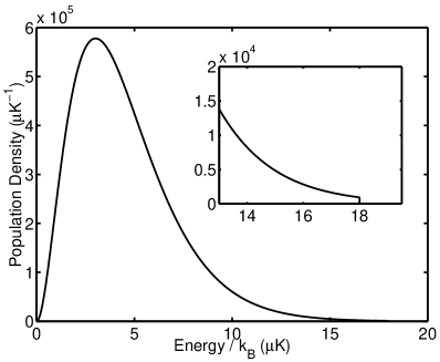
FIG. 1.: The truncated Fermi-Dirac distribution. The graph shows the distribution function, $\rho(e)F(e)$, as a function of $e/k_{B}$ where $k_{B}$ is Boltzmann’s constant. The parameters used were those for the start of the evaporation simulation with $N=3.2\times 10^{6}$, $E=3Nk_{B}T$ where $T=1.5\,\mu$K, and $K=4E/N$. The inset shows a magnified view of the discontinuity at the cut energy.

The simulation algorithm is the following:

1. Starting with given $N$, $E$, and $K$, solve Eq. (20) to find $\beta$ and $\mu$.

2. Consider propagation of the kinetic equations for a time step $dt$ and determine the change in number $dN_{1}$ and energy $dE_{1}$ due to atoms colliding and gaining energy above the cut $K$,

   $$dN_{1} = dt{m\sigma\over\pi^{2}\hbar^{3}}\int_{K}^{2K}de_{n}\int_{0}^{2K-e_{n}}de_{m}\int_{e_{m}+e_{n}-K}^{K}de_{p}$$ (22)

   $$\rho(e_{m})F(e_{m}+e_{n}-e_{p})F(e_{p})[1-F(e_{m})]$$

   $$dE_{1} = dt{m\sigma\over\pi^{2}\hbar^{3}}\int_{K}^{2K}de_{n}\int_{0}^{2K-e_{n}}de_{m}\int_{e_{m}+e_{n}-K}^{K}de_{p}$$ (24)

   $$e_{n}\rho(e_{m})F(e_{m}+e_{n}-e_{p})F(e_{p})[1-F(e_{m})]$$

3. Simulate background loss (energy-independent removal of atoms arising from non-ideal vacuum conditions in experiments) with rate $\gamma$ from the trap

   $$dN_{2} = \gamma Ndt,$$ (25)

   $$dE_{2} = \gamma Edt.$$ (26)

4. Lower the cut energy, from $K$ to a new value $K^{\prime}$ and find the change in number and energy due to trimming the highest energy atoms:

   $$dN_{3} = \int_{K^{\prime}}^{K}de\,\rho(e)F(e),$$ (27)

   $$dE_{3} = \int_{K^{\prime}}^{K}de\,e\rho(e)F(e).$$ (28)

5. Update the number and energy

   $$N \rightarrow N-\sum_{\sigma}dN_{\sigma},$$ (29)

   $$E \rightarrow E-\sum_{\sigma}dE_{\sigma},$$ (30)

   and repeat this sequence starting again from step 1.

A technical point is that solving Eq. (20) for $\beta$ and $\mu$ is a two-dimensional root finding problem that can potentially be non-trivial. We use a multidimensional Newton-Raphson algorithm that will rapidly produce a good estimate of the value of the solutions in a few iterations. To find a good estimate to start with, we employ a simple three-point polynomial extrapolation of solutions from previous timesteps. In this extrapolation we use the cut energy $K$ as the independent variable, rather than the step number or time.

Although this method may be used to calculate the evaporation trajectory for an arbitrary time dependence of the cut energy, we are most interested here in determining the optimum path. During the evaporation simulation, we follow a trajectory that maximizes the energy removed per particle from the system. That is, we choose a value for $K^{\prime}$ in such a way as to numerically maximize

$${\sum_{\sigma}dE_{\sigma}\over\sum_{\sigma}dN_{\sigma}}$$ (31)

for the subsequent timestep.

In Fig. 2, we show the calculated optimum evaporation trajectory for the two-component Fermi gas. In order to indicate the level of quantum degeneracy, we have normalized energies and temperatures by dividing them by the Fermi energy and Fermi temperature (see caption). The optimum cut energy approaches closely the Fermi surface towards the end of the simulation. While the ideal evaporative trajectory demonstrates the theoretical possibility for achieving very low temperatures—with the chemical potential tending towards the Fermi energy and with a macroscopic population remaining—the efficiency of the evaporation trajectory falls dramatically as the system becomes degenerate.

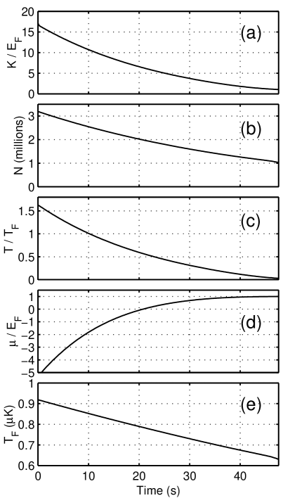
FIG. 2.: Optimum evaporation trajectory. The parameters used were those typical for the experiment reported in Ref. [6]; $\omega/2\pi=70$ Hz is the geometric mean of the trap frequencies, $m$ is the mass of potassium-40, $\gamma=1/350$ Hz, and the scattering is dominated by the triplet channel with $a=157a_{0}$ where $a_{0}$ is the Bohr radius [20]. The initial conditions used are given in Fig. 1. (a) The optimized cut energy $K$ divided by the Fermi energy $E_{F}$. For a three-dimensional harmonic oscillator the Fermi energy is $E_{F}=(6N)^{1/3}\hbar\omega$. (b) The number of atoms in each component. (c) The temperature $T$, defined for the truncated Fermi-Dirac distribution as $T=1/(\beta k_{B})$. The temperature is normalized by the Fermi temperature $T_{F}=E_{F}/k_{B}$. (d) The chemical potential $\mu$ in units of $E_{F}$. (e) The Fermi temperature $T_{F}$.

This is shown by the elastic collision rate $\Gamma$ defined by

$$\Gamma = {m\sigma\over 2N\pi^{2}\hbar^{3}}\int de_{n}de_{m}de_{p}de_{q}\,\delta(\Delta)\rho(e_{\rm min})$$ (33)

$$\quad F(e_{p})F(e_{q})[1-F(e_{m})][1-F(e_{n})],$$

which is illustrated in Fig. 3. As the chemical potential becomes positive, and Pauli blocking of available final states begins to play an important role, the elastic collision rate falls sharply. Since the elastic collision rate determines the timescale for rethermalization, at the end of the simulation, evaporative cooling has virtually ceased. As this figure dramatically illustrates, towards the end of the evaporation trajectory, the elastic collision rate may be more than an order of magnitude suppressed from the value it would have if Pauli blocking of final states was absent.

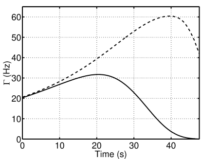
FIG. 3.: Elastic collision rate per atom for the optimized evaporation trajectory. The solid line shows the true collision rate as defined in Eq. (33). The dashed line shows what the collision rate would be in the absence of Pauli blocking, by artificially replacing the $[1-F(e_{m})][1-F(e_{n})]$ factors in Eq. (33) by unity.

In Fig. 4, we illustrate this trajectory on a semilog graph of temperature versus number and compare with experimental data. The data are taken by evaporating a two-component gas of ⁴⁰K as described in Ref. [6]. For the portion of the evaporation trajectory shown in Fig. 4 evaporation occurs using a 50/50 mixture of two spin states confined in a cylindrically symmetric harmonic trap whose radial frequency is 137 Hz and axial frequency is 19.5 Hz. After evaporation, one of the spin components is removed quickly (within 0.3 s) with the application of a frequency-swept microwave field; this removal provides a small amount of additional evaporative cooling that reduces the cloud temperature by 20%. The comparison shown in Fig. 4 illustrates that although it is possible theoretically to reach very low temperatures, the data corresponds to less efficient evaporative cooling and is presumably limited by experimental artifacts. These experimental limitations could include heating of the trapped gas, finite energy resolution of the evaporative cut, reduced dimensionality of the evaporative cut, and other similar problems.

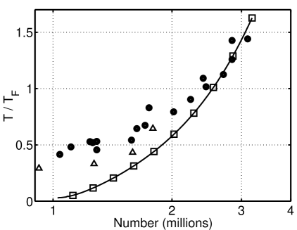
FIG. 4.: Optimum evaporation trajectory. The $\Box$ symbols show points on the theoretical evaporation trajectory at time intervals of 5 s. For comparison, the $\bullet$ symbols show experimental data points giving a typical evaporation trajectory. The $\triangle$ symbols show the lowest $T/T_{F}$ achieved in our current experiment, as described in the text.

In the current experiment we have recently found that improving the stability of the magnetic trapping field increased the highest achievable quantum degeneracy from $T/T_{F}=0.5$ to $T/T_{F}=0.3$. The low temperature part of an experimental exaporation trajectory that reached $T/T_{F}=0.3$ is also shown in Fig. 4. For this data we used a much slower removal of the second spin component (within 25 s) to provide additional evaporative cooling which is not included in the theory. The experimental progress suggests that further technical improvements may enable experiments to approach the low $T/T_{F}$ values that appear possible theoretically. Furthermore Fig. 3 shows that the dramatic suppression of the elastic collision rate due to Pauli blocking could be observed at the lowest temperatures of current experiments.

We would like to thank J. Cooper, R. Walser, B. Anderson, and J. Bohn for discussions. M. Holland acknowledges support for this work from the Department of Energy. D. Jin and B. DeMarco acknowledge funding from the Office of Naval Research and the National Science Foundation.

REFERENCES

- [1]
- [2] H. F. Hess, Phys. Rev. B 34 3476 (1986).
- [3] M. H. Anderson, J. R. Ensher, M. R. Matthews, C. E. Wieman, and E. A. Cornell, Science 269, 198 (1995).
- [4] K. B. Davis, M.-O. Mewes, M. R. Andrews, N. J. van Druten, D. S. Durfee, D. M. Kurn, and W. Ketterle, Phys. Rev. Lett. 75, 3969 (1995).
- [5] C. C. Bradley, C. A. Sackett, J. J. Tollet, and R. G. Hulet, Phys. Rev. Lett. 75, 1687 (1995); Erratum. ibid. 79, 1170 (1997).
- [6] B. DeMarco and D. S. Jin, Science 285, 1703 (1999).
- [7] D. G. Fried, T. C. Killian, L. Willmann, D. Landhuis, S. C. Moss, D. Kleppner, T. J. Greytak, Phys. Rev. Lett. 81 3811 (1998).
- [8] D. S. Jin, J. R. Ensher, M. R. Matthews, C. E. Wieman, E. A. Cornell, Phys. Rev. Lett. 77, 420 (1996).
- [9] D. S. Jin, M. R. Matthews, J. R. Ensher, C. E. Wieman, E. A. Cornell, Phys. Rev. Lett. 78, 764 (1997).
- [10] M.-O. Mewes, M. R. Andrews, N. J. vanDruten, D. M. Kurn, D. S. Durfee, C. G. Townsend, W. Ketterle, Phys. Rev. Lett. 77, 988 (1996).
- [11] D. M. Stamper-Kurn, H. J. Miesner, S. Inouye, M. R. Andrews, W. Ketterle, Phys. Rev. Lett. 81, 500 (1998).
- [12] R. Onofrio, D. S. Durfee, C. Raman, M. Kohl, C. E. Kuklewicz, W. Ketterle, cond-mat/9908340.
- [13] J. E. Williams and M. J. Holland, Nature 401, 569 (1999).
- [14] M. R. Matthews, B. P. Anderson, P. C. Haljan, D. S. Hall, C. E. Wieman, E. A. Cornell, Phys. Rev. Lett. 83, 2498 (1999).
- [15] M. Amoruso, I. Meccoli, A. Minguzzi, and M. P. Tosi, cond-mat/9909102.
- [16] L. Vichi and S. Stringari, cond-mat/9905154.
- [17] G. M. Bruun and C. W. Clark, cond-mat/9905263.
- [18] S. K. Yip and T.-L. Ho, Phys. Rev. A 59, 4653 (1999).
- [19] G. Ferrari, Phys. Rev. A 59, R4125 (1999).
- [20] B. DeMarco, J. L. Bohn, J. P. Burke, Jr., M. Holland, and D. S. Jin, Phys. Rev. Lett. 82, 4208 (1999).
- [21] C. J. Myatt et al., Phys. Rev. Lett. 78, 586 (1997).
- [22] W. Geist, L. You, T. A. B. Kennedy, Phys. Rev. A 59, 1500 (1999).
- [23] Leo P. Kadanoff and Gordon Baym, Quantum Statistical Mechanics, Frontiers in Physics (Benjamin, New York, 1962).
- [24] R. Walser, J. Williams, J. Cooper, and M. Holland, Phys. Rev. A 59, 3878 (1999).
- [25] J. P. Burke, Jr., Theoretical Investigation of Cold Alkali Atom Collisions, Ph.D Thesis, University of Colorado (1999).
- [26] O. Luiten, M. Reynolds, and J. Walraven, Phys. Rev. A 53, 381 (1996).
- [27] M. Holland, J. Williams, and J. Cooper, Phys. Rev. A 55, 3670 (1997).