Effect of transport coefficients on the time-dependence
of density matrix

Abstract

For Lindblad’s master equation of open quantum systems with a general quadratic form of the Hamiltonian, the propagator of the density matrix is analytically calculated by using path integral techniques. The time-dependent density matrix is applied to nuclear barrier penetration in heavy ion collisions with inverted oscillator and double-well potentials. The quantum mechanical decoherence of pairs of phase space histories in the propagator is studied and shown that the decoherence depends crucially on the transport coefficients.

I Introduction

In many problems of nuclear physics and quantum optics, where one deals with open quantum systems, the memory time of the environment is very short and a Markovian approximation is suitable. Disregarding the averaging over the intrinsic degrees of freedom, one can consider the open system starting from the general Markovian master equation for the reduced density matrix of the collective degrees of freedom as given by Lindblad [1]

$$\frac{d\hat{\rho}(t)}{dt}=-\frac{i}{\hbar}[\hat{H}_{0},\hat{\rho}]+\frac{1}{2\hbar}\sum_{j}\left([\hat{V}_{j}\hat{\rho},\hat{V}_{j}^{+}]+[\hat{V}_{j},\hat{\rho}\hat{V}_{j}^{+}]\right).$$ (1)

Here, $\hat{H}_{0}$ is the Hamiltonian of the collective subsystem and $\hat{V}_{j}$ are operators acting in the Hilbert space of the subsystem. The terms in the sum of Eq. (1) are responsible for the friction and diffusion and supply the irreversibility of the dynamics of the open quantum system. Omitting these terms we get a standard form for the evolution equation of the density matrix for closed systems. This equation and similar equations were used e.g. in Refs. [2, 3, 4, 5, 6, 7, 8, 9, 10, 11, 12].

Path integral methods are a conventional tool to describe open quantum systems [10, 11, 12, 13, 14, 15, 16, 17, 18]. Here, we use results of Strunz [10] elaborated with path integral techniques and derive analytical expressions for the time-dependent density matrix for a general Hamiltonian of quadratic form with an inverse oscillator potential which can be applied to the description of fission and fusion through potential barriers in nuclear physics. The decoherence of pairs of phase space trajectories will be studied in the semiclassical limit for different choices of the effects of the environment on the system. As was shown in [11], the initial Gaussian distribution remains to be Gaussian in an oscillator potential. We extend this statement for any quadratic form of the Hamiltonian of the subsystem. By a direct numerical solution of Eq.(1) we consider the evolution of the density matrix in time in a double-well potential under various sets of transport coefficients. Such potentials are more useful and realistic to investigate nuclear fission problems than inverse oscillator potentials.

II Path integral propagator and decoherence

With the propagator $G(q,q^{\prime},t;q_{0},q^{{}^{\prime}}_{0},0)$ of the density matrix one can find the density matrix $<q|\hat{\rho}(t)|q^{\prime}>$ (in coordinate representation) at any time from the initial one $<q|\hat{\rho}(t=0)|q^{\prime}>$:

$$<q|\hat{\rho}(t)|q^{\prime}>=\int dq_{0}\int dq^{{}^{\prime}}_{0}G(q,q^{\prime},t;q_{0},q^{{}^{\prime}}_{0},0)<q_{0}|\hat{\rho}(t=0)|q^{{}^{\prime}}_{0}>.$$ (2)

In the one-dimensional case an expression for the phase space path integral of the propagator corresponding to (1) was derived in [10] as

$$G(q,q^{\prime},t;q_{0},q^{{}^{\prime}}_{0},0) = \int\limits_{(q_{0},0)}^{(q,t)}D[\alpha]\int\limits_{(q^{{}^{\prime}}_{0},0)}^{(q^{\prime},t)}D[\alpha^{\prime}]\exp{(\frac{i}{\hbar}S[\alpha;\alpha^{\prime}])},$$ (3)

$$S[\alpha;\alpha^{\prime}] = S[q,p;q^{\prime},p^{\prime}]=\int\limits_{0}^{t}d\tau\{\dot{q}(\tau)p(\tau)-H_{eff}(q(\tau),p(\tau))\}$$ (4)

$$- \int\limits_{0}^{t}d\tau\{\dot{q}^{\prime}(\tau)p^{\prime}(\tau)-H^{*}_{eff}(q^{\prime}(\tau),p^{\prime}(\tau))\}$$ (5)

$$- i\sum_{j}\int\limits_{0}^{t}d\tau\{V_{j}(q(\tau),p(\tau))V^{*}_{j}(q^{\prime}(\tau),p^{\prime}(\tau))\},$$ (6)

with phase space paths $[\alpha]=[q,p]$, where $q$ and $p$ are the position and momentum, respectively. The effective Hamiltonian is given by

$$H_{eff}=H_{0}-\frac{i}{2}\sum_{j}|V_{j}|^{2}.$$

Here, the quantities $H_{0}$, $|V_{j}|^{2}$, $V_{j}$ and $V_{j}^{*}$ are the Wigner transforms of the operators $\hat{H}_{0}$, $\hat{V}^{+}_{j}\hat{V}_{j}$, $\hat{V}_{j}$ and $\hat{V}^{+}_{j}$ in (1), respectively.

Choosing an inverse oscillator potential, we write the Hamiltonian of the collective subsystem in a more general quadratic form

$$\hat{H}_{0}=\frac{1}{2m}\hat{p}^{2}-\frac{m\omega^{2}}{2}\hat{q}^{2}+\frac{\mu}{2}(\hat{p}\hat{q}+\hat{q}\hat{p}).$$ (7)

The environment operators are assumed as linear

$$\hat{V}_{j}=A_{j}\hat{p}+B_{j}\hat{q},\quad\hat{V}_{j}^{+}=A_{j}^{*}\hat{p}+B_{j}^{*}\hat{q},\quad j=1,2.$$ (8)

As shown in [10] for the similar case of an harmonic oscillator, the integrals in (6) over the momentum yield Gaussian integrals and can be evaluated. Then the propagator is reduced to path integrals in coordinate space [10]:

$$G(q,q^{\prime},t;q_{0},q^{{}^{\prime}}_{0},0) = \int\limits_{q_{0}}^{q(t)}D[q]\int\limits_{q^{{}^{\prime}}_{0}}^{q^{\prime}(t)}D[q^{\prime}]\exp{(\frac{i}{\hbar}S[q;q^{\prime}])},$$ (9)

$$S[q;q^{\prime}] = S_{cl}[q]-S_{cl}[q^{\prime}]-i\hbar\lambda t+\Phi[q,q^{\prime}]+\frac{i}{2}D[q,q^{\prime}]^{2}.$$ (10)

In Eq. (10) the classical action of the isolated system $S_{cl}$, the phase function $\Phi[q,q^{\prime}]$ and the square of the decohering amplitude $D[q,q^{\prime}]$ can be expressed as

$$S_{cl} = \int\limits_{0}^{t}d\tau\left\{\frac{1}{2}m\dot{q}^{2}+\frac{m}{2}\omega^{2}q^{2}\right\},$$ (11)

$$\Phi[q,q^{\prime}] = m\lambda\int\limits_{0}^{t}d\tau(\dot{q}q^{\prime}-q\dot{q}^{\prime})+m\frac{\lambda_{p}-\lambda_{q}}{2}\int\limits_{0}^{t}d\tau(q^{\prime}\dot{q}^{\prime}-q\dot{q})-m\frac{\lambda_{p}\lambda_{q}}{2}\int\limits_{0}^{t}d\tau(q^{2}-{q^{\prime}}^{2}),$$ (12)

$$D[q,q^{\prime}]^{2} = \frac{2}{\hbar}\left\{(D_{pp}+m^{2}\lambda_{p}^{2}D_{qq}+2m\lambda_{p}D_{pq})\int\limits_{0}^{t}d\tau(q-q^{\prime})^{2}\right.$$ (13)

$$- \left.2m(D_{pq}+m\lambda_{p}D_{qq})\int\limits_{0}^{t}d\tau(q-q^{\prime})(\dot{q}-\dot{q}^{\prime})+m^{2}D_{qq}\int\limits_{0}^{t}d\tau(\dot{q}-\dot{q}^{\prime})^{2}\right\}.$$ (14)

The quantum mechanical diffusion coefficients are $D_{qq}=\frac{\hbar}{2}\sum\limits_{j}|A_{j}|^{2}$ for coordinate, $D_{pp}=\frac{\hbar}{2}\sum\limits_{j}|B_{j}|^{2}$ for momentum and $D_{qp}=-\frac{\hbar}{2}{\rm Re}\sum\limits_{j}A_{j}^{*}B_{j}$ for the mixed case. The frictional damping rate $\lambda=-{\rm Im}\sum\limits_{j}A_{j}^{*}B_{j}$ and the diffusion coefficients must satisfy the constraint: $D_{pp}D_{qq}-D_{pq}^{2}\geq\lambda^{2}\hbar^{2}/4$ with $D_{qq}>0$, $D_{pp}>0$ which secures the non-negativity of the density matrix at any time. The values $\lambda_{p}=\lambda+\mu$ and $\lambda_{q}=\lambda-\mu$ ($\lambda_{p}+\lambda_{q}=2\lambda$) are friction coefficients for coordinate and momentum, respectively. Both position and momentum undergo a direct damping and diffusion process in contrast to the classical case. If $D[q,q^{\prime}]$ increases with time for $q\neq q^{\prime}$, then the propagator suppresses the non-diagonal components of the density matrix. Thus, the interference between different positions $q$ and $q^{\prime}$ becomes weaker.

Since $H_{eff}$ depends at most quadraticly on $p$ and $q$, the path integrals are Gaussian. In that case a semiclassical solution of the path integrals with the method of stationary phases leads to an exact analytical evaluation of the propagator. First, equations of motion along the path trajectories $q(\tau)$ and $q^{\prime}(\tau)$ (complex trajectories) are calculated with the condition of stationary phase $\delta S[q,p;q^{\prime},p^{\prime}]=0$ with $S$ of Eq. (3). The following equations for $Q_{1}=q+q^{\prime}$, $Q_{2}=q-q^{\prime}$, $P_{1}=p+p^{\prime}$ and $P_{2}=p-p^{\prime}$ result, which are solved with the boundary conditions ${\bf q}=(q(0)=q_{0},q(t),q^{\prime}(0)={q_{0}}^{\prime},q^{\prime}(t))$.

$$\left(\matrix{\dot{Q}_{1}\cr\dot{P}_{1}\cr\dot{Q}_{2}\cr\dot{P}_{2}\cr}\right)=\left(\matrix{-\lambda_{q}&m^{-1}&\frac{4iD_{pq}}{\hbar}&\frac{-4iD_{qq}}{\hbar}\cr m\omega^{2}&-\lambda_{p}&\frac{4iD_{pp}}{\hbar}&\frac{-4iD_{pq}}{\hbar}\cr 0&0&\lambda_{p}&m^{-1}\cr 0&0&m\omega^{2}&\lambda_{q}\cr}\right)\left(\matrix{Q_{1}\cr P_{1}\cr Q_{2}\cr P_{2}\cr}\right)$$ (15)

Next, the solutions $q(\tau)$ and $q^{\prime}(\tau)$ of Eq.(15) depending on the parameters $q_{0}$, $q(t)$, ${q_{0}}^{\prime}$ and $q^{\prime}(t)$ are inserted into the action function $S[q;q^{\prime}]$ of Eq.(6) and integrated over $\tau$. The square of the decohering amplitude is found as:

$$D[q,q^{\prime}]^{2}=\sinh^{-2}[\psi t](A_{t}(q_{0}-q^{\prime}_{0})^{2}-A_{-t}(q(t)-q^{\prime}(t))^{2}+B_{t}(q_{0}-q^{\prime}_{0})(q(t)-q^{\prime}(t))),$$ (16)

where $\psi=\sqrt{\omega^{2}+(\lambda_{q}-\lambda_{p})^{2}/4}$ and

$$A_{t} = \frac{D_{pp}-m(m\omega^{2}D_{qq}+(\lambda_{q}-\lambda_{p})D_{pq})}{2\hbar\lambda}$$ (17)

$$+ \exp[2\lambda t]\psi^{2}\frac{D_{pp}-m(-2D_{pq}\lambda_{p}+mD_{qq}(\omega^{2}-2\lambda\lambda_{p}))}{2\hbar\lambda(\lambda_{p}\lambda_{q}-\omega^{2})}$$ (18)

$$+ \frac{\psi}{2\hbar(\omega^{2}-\lambda_{p}\lambda_{q})}\sinh[2\psi t]\{D_{pp}+m(2D_{pq}\lambda_{p}+mD_{qq}(\omega^{2}-\lambda_{p}(\lambda_{q}-\lambda_{p}))\}$$ (19)

$$- \frac{1}{2\hbar(\omega^{2}-\lambda_{p}\lambda_{q})}\cosh[2\psi t]\{-\lambda D_{pp}+m[(-2D_{pq}+m(\lambda_{q}-\lambda_{p})D_{qq})\psi^{2}$$ (20)

$$- \lambda(-D_{pq}(\lambda_{q}-\lambda_{p})+mD_{qq}(\omega^{2}+0.5(\lambda_{q}-\lambda_{p})^{2}))]\},$$ (21)

$$B_{t} = \frac{\psi\sinh[(\psi-\lambda)t]}{\hbar\lambda(\omega^{2}-\lambda_{p}\lambda_{q})}\{\psi[-D_{pp}+m(-2D_{pq}\lambda_{p}+mD_{qq}(\omega^{2}-2\lambda\lambda_{p}))]$$ (22)

$$- \lambda[D_{pp}+m(2D_{pq}\lambda_{p}+mD_{qq}(\omega^{2}-\lambda_{p}(\lambda_{q}-\lambda_{p})))]\}$$ (23)

$$- \frac{\psi\sinh[(\psi+\lambda)t]}{\hbar\lambda(\omega^{2}-\lambda_{p}\lambda_{q})}\{\psi[-D_{pp}+m(-2D_{pq}\lambda_{p}+mD_{qq}(\omega^{2}-2\lambda\lambda_{p}))]$$ (24)

$$+ \lambda[D_{pp}+m(2D_{pq}\lambda_{p}+mD_{qq}(\omega^{2}-\lambda_{p}(\lambda_{q}-\lambda_{p})))]\}.$$ (25)

Similar analytical expressions are obtained for the action $S_{cl}$ and phase $\Phi[q,q^{\prime}]$. Then, the propagator (10) is finally evaluated as

$$G(q,q^{\prime},t;q_{0},q^{{}^{\prime}}_{0},0) = \frac{m\psi}{2\pi\hbar\sinh(\psi t)}\exp(\lambda t)\exp(iS_{R}/\hbar)\exp(-D[q,q^{\prime}]^{2}/(2\hbar)),$$ (26)

$$S_{R} = S_{cl}[q]-S_{cl}[q^{\prime}]+\Phi[q,q^{\prime}]$$ (27)

$$= \frac{m\omega}{2\sinh(\psi t)}\bigl{\{}\cosh(\psi t-\phi)[q_{0}^{2}-{q^{{}^{\prime}}_{0}}^{2}]+\cosh(\psi t+\phi)[q^{2}-{q^{{}^{\prime}}}^{2}]$$ (28)

$$- 2\cosh(\phi)\cosh(\lambda t)[q_{0}q-q_{0}^{{}^{\prime}}q^{\prime}]-2\cosh(\phi)\sinh(\lambda t)[q_{0}q^{\prime}-q_{0}^{{}^{\prime}}q]\bigr{\}},$$ (29)

where $\sinh\phi=(\lambda_{q}-\lambda_{p})/(2\omega)$. This propagator is correct for any quadratic Hamiltonian and is a generalization of the results of Refs. [10, 11, 12] where propagators were obtained for harmonic and inverted oscillators only. For the initial density matrix ($\bar{q}(0)$ and $\bar{p}(0)$ are mean values)

$$<q|\hat{\rho}(0)|q^{\prime}> = (2\pi\sigma_{qq}(0))^{-1/2}$$ (30)

$$\times \exp\bigl{[}-\frac{1}{4\sigma_{qq}(0)}\{(q-\bar{q}(0))^{2}+(q^{\prime}-\bar{q}(0))^{2}\}-\frac{i}{\hbar}\bar{p}(0)(q^{\prime}-q)\bigr{]},$$ (31)

the density matrix at time $t$ is calculated with (2) and (13) as follows

$$<q|\hat{\rho}(t)|q^{\prime}> = \frac{1}{\sqrt{2\pi\sigma_{qq}(t)}}\exp\biggl{[}-\frac{1}{2\sigma_{qq}(t)}\left(\frac{q+q^{\prime}}{2}-\bar{q}(t)\right)^{2}-\frac{1}{2\hbar^{2}}\left(\sigma_{pp}(t)-\frac{\sigma_{pq}^{2}(t)}{\sigma_{qq}(t)}\right)(q-q^{\prime})^{2}$$ (32)

$$+ \frac{i\sigma_{pq}(t)}{\hbar\sigma_{qq}(t)}\left(\frac{q+q^{\prime}}{2}-\bar{q}(t)\right)(q-q^{\prime})+\frac{i}{\hbar}\bar{p}(t)(q-q^{\prime})\biggr{]}$$ (33)

or in explicit form

$$<q|\hat{\rho}(t)|q^{\prime}> = \frac{m\psi}{2\sinh(\psi t)}\exp(\lambda t)\frac{1}{\sqrt{2\pi\sigma_{qq}(0)}}\frac{1}{\sqrt{4f_{3}f_{6}-f^{2}_{5}}}$$ (34)

$$\times \exp\left[-\frac{-f_{2}f_{4}f_{5}+f_{1}f_{5}^{2}+f_{2}^{2}f_{6}+f_{3}(f_{4}^{2}-4f_{1}f_{6})}{4f_{3}f_{6}-f_{5}^{2}}\right],$$ (35)

where

$$f_{1} = \sinh^{-2}[\psi t]\bigl{(}-\frac{\hbar\bar{q}^{2}(0)}{2\sigma_{qq}(0)}\sinh^{2}[\psi t]+\frac{1}{2}A_{-t}(q-q^{\prime})^{2}$$ (36)

$$+ \frac{1}{2}im\omega\cosh[\psi t+\phi]\sinh[\psi t](q^{2}-{q^{\prime}}^{2})\bigr{)}$$ (37)

$$f_{2} = \sinh^{-2}[\psi t]\bigl{(}\frac{2i\sigma_{qq}(0)\bar{p}(0)+\hbar\bar{q}(0)}{2\sigma_{qq}(0)}\sinh^{2}[\psi t]-\frac{1}{2}B_{t}(q-{q^{\prime}})$$ (38)

$$- im\omega\cosh[\phi]\sinh[\psi t](q\cosh[\lambda t]+{q^{\prime}}\sinh[\lambda t])\bigr{)}$$ (39)

$$f_{3} = \sinh^{-2}[\psi t]\frac{1}{2}\bigl{(}im\omega\cosh[\psi t-\phi]\sinh[\psi t]-\frac{\hbar}{2\sigma_{qq}(0)}\sinh^{2}[\psi t]-A_{t}\bigr{)}$$ (40)

$$f_{4} = \sinh^{-2}[\psi t]\bigl{(}\frac{-2i\sigma_{qq}(0)\bar{p}(0)+\hbar\bar{q}(0)}{2\sigma_{qq}(0)}\sinh^{2}[\psi t]+\frac{1}{2}B_{t}(q-{q^{\prime}})$$ (41)

$$+ im\omega\cosh[\phi]\sinh[\psi t](q\sinh[\lambda t]+{q^{\prime}}\cosh[\lambda t])\bigr{)}$$ (42)

$$f_{5} = \sinh^{-2}[\psi t]A_{t}$$ (43)

$$f_{6} = -\sinh^{-2}[\psi t]\frac{1}{2}\bigl{(}im\omega\cosh[\psi t-\phi]\sinh[\psi t]+\frac{\hbar}{2\sigma_{qq}(0)}\sinh^{2}[\psi t]+A_{t}\bigr{)}.$$ (44)

Here, $\bar{q}(t)$ and $\bar{p}(t)$ are the mean values of $\hat{q}$ and $\hat{p}$, respectively, and $\sigma_{qq}(t)$, $\sigma_{pp}(t)$ and $\sigma_{pq}(t)$ the corresponding variances [8, 12]. Explicit expressions for these mean values and variances are given in Ref. [12]. The diagonal part of the density matrix (33) yields a Gaussian distribution at time $t$

$$\rho(q,t)=<q|\hat{\rho}(t)|q>=(2\pi\sigma_{qq}(t))^{-1/2}\exp\bigl{[}-\frac{1}{2\sigma_{qq}(t)}(q-\bar{q}(t))^{2}\bigr{]},$$ (45)

where

$$\bar{q}(t) = e^{-\lambda t}\left(\bar{q}(0)\left[\cosh(\psi t)+\frac{\lambda_{p}-\lambda_{q}}{\psi}\sinh(\psi t)\right]+\frac{1}{m\psi}\bar{p}(0)\sinh(\psi t)\right),$$ (46)

$$\sigma_{qq}(t) = \frac{1}{2m^{2}\lambda(\omega^{2}-\lambda_{p}\lambda_{q})}\left[m^{2}(\omega^{2}-2\lambda_{p}\lambda)D_{qq}-D_{pp}-2m\lambda_{p}D_{pq}\right]$$ (47)

$$+ e^{-2\lambda t}\left[\frac{2C_{1}}{m(\lambda_{q}-\lambda_{p})}-\frac{1}{2m\omega^{2}}[(\lambda_{q}-\lambda_{p})C_{2}+2C_{3}\psi]\cosh(2\psi t)\right.$$ (48)

$$+ \left.\frac{1}{2m\omega^{2}}[(\lambda_{q}-\lambda_{p})C_{3}+2C_{2}\psi]\sinh(2\psi t)\right]$$ (49)

with the following notations

$$C_{1} = \frac{m\omega^{2}(\lambda_{q}-\lambda_{p})}{4\psi^{2}}\biggl{[}\sigma_{qq}(0)-\frac{1}{m^{2}\omega^{2}}\sigma_{pp}(0)+\frac{\lambda_{q}-\lambda_{p}}{m\omega^{2}}\sigma_{pq}(0)$$ (50)

$$- \frac{1}{\lambda}D_{qq}+\frac{1}{m^{2}\omega^{2}\lambda}D_{pp}-\frac{(\lambda_{q}-\lambda_{p})}{m\omega^{2}\lambda}D_{pq}\biggr{]},$$ (51)

$$C_{2} = \frac{1}{4\psi^{2}}\biggl{[}\frac{\lambda_{q}-\lambda_{p}}{m}(\sigma_{pp}(0)-m^{2}\omega^{2}\sigma_{qq}(0))+4\omega^{2}\sigma_{pq}(0)$$ (52)

$$+ \frac{1}{\omega^{2}-\lambda_{p}\lambda_{q}}\biggl{(}\frac{2\omega^{2}-\lambda_{p}\lambda_{q}}{m}[D_{pp}+m^{2}\omega^{2}D_{qq}]+\frac{\lambda_{q}^{2}}{m}D_{pp}+\lambda_{p}^{2}m\omega^{2}D_{qq}+4\lambda\omega^{2}D_{pq}\biggr{)}\biggr{]},$$ (53)

$$C_{3} = -\frac{1}{2m\psi}\biggl{[}m^{2}\omega^{2}\sigma_{qq}(0)+\sigma_{pp}(0)+\frac{1}{\omega^{2}-\lambda_{p}\lambda_{q}}(\lambda_{q}D_{pp}+2m\omega^{2}D_{pq}+m^{2}\omega^{2}\lambda_{p}D_{qq})\biggr{]}.$$ (54)

For the values $\lambda_{p}=\lambda_{q}=0$, $D_{pp}=D_{qq}=D_{pq}=0$, $\sigma_{pp}(0)=\hbar^{2}/(4\sigma_{qq}(0))$ and $\sigma_{qp}(0)=0$, we obtain the same result with these expressions as in Refs. [19, 20]. For $\lambda_{q}=0$, $D_{pp}=D_{qq}=D_{pq}=0$ and $\sigma_{pp}(0)=\hbar^{2}/(4\sigma_{qq}(0))$ and $\sigma_{qp}(0)=0$, our results coincide in the underdamped limit with the results of Ref. [21], where tunneling was studied with the inverted Caldirola-Kanai Hamiltonian. For $\lambda_{q}=0$ and $D_{qq}=0$, our result can be transformed to the one of Ref. [22].

III Calculated results

An influence of the friction and diffusion coefficients on the tunneling was considered in Refs. [11, 12, 23]. Here, we study the time-dependence of the decohering amplitude and the non-diagonal part of the density matrix for different sets of the transport coefficients. In order to demonstrate the effect of the diffusion and friction coefficients of the coordinate, $D_{qq}$ and $\lambda_{q}$, on the change of the distance between phase space trajectories, we take a simple expression for the diffusion coefficients:

$$D_{pp} = (1+\kappa)\lambda m\hbar\omega_{eff}\coth(\hbar\omega_{eff}/(2kT))/2,$$ (55)

$$D_{qq} = (1-\kappa)\hbar\lambda\coth(\hbar\omega_{eff}/(2kT))/(2m\omega_{eff}),\quad D_{pq}=0.$$ (56)

Here, $\kappa$ is an adjustable parameter. The parameter $\omega_{eff}$ could be found from a microscopic consideration of the open system. With $\kappa=1$ and $D_{qq}=D_{pq}=0$ we obtain the ”classic” set of diffusion coefficients which does not preserve the non-negativity of the density matrix at all times [5, 7, 8].

As an example we consider the relative motion of the two nuclei ⁷⁶Ge and ¹⁷⁰Er at the Coulomb barrier which is approximated by the inverted oscillator. Fig. 1 shows the time-dependence of the density matrix $\rho(q,q^{\prime})$ for $\kappa=0$ and 1 in (56), $\lambda_{p}=(1+\kappa)\lambda$ and $\lambda_{q}=(1-\kappa)\lambda$. Since with $\kappa=0$ and 1 the density matrix is practically diagonal after a short time interval of about $5\times 10^{-22}$ s, semiclassical methods work quite well in heavy ion collisions. The density matrix becomes faster diagonal in the case $\kappa=1$ than for $\kappa=0$. The time behaviour of the non-diagonal components of the density matrix is evidently correlated with the time-dependence of the decoherence $D$ which is shown in Fig. 2. After a decrease of $D$ during a short time interval the decoherence increases indicating a depression of the interference between different states (trajectories). The decoherence increases slowest for $\kappa=0$ and more rapidly for higher temperatures. Further, Fig. 2 shows that the decoherence amplitude decreases with increasing $\lambda_{q}$. This has the consequence that the penetrability through the barrier increases due to a larger interference between different states (trajectories) [11, 12].

In order to show the role of $D_{qq}$ in distorting the coherence between states, we compare the time-dependence of $D$ in Fig. 3 for $\kappa=0$, 0.5 and 1 in (56) with $\lambda_{p}=2\lambda$ and $\lambda_{q}=0$. For times $t>5\times 10^{-22}$ s, which are of interest for physical observables, the decoherence increases fastly for $D_{qq}=0$ ($\kappa=1$). With $D_{qq}\neq 0$ ($\kappa<1$) the interference between different states survives a longer time.

Eq. (1) can also be solved by rewriting it in a system of equations for the matrix elements of $\hat{\rho}$ in some basis [23]. These equations can be numerically treated for arbitrary potentials. With complete orthogonal set of basis functions $|n>$ we obtain from Eq.(1) the system of equations for the matrix elements of density matrix $\hat{\rho}$:

$$\frac{d\rho_{mn}}{dt} = \sum_{l}\{-\frac{i}{\hbar}(<m|\hat{H}_{0}|l>\rho_{ln}-<l|\hat{H}_{0}|n>\rho_{ml})$$ (57)

$$+ \rho_{ml}B_{ln}+\rho_{ln}C_{ml}+\sum_{l^{\prime}}\rho_{ll^{\prime}}A_{mll^{\prime}n}\},$$ (58)

where the coefficients are defined as follows

$$B_{ln} = \sum_{l^{\prime}}(D_{1}^{-}\Delta^{+}_{ll^{\prime}}\Delta^{+}_{l^{\prime}n}+{D_{1}^{+}}^{*}\Delta^{-}_{ll^{\prime}}\Delta^{-}_{l^{\prime}n}-{D_{2}^{-}}\Delta^{-}_{ll^{\prime}}\Delta^{+}_{l^{\prime}n}-{D_{2}^{+}}^{*}\Delta^{+}_{ll^{\prime}}\Delta^{-}_{l^{\prime}n}),$$ (59)

$$C_{ml} = \sum_{l^{\prime}}(D_{1}^{+}\Delta^{+}_{l^{\prime}l}\Delta^{+}_{ml^{\prime}}+{D_{1}^{+}}^{*}\Delta^{-}_{l^{\prime}l}\Delta^{-}_{ml^{\prime}}-{D_{2}^{+}}\Delta^{-}_{l^{\prime}l}\Delta^{+}_{ml^{\prime}}-{D_{2}^{-}}^{*}\Delta^{+}_{l^{\prime}l}\Delta^{-}_{ml^{\prime}}),$$ (60)

$$A_{mll^{\prime}n} = -(D_{1}^{-}+D_{1}^{+})\Delta^{+}_{ml}\Delta^{+}_{l^{\prime}n}-({D_{1}^{-}}^{*}+{D_{1}^{+}}^{*})\Delta^{-}_{ml}\Delta^{-}_{l^{\prime}n}+(D_{2}^{-}+{D_{2}^{-}}^{*})\Delta^{+}_{ml}\Delta^{-}_{l^{\prime}n}$$ (61)

$$+ (D_{2}^{+}+{D_{2}^{+}}^{*})\Delta^{-}_{ml}\Delta^{+}_{l^{\prime}n}.$$ (62)

Here, $\Delta^{-}_{mn}=<m|a|n>$ and $\Delta^{+}_{mn}=<m|a^{+}|n>$ are the matrix elements of the creation $a^{+}$ and annihilation $a$ operators, and $D_{1}^{\pm}=0.5(D_{1}\pm 0.5(\lambda_{p}-\lambda_{q}))$, $D_{2}^{\pm}=0.5(D_{1}\pm 0.5(\lambda_{p}+\lambda_{q}))$. For the basis related to the eigenfunctions of harmonic oscillator with the frequency $\omega$, $D_{1}=(m\omega D_{qq}-D_{pp}/m\omega+2iD_{pq})/\hbar$ and $D_{2}=(m\omega D_{qq}+D_{pp}/m\omega)/\hbar$. For calculations, either the eigenfunctions of harmonic oscillator or the eigenfunctions of potential $U(\hat{q})$ are convenient as complete orthogonal set of basis functions $|n>$ With the initial state of the open system determined by the wave function $\Psi(q)$ the initial density matrix is calculated as $\rho_{mn}(t=0)=<m|\Psi><\Psi|n>$. With this initial condition we can solve Eq.(58) and find the time dependence of average value $F={\rm Tr}(\hat{\rho}(t)\hat{F})$ of any operator $\hat{F}$ and of diagonal and nondiagonal elements of the density matrix.

Let us consider a system with mass $m$=53$m_{0}$ ($m_{0}$ is the mass of a nucleon) in a symmetric double-well potential

$$U(q)=-\frac{8\Delta U}{L^{2}}q^{2}+\frac{16\Delta U}{L^{4}}q^{4}$$ (63)

with $\Delta U$=1.5 MeV, $L$=3 fm and start with an initial Gaussian state for the density matrix with a variance $\sigma_{qq}(0)=0.14$ fm² in the left well at $\bar{q}(0)=-1.5$ fm. The calculated time-dependence of $\rho(q,q^{\prime})$ is presented in Fig. 4 for $\kappa=1$ and $\kappa=0$ in (56) with $\lambda_{p}=2\lambda$ and $\lambda_{q}=0$. The transition of the system to the right well mainly occurs along the direction $q=q^{\prime}$. At the same time the non-diagonal part of the density matrix is larger with $D_{qq}\neq 0$ than with $D_{qq}=0$. For $D_{qq}\neq 0$, the distribution in the right well is wider and the transition rate between the two wells is larger [23, 24].

IV Summary

Using the path integral method for master equations of general Lindblad form for Markovian open quantum systems, we obtained an analytical expression for the propagator of the density matrix of a general quadratic Hamiltonian coupled linearly (in coordinate and momentum) with the environment. The time-dependent diagonal and nondiagonal elements of the density matrix in coordinate representation were calculated as a function of different sets of transport coefficients for the inverted oscillator and double-well potentials. At times of interest for heavy ion collisions at the Coulomb barrier, the density matrix is practically diagonal which justifies the use of semiclassical methods. The time behaviour of the decoherence crucially depends on the choice of the friction and diffusion coefficients. With diffusion coefficients preserving the non-negativity of the density matrix at any time, the decoherence increases slower than in the classical case with $D_{qq}=0$. Therefore, the penetrability of a barrier is larger in the case of $D_{qq}\neq 0$ due to a stronger coherence between different states.

G.G.A. is grateful to the Alexander von Humboldt-Stiftung (Bonn) for support. This work was supported in part by DFG and RFBR.

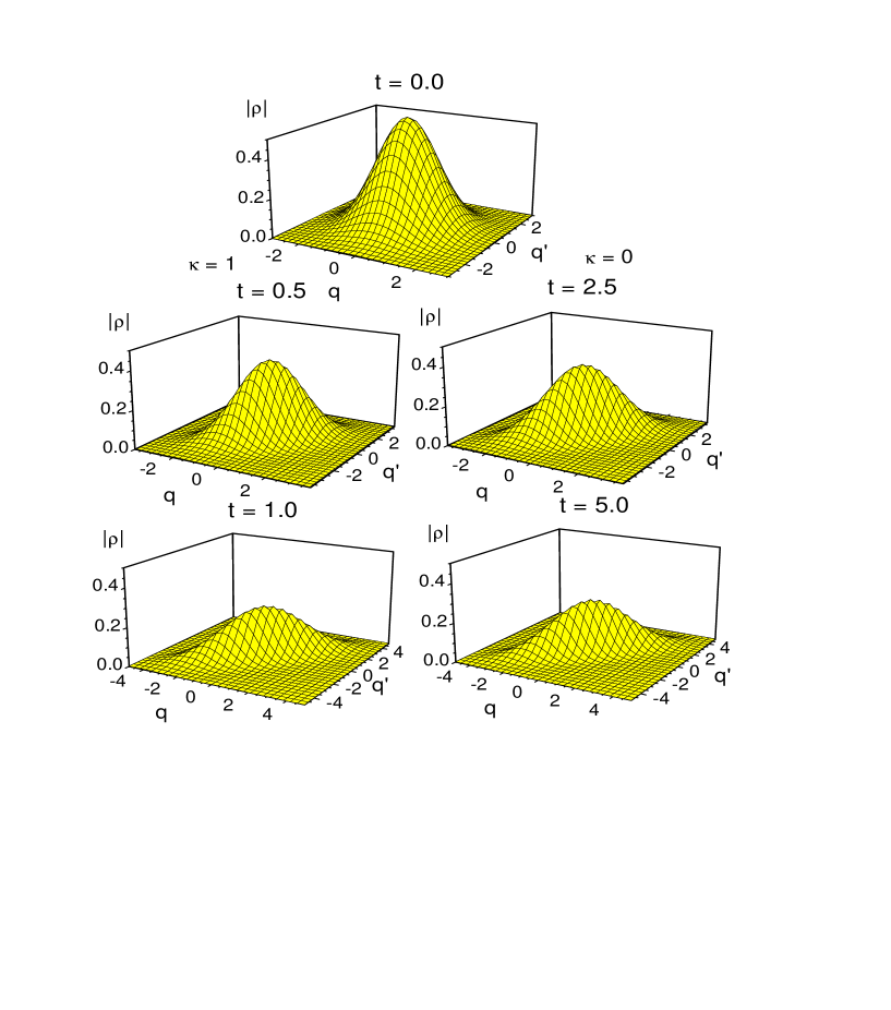
FIG. 1.: Calculated time-dependence of the module of the density matrix $|\rho(q,q^{\prime})|$ in the inverted oscillator potential, reproducing the Coulomb barrier in a ⁷⁶Ge+¹⁷⁰Er collision, for $\kappa=1$ (left side) and 0 (right side) in (56), $\lambda_{p}=(1+\kappa)\lambda$ and $\lambda_{q}=(1-\kappa)\lambda$. The parameters are $\bar{q}(0)=0$, $\bar{p}(0)=0$, $\hbar\omega=\hbar\omega_{eff}=2.0$ MeV, $\sigma_{qq}(0)=0.7$ fm², $m=53m_{0}$ ($m_{0}$ is the mass of nucleon), $\hbar\lambda=2$ MeV and $T=0$ MeV. The initial density matrix is presented on the top. The time is given in units of $6.582\times 10^{-22}$ s.

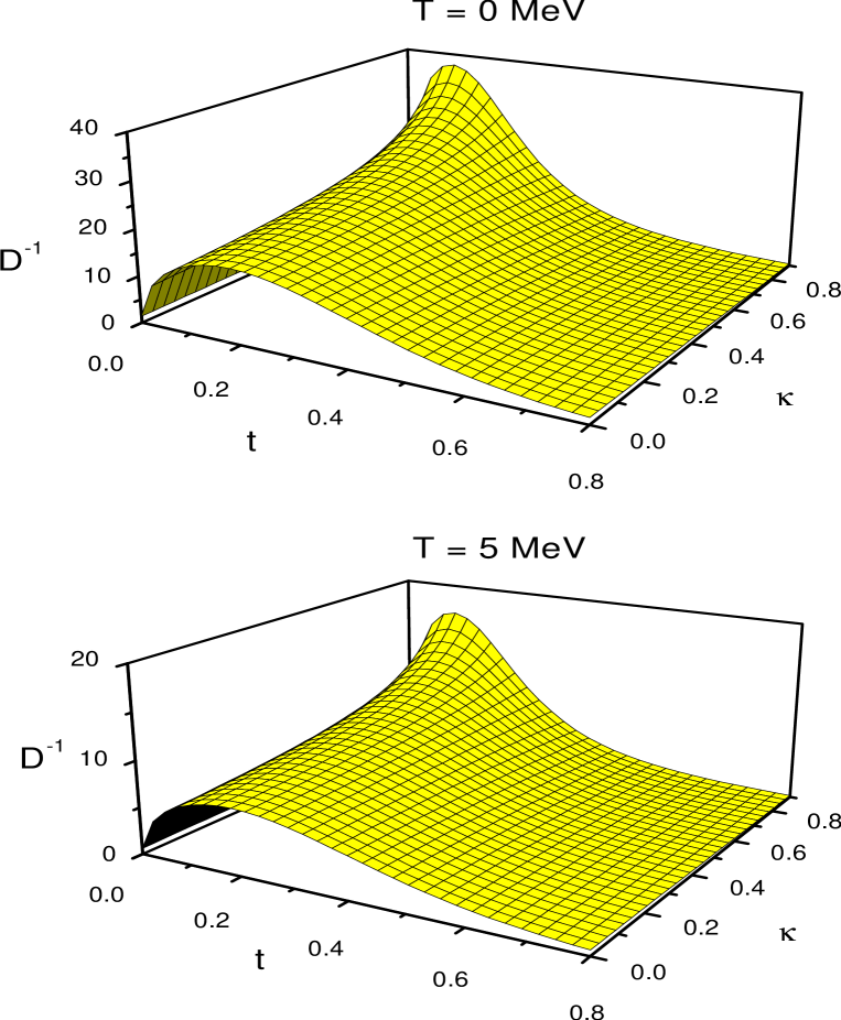
FIG. 2.: Dependence of the inverse decoherence $D^{-1}$ (units $\hbar^{-1/2}$) on time and $\kappa$, used in the definitions of $D_{pp}$ and $D_{qq}$ in (56), $\lambda_{p}=(1+\kappa)\lambda$ and $\lambda_{q}=(1-\kappa)\lambda$ at $T=0$ and 5 MeV. The initial values are $q(0)-q^{\prime}(0)=0.01$ fm and $p(0)=p^{\prime}(0)=0$. The other parameters are the same as in Fig.1. The time is given in units of $6.582\times 10^{-22}$ s.

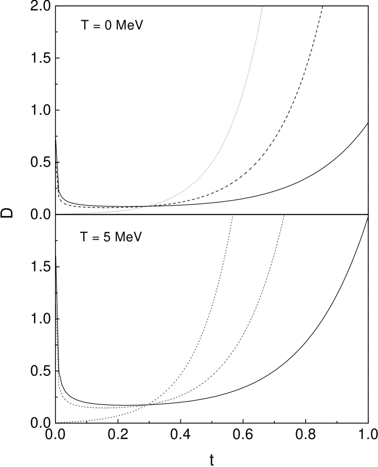
FIG. 3.: Time-dependence of the decoherence $D$ (units $\hbar^{1/2}$) for $\lambda_{p}=2\lambda$, $\lambda_{q}=0$, $T=0$ and 5 MeV, and $\kappa=0$ (solid lines), 0.5 (dashed lines) and 1 (dotted lines). The initial values are $q(0)-q^{\prime}(0)=0.01$ fm and $p(0)=p^{\prime}(0)=0$. The other parameters are the same as in Fig.1. The time is given in units of $6.582\times 10^{-22}$ s.

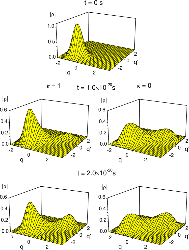
FIG. 4.: Calculated time-dependence of the module of the density matrix $|\rho(q,q^{\prime})|$ in a double-well potential (see text) for $\kappa=1$ (left side) and 0 (right side) in (56) at $T=0$ MeV and $\lambda_{p}=2\lambda$, $\lambda_{q}=0$. The initial Gaussian distribution (top part) with $\sigma_{qq}(0)=0.14$ fm², $\bar{p}(0)=0$ starts with $\bar{q}=-1.5$ fm in the left well. The further parameters are $\hbar\omega_{eff}=2.0$ MeV, $\hbar\lambda=2$ MeV and $m=53m_{0}$. The time is indicated.

REFERENCES

• [1] Lindblad G. 1976 Commun. Math. Phys. 48 119; 1976 Rep. on Math. Phys. 10 393
• [2] Belavin A.A., Zel’dovich B.Ya., Perelomov A.M. and Popov B.S. 1969 JTEP 56 264
• [3] Davies E.B. 1976 Quantum theory of open systems (New York: Academic Press)
• [4] Dodonov V.V. and Man’ko V.I. 1983 in Group Theoretical Methods in Physics, Vol. 2, ed. M.A.Markov (Nauka, Moscow)
• [5] Dodonov V.V. and Man’ko V.I. 1989 Reports of Physical Institute 167 (1986) 7; 191 171
• [6] Dekker H. 1981 Phys. Rep. 80 1
• [7] Sandulescu A. and Scutaru H. 1987 Ann. Phys. (N.Y.) 173 277
• [8] Isar A., Sandulescu A., Scutaru H., Stefanescu E. and Scheid W. 1994 Intern. J. Mod. Phys. A 3 635; Isar A., Sandulescu A. and Scheid W. 1993 J. Math. Phys. 34 3887
• [9] Antonenko N.V., Ivanova S.P., Jolos R.V. and Scheid W. 1994 J. Phys. G: Nucl.Part.Phys. 20 (1994) 1447
• [10] Strunz W.T.  1997 J. Phys. A: Math. Gen. 30 4053
• [11] Adamian G.G., Antonenko N.V. and Scheid W. 1998 Phys. Lett. A 244 482
• [12] Adamian G.G., Antonenko N.V. and Scheid W. 1999 Nucl. Phys. A 645 376
• [13] Fujikawa K., Iso S., Sasaki M. and Suzuki H. 1992 Phys. Rev. Lett. 68 1093
• [14] Weiss U. 1992 Quantum dissipative systems (Singapore: World Scientific)
• [15] Razavy M. and Pimpale A. 1988 Phys. Rep. 168 305
• [16] Caldeira A.O. and Leggett A.J. 1981 1981 Phys. Rev. Lett. 46 211; 1983 Ann. Phys. 149 374; Leggett A.J. 1984 Phys. Rev. B 30 1208
• [17] Bruinsma R. and Per Bak 1986 Phys. Rev. Lett. 56 420
• [18] Bulgac A., Dang Do G. and Kusnezov D. 1998 Phys. Rev. E 58 196
• [19] Papadopoulos G.J. 1990 J. Phys. A: Math. Gen. 23 935
• [20] Dodonov V.V. and Nikonov D.E. 1991 J. of Soviet Laser Research 12 461
• [21] Baskoutas S. and Jannussis A. 1992 J. Phys. A: Math. Gen. 25 L1299
• [22] Hofmann H. 1997 Phys. Rep. 284 137
• [23] Adamian G.G., Antonenko N.V. and Scheid W. 1999 Phys. Lett. A 260 39
• [24] Harris E.G. 1990 Phys. Rev. A 42 3685
Refer to caption