Instantons in the working memory: implications for schizophrenia.

Abstract

The influence of the synaptic channel properties on the stability of delayed activity maintained by recurrent neural network is studied. The duration of excitatory post-synaptic current (EPSC) is shown to be essential for the global stability of the delayed response. NMDA receptor channel is a much more reliable mediator of the reverberating activity than AMPA receptor, due to a longer EPSC. This allows to interpret the deterioration of working memory observed in the NMDA channel blockade experiments. The key mechanism leading to the decay of the delayed activity originates in the unreliability of the synaptic transmission. The optimum fluctuation of the synaptic conductances leading to the decay is identified. The decay time is calculated analytically and the result is confirmed computationally.

I INTRODUCTION

Long-term memory is thought to be stored in biochemical modulation of the inter-neuron synaptic connections. As each neuron forms about $10^{4}$ synapses such a mechanism of memory seems to be very effective, allowing potentially the storage of $>10^{4}$ bits per neuron. However, although the synaptic modifications persist for a long time, it may take as long as minutes to form them. Since the external environment operates at much shorter time scales, the synaptic plasticity is virtually useless for the short-term needs of survival. Such needs are satisfied by the working memory (WM), which is stored in the state of neuronal activity, rather than in modification of synaptic conductances (Miyashita, 1988; Miyashita and Chang, 1988; Sakai and Miyashita, 1991; Funahashi et al., 1989; Goldman-Rakic et al., 1990; Fuster, 1995).

WM is believed to be formed by recurrent neural circuits (Wilson and Cowan, 1972; Amit and Tsodyks, 1991a, b; Goldman-Rakic, 1995). A recurrent neural network can have two stable states (attractors), characterized by low and high firing frequencies. External inputs produce transitions between these states. After transition the network maintain high or low firing frequency during the delay period. Such a bipositional “switch” can therefore store one bit of information.

During the last few years it has become clear that NMDA receptor is critically involved in the mechanism of WM. It is evident from the impairments of the capacity to perform the delayed response task produced by the receptor blockade (Krystal et al., 1994; Adler et al., 1998, Pontecorvo et al., 1991; Cole et al., 1993; Aura et al., 1999). Similarly the injection of the NMDA receptor antagonists brings about weakening of the delayed activity demonstrated in the electrophysiological studies (Javitt et al., 1996, Dudkin et al., 1997a). At the same time intracortical perfusion with glutamate receptor agonists both improves the performance in the delayed response task and increases the duration of WM information storage (Dudkin et al., 1997a and b). Such evidence is especially interesting since administration of NMDA receptor antagonists (PCP or ketamine) reproduces many of the symptoms of schizophrenia including the deficits in WM.

Out of many unusual properties of NMDA channel two may seem to be essential for the memory storage purposes: the non-linearity of its current-voltage characteristics and high affinity to the neurotransmitter, resulting in long lasting excitatory post synaptic current (EPSC). The former have been recently implicated in being crucial for WM (Lisman et al., 1998). It was shown that by carefully balancing NMDA, AMPA, and GABA synaptic currents one can produce an N-shaped synaptic current-voltage characteristic, which complemented by the recurrent neural circuitry results in the bistability. This approach implies therefore that a single neuron can be bistable and maintain a stable membrane state corresponding to high or low firing frequencies (Camperi and Wang, 1998). Such a bistability therefore is extremely fragile and can be easily destroyed by disturbing the balance between NMDA, GABA or AMPA conductances. This may occur in the experiments with the NMDA antagonist.

The single neuron bistability should be contrasted to a more conventional paradigm, in which the bistability originates solely from the network feedback. It is based on the non-linear relation between the synaptic currents entering the neuron and its average firing rate (Amit and Tsodyks, 1991a, b; Amit and Brunel, 1997). Such a mechanism is not sensitive to the membrane voltage and therefore can be realized using e.g. AMPA receptor. Thus it may seem that this mechanism is ruled out by the NMDA antagonist experiments.

In this paper we study how the properties of the synaptic receptor can influence the behavior of the conventional bistable network. We therefore disregard the phenomena associated with the non-linearity of synaptic current-voltage relation (Lisman et al., 1998). In effect we study the deviations from the mean-field picture suggested earlier (see e. g. Amit and Tsodyks, 1991a, b). The main result of this paper concerns the question of stability of the high frequency attractor. This state is locally stable in the mean-field picture, i. e. small synaptic and other noises cannot kick the system out of the basin of attraction surrounding the state. However this state is not guaranteed to be globally stable. After a certain period of time a large fluctuation of the synaptic currents makes the system reach the edge of the attraction basin and the persistent memory state decay into the low frequency state. We therefore find how long can the working memory be maintained, subject to the influence of noises.

Before the network reaches the edge of attraction basin it performs an excursion into the region of parameters which is rarely visited in usual circumstances. This justifies the use of term “instanton” to name such an excursion, emphasizing the analogy with the particle traveling in the classically forbidden region in quantum mechanics. Such analogy have been used before in application to the perception of ambiguous signals by Bialek and DeWeese, 1995. The present study however is based on microscopic picture, deriving the decay times from the synaptic properties.

In the most trivial scenario the network can shut itself down by not releasing neurotransmitter in a certain fraction of synapses of all neurons. Thus all the neurons cross the border of attraction basin simultaneously. This mechanism of memory state decay is shown to be ineffective. Instead the network chooses to cross the border by small groups of neurons, taking advantage of large combinatorial space spanned by such groups. The cooperative nature of decay in this problem is analogous to some examples of tunneling of macroscopic objects in condensed matter physics (Lee and Larkin, 1978; Levitov et al., 1995).

The decay time of the memory state evaluated below increases with the size of the network growing (see Section III). This is a natural result since in a large network the relative strength of noise is small according to the central limit theorem. Therefore if one is given the minimum time during which the information has to be stored, there is the minimum size of the network that can perform this task. We calculate therefore the minimum number of neurons necessary to store one bit of information in a recurrent network. This number weakly depends on the storage time and for the majority of realistic cases is equal to 5-15.

Two complimentary measures of WM stability, the memory decay time and the minimum number of neurons, necessary to store one bit, are shown below to depend on the synaptic channel properties. The former grows exponentially with increasing duration of EPSC, which is unusually large for the NMDA channel due to high affinity to glutamate. This allows to interpret the NMDA channel blocking experiments in the framework of conventional network bistability.

In recent study Wang, 1999 considered a similar problem for the network subjected to the influence of external noises, disregarding the effects of finiteness of the probability of neurotrasmitter release. In our work we analyze the effects of synaptic failures on the stability of the persistent state. We therefore consider the internal sources of noise. Our study is therefore complimentary to Wang, 1999.

Analytical calculations presented below are confirmed by computer simulations. For the individual neurons we use the modified leaky integrate-and-fire model due to Stevens and Zador, 1998, which is shown to reproduce correctly the timing of spikes in vitro. Such realistic neurons may have firing frequencies within the range 15-30Hz for purely excitatory network in the absence of inhibitory inputs (Section II). This solves the high firing frequency problem (see e.g. Amit and Tsodyks, 1991a). The resolution of the problem is based on the unusual property of the Stevens and Zador neuron, which in contrast to the simple leaky integrator has two time scales. These are the membrane time constant and characteristic time during which the time-constant changes. The latter, being much longer than the former, determines the minimum firing frequency in the recurrent network, making it consistent to the physiologically observed values (see Section II for more detail).

II DEFINITION OF THE MODEL AND ITS MEAN-FIELD SOLUTION

In this section we first examine the properties of single neuron, define our network model, and, finally solve the network approximately, using the mean-field approximation.

The Stevens-Zador (SZ) model of neuron is an extension of the standard leaky integrator (see e.g. Tuckwell, 1998). It is shown to accurately predict the spike timings in layer 2/3 cells of rat sensory neocortex. The membrane potential $V$ satisfies the leaky integrator equation with time-varying resting potential $E$ and integration time $\tau$:

$$\dot{V}=\frac{E\left(t\right)-V}{\tau\left(t\right)}+I(t).$$ (1)

Here $t$ is the time elapsed since the last spike generated, and the input current $I(t)$ is measured in volts per second. When the membrane voltage reaches the threshold voltage $\theta$ the neuron emits a spike and the voltage is reset to $V_{reset}$.

(a)

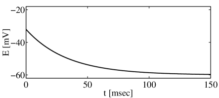
(b)

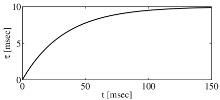
FIG. 1.: The somatic membrane resting potential (a) and the integration time (b) as functions of the time elapsed since the last spike.

This model is quite general to describe many types of neurons, differing only by the functions $E(t)$, $\tau(t)$, and the parameters $\theta$ and $V_{reset}$. For the pyramidal cells in cortical layer 2/3 of rats the functions can be fitted by

$$E\left(t\right)=E_{0}-\Delta E\left[1-\exp\left(-\alpha t/\tau_{0}\right)\right]$$ (2)

and

$$\tau\left(t\right)=\tau_{0}\left[1-\exp\left(-\alpha t/\tau_{0}\right)\right].$$ (3)

The parameters of the model for these cells have the following numerical values: $E_{0}=-32$mV, $\Delta E=28$mV, $\alpha=0.3$, $\tau_{0}=10$msec, $\theta=-22$mV, and $V_{reset}=-32$mV (Stevens and Zador, 1998). The resting potential and integration time with these parameters are shown in Figure 1.

In the next step we calculate the transduction function $f=T(I)$, relating the average external current to the average firing frequency. This function is evaluated in Appendix A and is shown in Figure 2. The closed hand expression for this function cannot be obtained. Some approximate asymptotic expressions can be found however. For large frequencies ($f\gg\alpha/\tau_{0}=30Hz$) it is approximately given by the linear function (dashed line in Figure 2):

$$T(I)\approx g\left(I-I_{0}\right),$$ (4)

where

$$g=\frac{\alpha}{1+\alpha}\frac{1}{\left|E_{0}-\theta\right|},$$ (5)

and

$$I_{0}=\frac{\Delta E}{\tau_{0}}+\frac{\left|E_{0}-\theta\right|}{2\tau_{0}}\frac{1+\alpha}{1+2\alpha}$$ (6)

For small frequencies ($f\ll\alpha/\tau_{0}$) we obtain:

$$T(I)\approx\frac{\alpha}{\tau_{0}}\frac{1}{\ln\left[\left(\left|E_{0}-\theta\right|\right)/\left(\left|E_{0}-\theta\right|+\Delta E-\tau_{0}I\right)\right]}$$ (7)

The neuron therefore starts firing significantly when current exceeds the critical value

$$I^{*}=\frac{\left|E_{0}-\theta\right|+\Delta E}{\tau_{0}}.$$ (8)

We ignore spontaneous activity in our consideration assuming all firing frequencies below $5Hz$ to be zero. We also disregard the effects related to refractory period since they are irrelevant at frequencies $10-50Hz$.

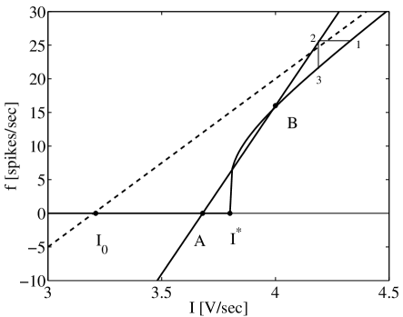
FIG. 2.: Neuronal transduction function relating the firing frequency and the input current (solid line $I_{0}AI^{*}B$). The straight line $AB$ describes the network feedback. The dashed line represents the asymptotes of the transduction function for large frequencies. It is given by Eq. (4). The expressions for $I_{0}$ and $I^{*}$ are provided by Eqs. (6) and (8). The points $A$ and $B$ are the low and high frequency attractors respectively. The numbers $123$ demonstrate the trajectory of the system approaching the high frequency attractor.

We consider the network consisting of $N$ SZ neurons, establishing all-to-all connections. After each neuron emits a spike a EPSC is generated in the input currents of all cells with probability $\kappa$. This is intended to simulate the finiteness of probability of the neurotransmitter release in synapse. The total input current of $n$-th neuron is therefore

$$I_{n}(t)=\sum_{k=1}^{N}\sum{s_{k}}b_{n,s_{k}}j(t-t_{s_{k}})+I_{n}^{ext}(t),$$ (9)

where $k$ enumerates the neurons making synapses on the $n$-th neuron (all neurons in the network), $t_{s_{k}}$ is the time of spike number $s_{k}$ emitted by cell $k$, and $I_{n}^{ext}$ is the external current. $b$ is a boolean variable equal to $1$ with probability $\kappa$ (in our computer simulations always equal to 0.3). It is the presence of this variable that distinguishes our approach from Wang, 1999. We chose the EPSC represented by $j(t)$ to be (see Amit and Brunel, 1997)

$$j=j_{0}\exp(-t/\tau_{{}_{\rm EPSC}})H(t),$$ (10)

where $H(t)=1$, if $t>0$, and $H(t)=0$ otherwise. As evident from (10) $\tau_{{}_{\rm EPSC}}$ is the duration of EPSC. It is therefore the central variable in our consideration.

If the number of neurons in the network is large its dynimics is well described by the mean-field approximation. How large the number of neurons should be is discussed in the next Section. For the purposes of mean-field treatment it is sufficient to use the average firing frequency $\bar{f}$ and the average input current $\bar{I}$ to describe the network completely. Thus the network dynamics can be approximated by one “effective” neuron receiving the average input current and firing at the average frequency. Assume that this hypothetical neuron emits spikes at frequency $f(t)$ (point 1 in Figure 2). Due to the network feedback this results in the input current equal to the average of Eq. (9), displaced in time by the average duration of EPSC, i.e.

$$I(t+\tau_{{}_{\rm EPSC}})\approx\bar{I}=N\kappa j_{0}\tau_{{}_{\rm EPSC}}\bar{f}(t)+\bar{I}^{ext}.$$ (11)

This corresponds to the transition between points 1 and 2 in Figure 2. At last the transition between the input current and the firing frequency is accomplished by the transduction function $T(I)$ (points 2 and 3). The delay due to this transition is of the order of somatic membrane time constant ($\sim 10$msec) and is negligible compaed to $\tau_{{}_{\rm EPSC}}\sim 100$msec. We therefore obtain the equation on the firing frequency $\bar{f}(t+\tau_{{}_{\rm EPSC}})=T\left(\bar{I}(\bar{f}(t))\right)$ (Wilson and Cowan, 1972), or using the Taylor expansion

$$\tau_{{}_{\rm EPSC}}\dot{\bar{f}}=T(\bar{I}(\bar{f}))-\bar{f}.$$ (12)

To obtain the steady state solutions we set the time derivatives in (12) to zero

$$T(I)=I^{-1}(I).$$ (13)

Here $I^{-1}(I)$ is the function inverse to (11). It is shown in Figure 2 by the straight solid line. This equation has three solutions, two of which are stable. They are marked in by letters $A$ and $B$ in the Figure.

Point $B$ represents the high frequency attractor. Frequencies obtained in SZ model neurons are not too high. They are of the order of $\alpha/\tau_{0}$, i.e. in the range $15-30$ Hz. This coinsides with the range of frequencies observed in the delayed activity experiments (Miyashita, 1988; Miyashita and Chang, 1988; Sakai and Miyashita, 1991; Funahashi et al., 1989; Goldman-Rakic et al., 1990; Fuster, 1995). The reason for the relatively low firing frequency rate is as follows. For the leaky integrator model the characteristic firing rates in the recurrent network are of the order of $1/\tau$, i. e. are in the range $50-100$Hz. For the SZ neuron $\tau$ is even smaller (see Figure 1b), and therefore it seems that the firing rates should be larger than for leaky intergator. This however is no true, since for the SZ neuron, in contrast to the leaky integrator, there is the second time scale. It is the characteristic time of variation of the time constant $\tau_{0}/\alpha\sim 30-50$ msec (see Figure 1b). Since the time constant itself is very short it becomes irrelevant for the spike generation purposes at low firing rates and the second time scale determines the characteristic frequency. It is therefore in the range $15-30$Hz.

Finally we would like to discuss the stability of attactor $B$. It can be locally stable, i.e. small noises cannot produce the transition from state $B$ to state $A$. The condition for this follows from the linerized near equilibrium Eq. (12):

$$\nu=\frac{dT}{d\bar{I}}\frac{d\bar{I}}{d\bar{f}}<1$$ (14)

Very rarely, however, a large fluctuation of noise can occur, that kicks the system out of the basin of attraction of state $B$. It is therefore never globally stable. This is the topic of the next Section.

III BEYOND MEAN-FIELD APPROXIMATION

Computer simulations show that our network can successfully generate delayed activity response. An example is shown in Figure 3a where a short pulse of external current (dashed line) produced transition to the high frequency state. This state is well described by the mean-field treatment given in the previous section. This is true, however, only for the networks containing a large number of neurons $N$. If the size of the network is smaller than some critical number $N^{*}$ the following phenomenon is observed (see Figure 3b). The fluctuations of the current reach the edge of the attraction basin (dotted line) and the network abruptly shuts down, jumping from high frequency to the low frequency state. The quantitative treatment of these events is the subject of this section.

(a)

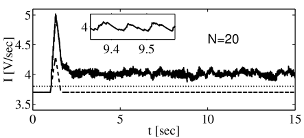
(b)

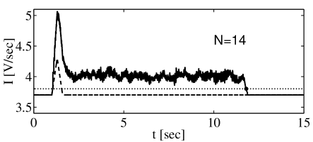
FIG. 3.: Total input current averaged over all the neurons in the network. A short pulse of the external current brings about the transition to the high frequency state, in which the total current is larger than the external current due to the feedback. (a) In large networks (N=20) the delayed activity can persist virtually forever, until the external inputs are changed. The inset shows the traces of neuronal synchronization: the average current experiences oscillations at the average firing frequency. (b) In small network (N=14) the high frequency state can decay and the delayed activity disapear. This results in the average current crossing the edge of the attraction basin, trace of which is shown by the dotted line.

Similar decay processes have been observed by Funahashi et al., 1989 in prefrontal cortex. One of the examples of such error trials is shown in Figure 4.

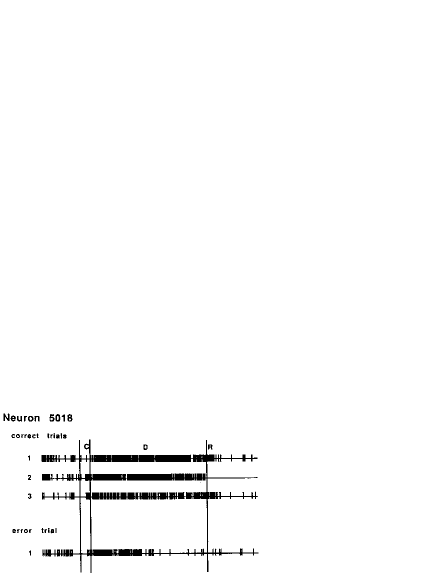
FIG. 4.: Sudden decay of the dalayed activity in the neuron in prefrontal cortex during error trial (bottom figure) observed by Funahashi et al., 1989.

Although the decay is abrupt, the moment at which it occurs is not reprodusable from experiment to experiment. It is of interest therefore to study the distribution of the time interval between the initiation of the delayed activity and the moment of its decay. Our simulations and the arguments given in Appendix B show that the decay can be considered a Poisson process. The decay times have therefore an exponential distribution (see Figure 5).

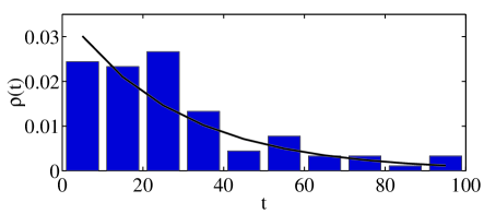
FIG. 5.: The density of probability of decay at time $t$ obtained in the numerical experiment (bars) and the exponential distribution with $\bar{t}=28$sec (solid curve). The latter is given by Eq. (B8). The numerical results are include 100 trials with $\bar{f}\approx 16$Hz, $N=14$, $\tau_{{}_{\rm EPSC}}=80$msec.

Since failure to maintain the persistent activity entails the loss of the memory and incorrect performance in the delayed responce task, at least in monkey’s prefrontal cortex (Funahashi et al., 1989), one can use the conclusion about Poisson distribution to interpret some psychophysical data. In some experiments on rats performing the binary delayed matching to position tasks deterioration of WM is observed as a function of delay time (Cole et al., 1993). The detereoration was characterized by “forgetting” curve, with matching accuracy decreasing from about 100% at zero delay to approximately 70% at 30 second delay. The performance of the animal approaches the regime of random guessing with 50% of correct responses in this binary task (Figure 6). Our prediction for the shape of the “forgetting” curve that follows from the Poisson distribution of delayed activity times is

$$Correct=(1+\exp(-t/\bar{t}))/2\times 100\%.$$ (15)

This prediction is used to fit the experimental data in Figure 6.

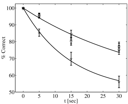
FIG. 6.: The performance of rats in delayed matching to position task (from Cole et al., 1993). Different markers show various degrees of sedation with competitive NMDA antagonist CPP: circles 0 mg/kg; triangles 1 mg/kg; hexagons 3 mg/kg; pentagons 10 mg/kg. The solid lines represent the fits by Eq. (15). The upper and lower lines correspond to the average decay times 40 and 15 seconds respectively.

This Figure also shows the effect of competitive NMDA antagonist CPP. Application of the antagonist reduces the average memory retention time $\bar{t}$ from about 40 seconds to 15 seconds. The presence of non-compatitive antagonists impairs performance even at zero delay (Cole et al., 1993; Pontecorvoet al., 1991). Non-competitive antagonists have therefore an effect on the components of animal behavior different from WM. When the delayed component of “forgetting” curve is extracted it can be well fitted by an expression containing exponential similar to (15). Such fits also show that the average WM storage time $\bar{t}$ decreases with application of NMDA antagonist.

Our calculation in Appendix B show that the average memory storage time is given by

$$\bar{t}\sim\tau_{{}_{\rm EPSC}}\exp\left[{\kappa f\tau_{{}_{\rm EPSC}}N^{2}\left(\Delta I/I\right)^{3}}\right].$$ (16)

Here $\Delta I$ is the distance to the edge of the attraction basin from the stable state and $I$ is the average feedback current. This result holds if $f\tau_{{}_{\rm EPSC}}\gg 1$. Because $\bar{t}$ is of the order of tens of seconds and $\tau_{{}_{\rm EPSC}}$ is approximately $100$ msec the exponential in (16) is of the order of $10^{2}$-$10^{3}$ for the realistic cases.

There are therefore two ways how synaptic receptor blockade can affect $\bar{t}$. First, the attenuation of the EPSC decreases the average firing frequency $f$. Second, it moves the system closer to the edge of the attraction basin, reducing $\Delta I$. Both factors increase the effect of noise onto the system, decreasing the average memory storage time. This is manifested by Eq. (16).

Another consequence of the formula is the importance of NMDA receptor for the WM storage. It is based on the large affinity of the receptor to glutamate, leading to long EPSC ($\tau_{{}_{\rm NMDA}}\approx 100$ msec), compared for example to AMPA receptor ($\tau_{{}_{\rm AMPA}}\approx 15$ msec). Eq. (16) implies that if AMPA receptor is used in the bistable neural net and all other parameters ($\kappa$, $f$, $N$, and $\Delta I/I$) are kept the the same, the memory storage time is equal to $\tau_{\rm AMPA}\approx 15$ msec. Thus it is not suprising that NMDA receptor is chosen by evolution as a mediator of WM and the highest density of the receptor is observed in places involved into the WM storage, i.e. in prefrontal cortex (Cotman et al., 1987).

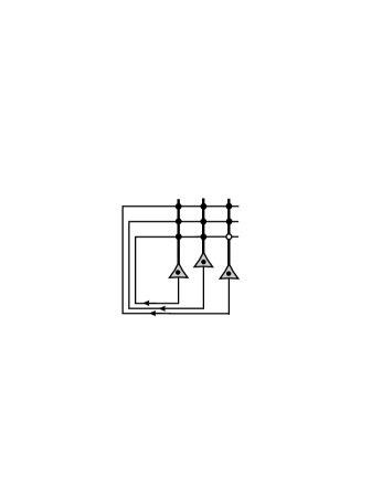
FIG. 7.: The network used in text to illustrate the optimum fluctuation leading to the delayed activity decay. The synapses are shown by circles. The synapses releasing neurotransmitter are shown by full circles. The failing synapse is shown by the open circle. The dendrites and axons are represented by thick and thin lines respectively.

We now would like to illustrate what processes lead to the decay time given by (16). Consider a simple network consisting of three neurons (Figure 7). Assume that the ratio $\Delta I/I$ for this network is equal to 1/3. This implies that the neurons have to lose only 1/3 of their recurrent input current due to a fluctuation to stop firing. This can be accomplished by various means. Our research shows that the most effective fluctuation is as follows. Due to probabilistic nature of synaptic transmition some of the synapses release glutamate when spike arrives onto the presinaptic terminal (full circles in Figure 7) some fail to do so (open circle). It is easy to see that if the same synapse fails to release neurotransmitter in responce to any spike arriving during the time interval $\tau_{{}_{\rm EPSC}}$ the reverberations of current terminate. Indeed, the failing synapse (open circle) deprives the neuron of 1/3 of its current. This is just enough to put the input current into the neuron below the threshold. The neuron therefore stops firing. This deprives the entire network, consisting of three neurons, of 1/3 of its feedback current. Therefore the delayed activity in this network terminates.

In the the most reasonable alternative mechanism of decay the average mean-field current would reach the edge of the attraction basin i.e. would be reduced by 1/3. This can be accomplished by shutting down three synapses in three different neurons instead of one. Such mechanism is therefore less effective than the proposed above. Quantitatively the difference is manifested in reducing the exponent of the factor containg $\Delta I/I<1$ in Eq. (16) from 3 to 2. This bring about an increase in the average storage time. The mean-field mechanism is therefore less restrictive than the proposed one and is disregarded in this paper.

Since an increase of the number of neurons in the network $N$ dramatically influences the memory storage time according to Eq. (16), another characteristic of the reliability of WM circuit is the minimum number of neurons $N^{*}$ necessary to store one bit of information during time $\bar{t}$. We first study this quantity computationally as follows. We run the network simulation many times with the same values of $N$ and $\tau_{{}_{\rm EPSC}}$. We then determine the average decay time $\bar{t}$. Having done this we decrease or increase $N$ depending on wheater $\bar{t}$ is larger or smaller than a given value (20 sec in all our simulations). This process converges to the number of neurons necessary to sustain the delayed activity $N^{*}$ for the given value of $\tau_{{}_{\rm EPSC}}$. The process is then repeated for different values of synaptic time-constant. However, the network feedback is always renormalized so that the firing frequency stays the same, close to the physiologically feasible value $\bar{f}\approx 16Hz$. This corresponds to the attractor state shown in Figure (2). The resulting dependence of $N^{*}$ versus $\tau_{{}_{\rm EPSC}}$ is shown in Figure 8 by markers.

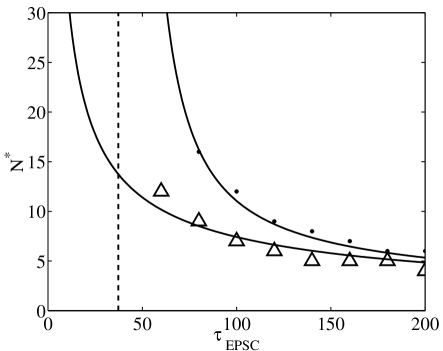
FIG. 8.: The minimum number of neurons $N^{*}$ needed to maintain delayed activity with average decay time 20 sec for $\bar{f}\approx 16$Hz. The dots show computational results for the case of no noise in the external inputs. The triangles correspond to the case of 10% white noise added to the external current. The solid lines represent the result of analytical calculation described below in the text. The dashed line is the vertical asymptote of $N^{*}$ for the case of no external noise. No delayed activity can exist to the left of this line, i.e. for the synaptic receptor time constant smaller than 37 msec.

There are two sets of computational results in Figure 8. The higher values of $N^{*}$ are obtained for the network with no noise in the external inputs (dots in Figure 8). The only source of noise in such a network is therefore the unreliability of synaptic connections. It appears for this case that no delayed activity can exist for $\tau_{{}_{\rm EPSC}}$ below 37 msec. The lower values of $N^{*}$ are obtained for the case of white noise added to the external input (triangles). The amplitute of white noise is $10\%$ of the total input current and the correlation time is 1 msec. The limiting value of synaptic time constant for which the dalayed activity is not possible is much smaller for this case ($\approx 5$ msec).

This result may seem counter-intuitive. Having added the external noise we increased the viability of the high frequency state, reducing the effects of the internal synaptic noise. This however is not so suprising if one takes the neuronal synchrony into account. Synchrony of neuronal firing results in oscillations in the average input current (see inset in Figure 2a). Such oscillations periodically bring the system closer to the edge of the attraction basin, creating additional opprotunities for decay. Thus the syncronous network is less stable than the asynchronous one. External noice attenuates neuronal synchrony, smearing the ascillations of the average input current. Thus the system with noise in the external inputs should have a larger decay time and smaller critical number of neurons $N^{*}$. This idea is discussed quantitatively below in this Section. This is similar to the stabilisation of the mean-field solutions in the networks of pulse-coupled oscillators (Abbott and Vreeswijk, 1993).

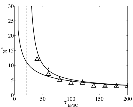
FIG. 9.: The minimum number of neurons $N^{*}$ needed to maintain delayed activity with average decay time 20 sec for the attaractor with average firing frequency 28 Hz. Notations are the same as in Figure 8. The cut-off value of synaptic time constant is 27 msec. The numerical results with external noise in this case are slightly above the theoretical prediction due to insufficient suppression of synchrony.

Figure 9 shows the results of similar calculations for the attractor state with a higher average firing frequency ($\bar{f}=28$Hz). This network shows higher reliability and smaller values of $N^{*}$ for both synchronous and asyncronous (10% noise added) regimes. This is consistent with Eq. (16). The results of analytical calculations (solid lines) show satisfactory agreement with the computer modeling (markers). The rest of the Section is dedicated to the discussion of different aspects of the analytical calculations and their results. A more thorough treatment of the problem can be found in Appendix B.

To evaluate the minimum number of neurons in the closed hand form we solve Eq. (16) for $N$

$$N^{*}\approx N_{1}^{*}\equiv\frac{1}{\sqrt{\kappa f\tau_{{}_{\rm EPSC}}}}\left(\frac{I}{\Delta I}\right)^{3/2}\sqrt{\log\left(\frac{\bar{t}}{\tau_{{}_{\rm EPSC}}}\right)}$$ (17)

This equation is valid for $f\tau_{{}_{\rm EPSC}}\gg 1$. In the opposite case $f\tau_{{}_{\rm EPSC}}\lesssim 1$ it has to be amended. To obtain the correct expression in the latter case the following considerations should be taken into account.

A Fluctuations of the average mean-field current.

It is obvious that when the mean-field attractor becomes less and less stable in the local sense, i.e. the dimensionless feedback coefficient $\nu<1$ [Eq.(14)] approaches unity, the global stability should also suffer. Indeed, if the system is weakly locally stable the fluctuations in the average current are large. This should facilitate global instability. The facilitation can be accounted for by noticing that the transition from high frequency state $B$ to the low frequency one $A$ is most probable when the average current is low. Hence to obtain the most realistic probability of transition and correct values for $\bar{t}$ and $N^{*}$ one has to decrease the values of average current and distance to the edge of the attraction basin by

$$\begin{array}[]{l}{\displaystyle I\rightarrow I-\delta I,}\\ \\ {\displaystyle\Delta I\rightarrow\Delta I-\delta I,}\end{array}$$ (18)

where the standard deviation of the average current $\delta I$ is calculated in Appendix B

$$\delta I=\frac{I}{N\sqrt{2(1-\nu)\kappa f\tau_{{}_{\rm EPSC}}}}.$$ (19)

Here $I$ is the average current before the shift. This correction decreases the ratio $\Delta I/I$, decreasing $\bar{t}$ [see Eq. (16)]. This implies the reduced reliability of the network due to the average current fluctuations.

B Large combinatorial space covered by small groups of neurons attempting to cross the attraction basin edge.

In the simple example with three neurons, in principle, each of them can contribute to the process of decay. If the network is larger the number of potentially dangerous groups grows as a binomial coefficient $C_{N}^{n}$, where $n=N\Delta I/I\leq N$ is the size of the dangerous group. The correction to $N^{*}$ can be expressed as follows (Appendix B):

$$N^{*}=\sqrt{\left(N_{1}^{*}\right)^{2}+\left(N_{2}^{*}\right)^{2}}+N_{2}^{*}.$$ (20)

Here $N_{2}^{*}$ is the combinatorial correction

$$N_{2}^{*}=\left(\frac{I}{\Delta I}\right)^{3}\frac{\phi\left(\Delta I/I\right)+\left(\Delta I/I\right)\ln A}{\kappa f\tau_{{}_{\rm EPSC}}}.$$ (21)

Here

$$\begin{array}[]{l}{\displaystyle A=\frac{I}{\Delta I\sqrt{4\pi N^{*}\kappa f\tau_{{}_{\rm EPSC}}}},}\\ \\ {\displaystyle\phi(x)=x\ln\left[1/x\right]+(1-x)\ln\left[1/(1-x)\right].}\end{array}$$ (22)

Since the combinatorial contribution $N_{2}^{*}$ is proportional to $1/f\tau_{{}_{\rm EPSC}}$ it is negligible compared to $N_{1}^{*}\propto 1/\sqrt{f\tau_{{}_{\rm EPSC}}}$ at large values of $\tau_{{}_{\rm EPSC}}$. Therefore $N^{*}\approx N_{1}^{*}$ as claimed by Eq. (17) in this limit. On the other hand if $\tau_{{}_{\rm EPSC}}$ is small the main contribution to the critical number of neurons $N^{*}$ comes from $N^{*}_{2}$.

The right hand sides of Eqs. (17) and 21 contains dependence on $N^{*}$ through the shift in distance to the attraction edge $\delta I$ and the coefficient $A$. This dependence is weak however since the former represents a very small correction and the latter depends on $N^{*}$ only logarithmically. Nevertheless to generate a numerically precise prediction we iterate Eq. (17), (20), and (17) until a consistent value of $N^{*}$ is reached. The results are shown by lower solid lines in Figures 8 and 9. They are in a good agreement with numerical simulations in which the synchrony of firing was suppressed by external noise.

C Neuronal synchrony.

The synchronizaton of neuronal firing can be critical for the stability of the high frequency attractor. Consider the following simple example (Wang, 1999). Consider the network consisting on only one neuron. Assume that the external input current to the neuron exceeds the firing threshold $I^{*}$ at certain moment and the neuron starts emiting spikes. Assume that the external current is then decreased to some value below the threshold. The only possibility for the neuron to keep firing is to receive enough feedback current from itself, so that the total input current is above threshfold. Suppose then for illustration purposes that the synapse that the neuron forms on itself (autapse) is infinitely reliable, i.e. every spike arriving on the presynaptic terminal brings about the release of neurotransmitter. It is easy to see that if the duration of EPSC is much shorter than the interspike interval the persistent activity is impossible. Indeed, if EPSC is short, at the moment, when the new spike has to be generated there is almost no residual EPSC. The input current at that moment is almost entirely due to external sources, i.e. is below the threshold. The new spike generation is therefore impossible. We conclude that the persistent activity is impossible if EPSC is short, i. e. for $f\tau_{{}_{\rm EPSC}}\ll 1$. Note, that this conclusion is made assuming no noise in the system.

The natural question is why this conclusion is relevant to the network consisting of many neurons? Our computer modeling shows that in the large network the neuronal firing pattern is highly sychronized on the scales of the order of $T=1/f$. In essence all neurons fire simultaneously and periodically with the period $T$. Therefore they behave as one neuron. Hence the delayed activity in such network is impossible if $f\tau_{{}_{\rm EPSC}}\ll 1$ even in the absence of synatic noise. Thus the synchrony facilitates the decay of the delayed activity brought about by the noise. This is consistent with the results of computer simulations presented if Figures 8 and 9.

As it was mentioned above synchrony facilitates the instability by producing the oscillations in the average current and therefore by bringing the edge of the attraction basin closer. It therefore effectively decreases $\Delta I$. The magnitude of this decrease is estimated in Appendix B to be

$$\begin{array}[]{l}{\displaystyle\delta I_{syn}\approx\frac{2I}{\pi f\tau_{{}_{\rm EPSC}}}}\\ \\ {\displaystyle\times\frac{f\tau_{{}_{\rm EPSC}}-e^{-1/f\tau_{{}_{\rm EPSC}}}\left(f\tau_{{}_{\rm EPSC}}+1\right)}{1-e^{-1/f\tau_{{}_{\rm EPSC}}}}}\end{array}$$ (23)

and

$$\Delta I\rightarrow\Delta I-\delta I_{syn}.$$ (24)

Here $I$ is the average current given by (18). This correction, which is the amplitude of the oscillations of the average current due to synchrony, is in good agreement with computer modeling (see insert in in Figure 3a). The synchrony does not change the average current in the network significantly. Therefore the latter should not be shifted as in (18).

These corrections imply that if the original value of $\Delta I$ is equal to the sum $\delta I+\delta I_{syn}$ [see Eq. (19)], the effective distance to the edge of attraction basin vanishes. The delayed activity cannot be sustained under such a condition. This occurs at small values of $\tau_{{}_{\rm EPSC}}$ and determines the positions of vertical asymptotes (dashed lines) in Figures 8 and 9. This gives a quantitative meaning to the argument of impossibility of stable delayed activity in synchronous network at small values of synaptic time constant given above (see also Wang, 1999). When the synchrony is diminished by external noise, the cut off value of $\tau_{{}_{\rm EPSC}}$ is determined only by $\Delta I=\delta I$ and is therefore much smaller. It is about 5 msec in our computer similations.

Synchrony also affects the values of the critical number of neurons for large and small $f\tau_{{}_{\rm EPSC}}$ ($N^{*}_{1}$ and $N^{*}_{2}$ respectively)

$$N^{*}_{1syn}=\left(\frac{I}{\Delta I}\right)^{3/2}\frac{1}{f\tau_{{}_{\rm EPSC}}}\sqrt{\frac{2\ln\left(t/\tau_{{}_{\rm EPSC}}\right)}{\kappa\left(e^{2/f\tau_{{}_{\rm EPSC}}}-1\right)}},$$ (25)

$$N^{*}_{2syn}=\left(\frac{I}{\Delta I}\right)^{3}\frac{\phi\left(\Delta I/I\right)+\left(\Delta I/I\right)\ln A}{e^{2/f\tau_{{}_{\rm EPSC}}}-1}\frac{1}{\kappa f^{2}\tau_{{}_{\rm EPSC}}^{2}}$$ (26)

These equations are derived in Appendix B. To obtain the value of critical number of neurons $N^{*}$ Eq. (20) should be used. Let us compare the latter equations to (17) and (21). In the limit $f\gg 1$ the expressions for $N^{*}_{1}$ and $N^{*}_{1syn}$ converge to the same asymptote $N^{*}_{1}\approx N^{*}_{1syn}$, whereas both $N^{*}_{2}$ and $N^{*}_{2syn}$ go to zero.

Since again, as in asynchronous case, both $N^{*}_{1syn}$ and $N^{*}_{2syn}$ depend on the quantity that we are looking for $N^{*}$ (however, again, very weakly), an iterative procedure should be used to determine the consistent value of $N^{*}$. Having applied this iterative procedure we obtain the ipper solid lines in Figures 8 and 9. We therefore obtain an excellent agreement with the results of the numerical study. In addition we calculate the cut-off $\tau_{{}_{\rm EPSC}}$, below which the delayed activity is not possible for the synchronous case. For the attractor with $\bar{f}\approx 16$ Hz the cut-off value is $37$ msec, while for the higher frequency attractor ($\bar{f}\approx 28$ Hz) the value is $21$ msec. These values are shown in Figures 8 and 9 by dashed lines. We therefore conclude that the delayed activity mediated by AMPA receptor is impossible in the synchronous case.

IV DISCUSSION

In this work we derive the relationship between the dynamic properties of the synaptic receptor channels and the stability of the delayed activity. We conclude that the decay of the latter is a Poisson process with the average decay time exponentially depending on the time constant of EPSC. Our quantitative conclusion applied to AMPA receptor, having a short EPSC, implies that it is incapable of sustaining the persistent activity in case of synchronization of firing in the network. For the case of asynchronous network one needs a large number of neurons $>30$ to store one bit of information with AMPA receptor. On the other hand NMDA receptor seems to stay away from these problems, providing reliable quantum of information storage with about 15 neurons for both synchronized and asynchronous case. We therefore suggest an explanation to the obvious from experiments high significance of the NMDA channel for WM.

One can conclude from our study that if the time constant of NMDA channel EPSC is further increased, the WM can be stored for much longer time. Assume that $\tau_{{}_{\rm EPSC}}$ is increased by a factor of 2, for instance, by genetic enhancement (Tang et al., 1999). If the network connectivity, firing frequency, and average currents stay the same as in the wild type, the exponential in Eq. (16) is increased by a factor of $10^{3}$. This implies that the working memory can be stored by such an animal for days, instead of minutes. Alternatively the the number of neurons responsible for the storage of quantum of information can be decreased by a factor $0.7$ keeping the storage time the same. This implies the higher storage capacity of the brain of mutant animals.

We predict that with normal NMDA receptor the number of neurons able to store one bit of information for $40$ sec is about 15. Should our theory be applicable to rats performing delayed matching to position task (Cole et al., 1993) the conclusion would be that the recurrent circuit responsible for this task contains $<$ 15 neurons. Of course this would imply that other sources of loss of memory, such as distraction, are not present.

The use of very simple model network allowed us to look into the nature of the global instability of delayed activity. The principal result of this paper is that the unreliability of synaptic conductance provides the most effective channel for the delayed activity decay. We propose the optimum fluctuation of the synaptic noises leading to the loss of WM. Decay rates due to such a fluctuation agree well with the results of the numerical study (Section III). Thus any theory or computer simulation that does not take the unreliability of synapses into account does not reproduce the phenomenon exactly.

We also studied the decay process in the presence of noise in the afferent inputs. The study suggests that the effect of noise on the WM storage reliability is not monotonic. Addition of small white noise ($<10$% of the total external current) increases the reliability, by destroying synchronization. It is therefore beneficial for the WM storage. Further increase of noise ($>12$%) destroys WM, producing transitions between the low and high frequency states. We conclude therefore that there is an optimum amount of the afferent noise, which on one hand smoothes the synchrony out and on the other hand does not produce the decay of delayed activity itself. Further work is needed to study the nature of influence of the external noise in the case of unreliable synapses.

If the afferent noise is not too large the neurons fire in synchrony. The natural consequences of synchrony are the decrease of the coefficient of variation of the interspike interval for single neuron and the increase of the crosscorrelations between neurons. The latter prediction is consistent with findings of some multielectrode studies in monkey prefrontal cortex (see Dudkin et al., 1997a). On the other hand sinchrony may also be relevant to the phenomenon of temporal binding in the striate cortex (Engel et al., 1999; Roskies, 1999). We argue therefore that temporal binding with the precision of dosens of millisconds can be accomplished by formation of recurrent neural networks.

We also suggest the solution to the high firing frequency problem by using a more precise model of the spike generation mechanism, i.e. the leaky integrator model with varying in time resting potential and integration time. The minimum firing frequency for the recurrent network based on such model is determined by the rate of variation of the potential and time-constant and is within the range of physiologically observed values. Further experimental work is needed to see if the model is applicable to other types of neurons, such as inhibitory cells.

In conclusion we have studied the stability of delayed activity in the recurrent neural network subjected to the influence of noise. We conclude that the global stability of the persistent activity is affected by properties of synaptic receptor channel. NMDA channel, having a long EPSC duration time, is a reliable mediator of the delayed responce. On the other hand AMPA receptor is much less reliable, and for the case of synchronized firing in principle cannot be used to sustain responce. Effect of the NMDA channel blockade on the WM task performance is discussed.

V ACKNOLEDGEMENTS

The author is grateful to Thomas Albright, Paul Tiesinga, and Tony Zador for discussions and numerous helpful suggestions. This work was supported by the Alfred P. Sloan Foundation.

A Single-neuron transduction function

In this Appendix we calculate the single-neuron transduction function. The first step is to find the membrane voltage as a function of time. From Eq. (1) using the variation of integration constant we obtain

$$\begin{array}[]{l}{\displaystyle V(t)=V_{reset}e^{-S(t)}}\\ \\ {\displaystyle+\int_{t_{0}}^{t}dt^{\prime}e^{S(t^{\prime})-S(t)}\left[I(t^{\prime})+E(t^{\prime})/\tau(t^{\prime})\right].}\end{array}$$ (A1)

Here

$$S(t)=\int_{t_{0}}^{t}dt^{\prime}/\tau(t^{\prime}),$$ (A2)

and we introduced the refractory period both for generality and to resolve the peculiarity at $t=0$. For constant current and functions given by (2) and (3) the expression for voltage can be further simplified:

$$\begin{array}[]{l}{\displaystyle V(t)=V_{reset}e^{-S(t)}+E_{0}\left[1-e^{-S(t)}\right]}\\ \\ {\displaystyle+\left(I-\frac{\Delta E}{\tau_{0}}\right)\frac{\tau_{0}}{\alpha}\frac{L_{1/\alpha}\left(e^{\alpha t/\tau_{0}}\right)e^{-S(t)}}{\left(e^{\alpha t_{0}/\tau_{0}}-1\right)^{1/\alpha}}},\end{array}$$ (A3)

where

$$S(t)=\frac{1}{\alpha}\ln\left(\frac{e^{\alpha t/\tau_{0}}-1}{e^{\alpha t_{0}/\tau_{0}}-1}\right)$$ (A4)

and $L_{n}(x)$ is defined for integer $n$ by

$$\begin{array}[]{l}{\displaystyle L_{0}(x)=\ln(x),}\\ \\ {\displaystyle L_{n}(x)=\frac{1}{n}(x-1)^{n}-L_{n-1}(x),}\end{array}$$ (A5)

and is obtained for fractional $n$ by analytical continuation. For example

$$\begin{array}[]{l}{\displaystyle L_{1}(x)=x-1-\ln(x),}\\ \\ {\displaystyle L_{2}(x)=(x-1)^{2}/2-x+1-\ln(x),}\\ \\ {\displaystyle L_{3}(x)=(x-1)^{3}/3-(x-1)^{2}/2+x-1-\ln(x),}\\ \\ {\cdots}\end{array}$$ (A6)

Solving the equation $V(t)=\theta$ produces the interspike interval $t$ and frequency $f=1/t$. The solution cannot be done in the closed form. Some asymptotes can be calculated however. The calculation depends on the value of parameter $\xi=\alpha t/\tau_{0}$.

i) $\xi=\alpha t/\tau_{0}\ll 1$.

In this limit

$$e^{-S(t)}\approx\frac{\left(e^{\alpha t_{0}/\tau_{0}}-1\right)^{1/\alpha}}{\xi+\xi^{2}/2},$$ (A7)

is very small and can be neglected everywhere, except for when multiplied by large factor $L_{1/\alpha}$. The latter product

$$\frac{L_{1/\alpha}\left(e^{\alpha t/\tau_{0}}\right)e^{-S(t)}}{\left(e^{\alpha t_{0}/\tau_{0}}-1\right)^{1/\alpha}}\approx\frac{\alpha}{1+\alpha}\left(\xi+\frac{\xi^{2}}{2}\right)-\frac{\alpha}{1+2\alpha}\xi^{2}.$$ (A8)

The equation on the interspike interval is

$$\theta=E_{0}+(\tau_{0}I-\Delta E)\left[\frac{\xi}{1+\alpha}-\frac{\xi^{2}}{2}\frac{1}{(1+\alpha)(1+2\alpha)}\right].$$ (A9)

Solving this quadratic equation with respect to $\xi$ we obtain the asymptote given by Eq. (4).

ii) $\xi\gg 1$.

In this case the solution can be found directly from Eq. (1) by assuming $\dot{V}=0$. Solving the resulting algebraic equation for $t$ we obtain Eq. (7) above.

B Decay of the high frequency attractor

1 Asynchronous case: derivation of $N^{*}_{1}$ and $N^{*}_{2}$

The average and standard deviation of the input current of each neuron, given by Eqs. (9) and (10) are

$$\bar{I}=N\kappa f\tau_{{}_{\rm EPSC}}j_{0}$$ (B1)

and

$$\overline{\delta I_{n}^{2}}=\overline{(I_{n}-\bar{I})^{2}}=N\kappa f\tau_{{}_{\rm EPSC}}j_{0}^{2}/2.$$ (B2)

The distribution of $I_{n}$ is therefore, according to the central limit theorem

$$p(I_{n})=\frac{1}{\sqrt{2\pi\overline{\delta I_{n}^{2}}}}\exp\left[-\frac{(I_{n}-\bar{I})^{2}}{2\overline{\delta I_{n}^{2}}}\right].$$ (B3)

The probability that the input current is below threshold $I^{*}$, i.e. the neuron does not fire, is given by the error function derived from distribution (B3)

$$P=\int_{-\infty}^{I^{*}}dI_{n}p(I_{n})\approx Ae^{-\kappa f\tau_{{}_{\rm EPSC}}N\Delta I^{2}/\bar{I}^{2}},$$ (B4)

where $A=\bar{I}/\Delta I\sqrt{4\pi\kappa f\tau_{{}_{\rm EPSC}}N}$, and $\Delta I=\bar{I}-I^{*}$. In derivation of (B4) we used the asymptotic expression for the error function

$$\int_{-\infty}^{y}dx\frac{e^{-x^{2}/2\sigma^{2}}}{\sigma\sqrt{2\pi}}\approx\frac{\sigma}{|y|\sqrt{2\pi}}e^{-y^{2}/2\sigma^{2}},$$ (B5)

when $y\ll-\sigma$.

The reverberations of current will be impossible if $n=N\Delta I/\bar{I}$ neurons are below threshold. When this occurs the feedback current to each neuron is reduced with respect to the average current by $\Delta I$, i.e. is below threshold, and further delayed activity is impossible. The probability of this event is given by the binomial distribution:

$$p_{0}\sim C_{N}^{n}P^{n}.$$ (B6)

Here the binomial coefficient $C_{N}^{n}=N!/(N-n)!n!$ accounts for the large number of groups of neurons that can contribute to the decay.

Since the input currents stay approximately constant during time interval $\tau_{{}_{\rm EPSC}}$, we brake the time axis into windows with the duration $\Delta t\sim\tau_{{}_{\rm EPSC}}$. Denote by $p$ the average probability of decay of the high frequency activity during such a little window. Assume that $k$ windows have been passed since the delayed activity commenced. The probability that the decay occurs during the $k$-th time window, i.e. exactly between $t=k\Delta t$ and $t=(k+1)\Delta t$, is

$$\rho(t)\Delta t=(1-p)^{k}p.$$ (B7)

Here $(1-p)^{k}$ is the probability that the decay did not happen during either of $k$ early time intervals. After simple manipulations with this expression we obtain for the density of probability of decay as a function of time

$$\rho(t)=e^{-pt/\Delta t}/p\Delta t.$$ (B8)

This is a Poisson distribution and decay is a Poisson process. The reason for this is that the system retains the values of input currents during the time interval $\Delta t\sim\tau_{{}_{\rm EPSC}}\sim 100$ msec. Therefore all processes separated by longer times are independent. Since the decay time is of the order of $10$-$100$ seconds, the attempts of system to decay at various times can be considered independent. We finally notice that since the values of current are preserved on the scales of $\tau_{{}_{\rm EPSC}}$ we can conclude that

$$p\sim p_{0}$$ (B9)

given by Eq. (B6). The average decay time can then be estimated using (B8)

$$\frac{\bar{t}}{\tau_{{}_{\rm EPSC}}}\sim p_{0}^{-1}.$$ (B10)

In the limit $f\tau_{{}_{\rm EPSC}}\gg 1$ the minimum size of the network necessary to maintain the delayed activity is small. We can assume therefore $N$ to be small in this limit. The same assumption can be made for $n<N$. Thus for an effective network (using the neurons sparingly) we can assume the combinatorial term in Eq. (B6) to be close to unity. Since in the expression for $p_{0}\sim C_{N}^{n}A^{n}\exp\left(-n\kappa f\tau_{{}_{\rm EPSC}}N\Delta I^{2}/\bar{I}^{2}\right)$ it is also compensated by the small prefactor of the exponential $A^{n}<1$ [see Eq. (B4)], we can assume $C_{N}^{n}A^{n}\sim 1$ for the effective network. Therefore in the limit $f\tau_{{}_{\rm EPSC}}\gg 1$ the main dependence of the parameters of the model is concentrated in the exponential factor. This set of assumptions in combination with Eq. (B10) leads to the expression (16) in the main text. If more precision is needed Eq. (B10) can be used directly.

To find the critical number of neurons $N^{*}$ we calculate logarithm of both sides of Eq. (B10). We obtain

$$\ln\left(\bar{t}/\tau_{{}_{\rm EPSC}}\right)\approx-\ln C_{N^{*}}^{n}-n\ln p_{0}.$$ (B11)

Using asymptotic expression for the logarithm of the binomial coefficient, which can be derived from the Stirling’s formula,

$$\begin{array}[]{l}{\displaystyle\ln C_{N}^{n}\approx N\phi\left(n/N\right);N,n\gg 1;}\\ \\ {\displaystyle\phi(x)=x\ln\left[1/x\right]+(1-x)\ln\left[1/(1-x)\right]},\end{array}$$ (B12)

we derive the quadratic equation for $N^{*}$

$$\begin{array}[]{l}{\displaystyle\left(\frac{\Delta I}{I}\right)^{3}\kappa f\tau_{{}_{\rm EPSC}}\left(N^{*}\right)^{2}-}\\ \\ {\displaystyle-N^{*}\left[\phi\left(\frac{\Delta I}{I}\right)+\frac{\Delta I}{I}A\right]-\ln\frac{\bar{t}}{\tau_{{}_{\rm EPSC}}}\approx 0.}\end{array}$$ (B13)

Solving this equation we obtain the set of equations (17), (20), and (21) in the main text.

2 Synchronous firing case

In this subsection we assume that all the neurons in the network fire simultaneously. The important quantities which will be studied are the time dependence of the averaged over network current $\bar{I}(t)$ and the fluctuations of the input current into single neuron $\overline{\delta j_{n}^{2}}$. The former is responsible for the shift in the distance to the edge of the attraction basin (Eq. (24)), the latter determines the average decay time, as follows from the previous subsection.

Assume that the neuron fired at $t=0$. The average number of EPSC’s arriving to the postsynaptic terminal is $\kappa N$ due to finitness probability of the synaptic vesicle release $\kappa$ and all-to-all topology of the connections. The average current at times $0<t<T=1/f$ is contributed by the spikes at $t=0$ and by all previous spikes at times $Tk$, $k=1,2,\ldots$:

$$\begin{array}[]{l}{\displaystyle\bar{I}(t)=I_{0}e^{-t/\tau_{{}_{\rm EPSC}}}+I_{0}e^{-(t+T)/\tau_{{}_{\rm EPSC}}}+\ldots}\\ \\ {\displaystyle=I_{0}e^{-t/\tau_{{}_{\rm EPSC}}}/(1-e^{-1/f\tau_{{}_{\rm EPSC}}})},\end{array}$$ (B14)

where we introduced the notation $I_{0}=\kappa Nj_{0}$. The average over time value of this averaged over neurons current is $<\bar{I}>=I_{0}f\tau_{{}_{\rm EPSC}}$, where by angular brackets we denote the time average: $<A>=\int_{0}^{T}A(t)dt/T$. The average current $\bar{I}$ therefore experiences oscillations between $\bar{I}_{max}=\bar{I}(0)$ and $\bar{I}_{min}=\bar{I}(T)$. The minimum value of $\bar{I}$ is below the average current $<\bar{I}>$. This minimum value, according to the logic presented in the main text, determines the shift of the distance to the edge of the attraction basin. This shift is therefore $<\bar{I}>-\bar{I}_{min}$. Our computer modeling however shows that the actual amplitude of the current oscillations is consistently about $60$% of the value predicted by this argument. This was tested at various values of parameters. The explanation of this $60$% factor is as follows. In case if all the neurons fire simultaneously the shape of the dependence of the average current versus time is saw-like. However the spikes do not fire absolutely simultaneously. The uncertainty in the spiking time is of the order of $T$. This uncertainty, which is intrinsic to the recurrent synaptic noises, and therefore is difficult to calculate exactly, smears out the saw-like dependence of the average current of time (see inset in Figure 3a). Approximately this smearing can be accounted for by dumping the higher harmonics of the saw-like dependence. When only principal harmonic remains, the amplitude of the saw-like curve is reduced by a factor $2/pi\approx 0.6$. This is consistent with the numerical result. We therefore conclude that the shift of $\Delta I$ is

$$\delta I_{syn}\approx 0.6\left[<\bar{I}>-\bar{I}(T)\right],$$ (B15)

what leads to Eq. (23) in the text.

We now turn to the calculation of the standard deviation of the input current into one neuron. Similar to (B14), using the central limit theorem we obtain

$$\delta I_{n}^{2}(t)=\sum_{k=0}^{\infty}j_{0}^{2}\kappa Ne^{-(2t+2Tk)/\tau_{{}_{\rm EPSC}}}$$ (B16)

This quantity is most important at $t\approx T$ when the average current reaches its minimum and the neuron stops firing with maximum probability. Performing the summation we therefore obtain

$$\delta I_{n}^{2}(T)=\frac{\kappa I^{2}}{(\kappa f\tau_{{}_{\rm EPSC}})^{2}N}\frac{1}{e^{2/f\tau_{{}_{\rm EPSC}}}-1}.$$ (B17)

Substituting this value into Eq. (B4) in the previous subsection and repeating the subsequent derivation we obtain Eqs. (25) and (26) in the main text.

3 Fluctuations of the average current

In this subsection we calculate the fluctuations of the average netwotk current. We consider asynchronous case for simplicity. The conclusions are perfectly good for synchronous case, for the reasons that will become clear later in this subsection, and agree well with computer similations.

The average current satisfies linarized equation similar to linearized version of Eq. (12)

$$\tau_{{}_{\rm EPSC}}\Delta\dot{\bar{I}}(t)=(\nu-1)\Delta\bar{I}(t)+\xi(t).$$ (B18)

Here $\Delta\bar{I}(t)$ is the deviation of the averaged over network current from the equilibrium value and $\xi(t)$ is the noise. The unitless network feedback coefficient $\nu<1$ is defined by (14). As evident from this equation $\Delta\bar{I}(t)$ has a slow time constant $\tau_{{}_{\rm EPSC}}/(1-\nu)$ [since $1/(1-\nu)>5$ in our simulations]. On the other hand the noise $\xi(t)$ is determined by synapses and has a correlation time that is relatively small ($\sim\tau_{{}_{\rm EPSC}}$).

The correlation function of noise in the average current can be found from Eq. (9)

$$\Xi(t)\equiv\left<\xi(t)\xi(0)\right>=\frac{\overline{\delta I_{n}^{2}}}{N}\exp(-|t|/\tau_{{}_{\rm EPSC}}).$$ (B19)

Here angular brackets imply averaging over time and the value of $\Xi(t=0)$ follows from Eq. (B2) and the central limit theorem (dispersion of the average is equal to the dispersion of each of the homogenious constituents $I_{n}$ divided by the number of elements $N$). We conclude therefore that

$$\Xi(t=0)=\frac{I^{2}}{2f\tau_{{}_{\rm EPSC}}N^{2}}.$$ (B20)

The correlation function of $\Delta\bar{I}$ can then be easily found from Eq. (B18) using the Fourier transform. Define $C(t)\equiv\left<\Delta\bar{I}(t)\Delta\bar{I}(0)\right>$. Then

$$C(\omega)=\left<\left|\Delta\bar{I}(\omega)\right|^{2}\right>=\frac{\Xi(\omega)}{(1-\nu)^{2}+\left(\omega\tau_{{}_{\rm EPSC}}\right)^{2}}$$ (B21)

Since

$$\Xi(\omega)=-\frac{2i\tau_{{}_{\rm EPSC}}\Xi(t=0)}{1+\left(\omega\tau_{{}_{\rm EPSC}}\right)^{2}},$$ (B22)

the expression for $C(t)$ is readily obtained by inverting the Fourier transform (B21). In the limit $1-\nu\ll 1$, which holds in our simulations the answer is

$$C(t)=\frac{\Xi(t=0)}{1-\nu}\exp\left[-(1-\nu)|t|/\tau_{{}_{\rm EPSC}}\right].$$ (B23)

The value of $C$ taken at $t=0$ determines the standard deviation of the average current (19).

The fluctuations described by the correlation function (B23) have a large correlation time compared to the firing frequency. We conclude therefore that synchrony should not affect the long range component of the correlation function.

REFERENCES

- [1] Abbot LF and Carl van Vreeswijk (1993) Asynchronous states in networks of pulse-coupled oscillators. Phys Rev B 48:1483-90.
- [2] Adler CM, Goldberg TE, Malhotra AK, Pickar D, and Breier A (1998) Effects of ketamine on thought disorder, working memory, and semantic memory in healthy volunteers. Biol Psychiatry 43:811-16.
- [3] Amit DJ, Tsodyks MV (1991) Quantitative study of attractor neural network retrieving at low spike rates: I. Substrate-spikes, rates and neuronal gain. Network 2:259-73.
- [4] Amit DJ, Tsodyks MV (1991) Quantitative study of attractor neural network retrieving at low spike rates: II. Low-rate retrieval in symmetric networks. Network 2:275-94.
- [5] Amit DJ, Brunel N (1997) Model of global spontaneous activity and local structured activity during delay periods in the cerebral cortex. Cereb Cortex 7:237-52.
- [6] Aura J, Riekkinen P Jr (1999) Blockade of NMDA receptors located at the dorsomedial prefrontal cortex impairs spatial working memory in rats. Neuroreport 10:243-8.
- [7] Bialek W and DeWeese M (1995) Random switching and optimal processing in the perception of ambiguous signals. Phys Rev Lett 74: 3077-80.
- [8] Camperi M, Wang XJ (1998) A model of visuospatial working memory in prefrontal cortex: recurrent network and cellular bistability. J of Computat Neurosci 5:383-405.
- [9] Cole BJ, Klewer M, Jones GH, Stephens DN (1993) Contrasting effects of the competitive NMDA antagonist CPP and the non-competitive NMDA antagonist MK 801 on performance of an operant delayed matching to position task in rats. Psychopharmacology (Berl) 111:465-71.
- [10] Dudkin KN, Kruchinin VK, Chueva IV (1997) Synchronization processes in the mechanisms of short-term memory in monkeys: the involvement of cholinergic and glutaminergic cortical structures. Neurosci Behav Physiol 27:303-8.
- [11] Dudkin KN, Kruchinin VK, Chueva IV (1997) Effect of NMDA on the activity of cortical glutaminergic structures in delayed visual differentiation in monkeys. Neurosci Behav Physiol 27:153-8.
- [12] Engel AK, Fries P, Konig P, Brecht M, and Singer W (1999) Temporal Binding, Binocular Rivalry, and Consciousness. Consc and Cogn 8:126-51.
- [13] Funahashi S, Bruce CJ, and Goldman-Rakic PS (1989) Mnemonic coding of visual space in the monkey’s dorsolateral prefrontal cortex. J Neurophysiol 61:331-49.
- [14] Fuster JM (1995) Memory in the cerebral cortex. Cambridge, MA: MIT Press.
- [15] Goldman-Rakic PS, Funahashi S, and Bruce CJ (1990) Neocortical memory circuits. Cold Spring Harbor Symposia on Quantitative Biology LV:1025-38.
- [16] Goldman-Rakic PS (1995) Cellular basis of working memory. Neuron 14:477-85.
- [17] Javitt DC, Steinschneider M, Schroeder CE, Arezzo JC (1996) Role of cortical N-methyl-D-aspartate receptors in auditory sensory memory and mismatch negativity generation: implications for schizophrenia. Proc Natl Acad Sci USA 93:11962-7.
- [18] Krystal JH, Karper LP, Seibyl JP, Freeman GK, Delaney R, Bremner JD, Heninger GR, Bowers MB Jr, and Charney DS (1994) Subanesthetic effects of the noncompetitive NMDA antagonist, ketamine, in humans. Psychotomimetic, perceptual, cognitive, and neuroendocrine responses. Arch Gen Psychiatry 51:199-214.
- [19] Larkin AI, Lee PA (1978) Tunneling of solitons and charge-density waves through impurities. Phys Rev B 17:1596-1600.
- [20] Levitov LS, Shytov AV, and Yakovets AYu (1995) Quantum breaking of elastic string. Phys Rev Lett 75:370-3.
- [21] Lisman JE, Fellous JM, and Wang XJ (1998) A role for NMDA-receptor channels in working memory. Nature Neurosci 1:273-5.
- [22] Miyashita Y (1988) Neuronal correlate of visual associative long-term memory in the primate temporal cortex. Nature 335:817-20.
- [23] Miyashita Y and Chang HS (1988) Neuronal correlate of pictorial short-term memory in the primate temporal cortex. Nature 331:68-70.
- [24] Pontecorvo MJ, Clissold DB, White MF, Ferkany JW (1991) N-methyl-D-aspartate antagonists and working memory performance: comparison with the effects of scopolamine, propranolol, diazepam, and phenylisopropyladenosine. Behav Neurosci 105:521-35.
- [25] Sakai K and Miyashita Y (1991) Neural organization for the long-term memory of paired associates. Nature 354:152-55.
- [26] Stevens CF and Zador AM (1998) Novel integrate-and-fire-like model of repetitive firing in cortical neurons. Proceedings of the 5th Joint Symposium on Neural Computation.
- [27] Tang YP, Shimizu E, Dube GR, Rampon C, Kerchner GA, Zhuo M, Liu G, and Tsien JZ (1999) Genetic enhancement of learning and memory in mice. Nature 401:63-9.
- [28] Tuckwell HC (1988) Introduction to theoretical neurobiology, Vol 2, Cambridge, England: Cambridge UP.
- [29] Roskies A (1999) The binding problem. Neuron 24:7-9.
- [30] Wang XJ (1999) Synaptic basis of cortical persistent activity: the importance of NMDA receptors to working memory. J of Neurosci 19:9587-9603.
- [31] Wilson HR and Cowan JD (1972) Excitatory and inhibitory interactions in localized populations of model neurons. Biophysical J 12:1-24.
- [32]