Crossover to Fermi-liquid behavior for weakly–coupled Luttinger liquids
in the anisotropic large–dimension limit

Abstract

We study the problem of the crossover from one- to higher-dimensional metals by considering an array of Luttinger liquids (one-dimensional chains) coupled by a weak interchain hopping $t_{\perp}$ . We evaluate the exact asymptotic low–energy behavior of the self–energy in the anisotropic infinite–dimension limit. This limit extends the dynamical mean field concept to the case of a chain embedded in a self–consistent medium. The system flows to a Fermi–liquid fixed point for energies below the dimensional crossover temperature, and the anomalous exponent $\alpha$ renormalizes to zero, in the case of equal spin and charge velocities. In particular, the single–particle spectral function shows sharp quasiparticle peaks with nonvanishing weight along the whole Fermi surface, in contrast to the lowest–order result. Our result is obtained by carrying out a resummation of all diagrams of the expansion in $t_{\perp}$ contributing to the anisotropic $D\to\infty$ limit. This is done by solving, in an almost completely analytic way, an asymptotically exact recursive equation for the renormalized vertices, within a skeleton expansion. Our outcome shows that perturbation expansions in $t_{\perp}$ restricted to lowest orders are unreliable below the crossover temperature. The extension to finite dimensions is discussed. This work extends our recent Letter [Phys. Rev. Lett. 83, 128 (1999)], and includes all mathematical details.

I Introduction

According to Fermi-liquid (FL) theory [1, 2], a quasiparticle is identified by a single dispersive coherent peak in the single-particle spectral function describing a particle or a hole close to the Fermi surface (FS). This peak becomes sharper when approaching the FS, which reflects the fact that the lifetime of the quasiparticle becomes infinite at the FS, while keeping its total weight $Z$ (quasiparticle weight) finite. On the other hand, FL theory fails generically in one dimension, where quasiparticles are not well defined, and the elementary excitations consist of collective charge and spin excitations with bosonic properties. In this case, the single-particle spectral function shows two dispersing peaks, corresponding to charge and spin modes. The splitting into two peaks corresponds to the decay of the quasiparticle into spin and charge excitations [3, 4, 5, 6], i. e., the spin and the charge of an injected electron move independently with different velocities. A more important result is the fact that the quasiparticle weight $Z$ vanishes when the FS is approached. This implies that for $k$ equal to the Fermi momentum $k_{F}$, where spin and charge energies merge, the spectral function does not become a delta function as a function of frequency $\omega$, but rather it diverges with a weaker power-law behavior like $\omega^{\alpha-1}$. This reflects onto the behavior of the momentum distribution $n(k)$, which no longer shows a discontinuity at $k=k_{F}$, but rather a power-law behavior ($|n(k)-n(k_{F})|\propto|k-k_{F}|^{\alpha}$). The same exponent appears in the local density of states, which vanishes at $\omega=0$ like $\omega^{\alpha}$. The exponent $\alpha$ thus characterizes the anomalous behavior of one-particle correlation functions and it plays the role of the anomalous dimension as in field theory. However, in contrast to the usual field-theoretical models (as $\phi^{4}$-theory), the anomalous behavior of one-dimensional Fermions is not universal, since the exponent $\alpha$ depends on the interaction. 1D metals having these properties take the name of Luttinger liquids (LL), the name coming from the Luttinger model (LM) [7, 8, 9], which plays the role of the “canonical model” for 1-D interacting fermions.

The interesting question is what happens between one and two dimensions [10, 11, 12, 13, 14, 15]. Specifically, one can start from a $D$-dimensional array of chains (the interesting cases are, of course, $D=2$ or $3$), initially uncoupled, and then switch on a small tunneling (hopping) amplitude $t_{\perp}$ between the chains. The question is when and how does the crossover to a normal FL behavior occur? While the question of the crossover from an anomalous LL to a normal FL state is a challenging problem per se, there are other reasons why one is interested in this problem. The first two are connected to the theory of high-T_c superconductivity. First, it has been suggested that the normal-state properties of high-T_c superconductors may be explained by some kind of two-dimensional LL state [16, 17]. Once a 2D LL state is assumed within a CuO₂ plane, it has been suggested that incoherent hopping between different layers may favor a BCS paired state [18]. Secondly, it has become clear from a variety of experiments[19] that underdoped high-T_c materials are characterized by the presence of charge modulations in the form of one–dimensional stripes [19]. In these structures, the electron dynamics occurs mainly in the direction longitudinal to the stripes, and, thus, it could be effectively described by quasi–one dimensional models in which the transverse dynamics is reduced [20, 21]. The third reason is related to the existence of several synthetic and natural compounds which can be considered as quasi-one dimensional metals [22, 23], such as the organic conductors TTF-TCNQ, the Bechgaard salts [24] $(TMTSF)_{2}X$ and $(TMTTF)_{2}X$ (with $X=PF_{6},\ ClO_{4},\cdots$), or the inorganic chains $NbSe_{3}$, $K_{0.3}MoO_{3}$. A further possibility to study the crossover between 1D and 2D is to couple a finite number of chains together. The phase diagram of such ladder systems is quite rich, and it shows an interesting dependence on whether the number of chains is even or odd  [25, 26, 27, 28, 29, 30].

In this paper, we consider the effect of a small tunneling matrix element $t_{\perp}$ coupling the chains. The question is: does the electron liquid go over to a FL state for arbitrarily small $t_{\perp}$ and sufficiently low temperatures or is there a critical value of $t_{\perp}$ below which one has a LL state for arbitrarily low temperatures? This question is related to the problem of dimensional coherence addressed by Anderson et al [17, 15]. These authors suggest that for sufficiently strong interaction the system may remain in a LL state for sufficiently small $t_{\perp}$ . Clearly, the correct starting point, as stressed by these authors, is to consider initially the problem of uncoupled LL and then treat $t_{\perp}$ as a perturbation.

However, renormalization-group calculations show that $t_{\perp}$ is a relevant perturbation which means that an arbitrarily small $t_{\perp}$ should destroy the 1D LL state [31]. This can be understood from simple dimensional arguments. Consider the LL Green’s function ${\cal G}({\bf x}|0)$ in real space [32]. This goes like $|{\bf x}|^{-1-\alpha}$ at large distances, and thus the Fermi field operator $\Psi({\bf x})\propto\sqrt{{\cal G}({\bf x}|0)}$ has dimensions $[\Psi({\bf x})]=\hbox{${\cal E}_{\parallel}$}^{(1+\alpha)/2}$. Therefore,upon integrating over the imaginary time $\tau$, the perturbation associated with the $t_{\perp}$ term (see Eq. (1) below), has dimension $\hbox{${\cal E}_{\parallel}$}^{\alpha-1}$. This means that each term in the perturbation expansion in $t_{\perp}$ carries a term $\hbox{${\cal E}_{\parallel}$}^{\alpha-1}$, which diverges at low energies whenever $\alpha<1$. These divergences signal the fact that the perturbation $t_{\perp}$ is relevant for $\alpha<1$.

Let us consider the energy at which higher-order terms in the $t_{\perp}$ perturbation start to become important (i. e., all of the same order). This is given by $\hbox{${\cal E}_{\parallel}$}=\hbox{$t_{\perp}$}^{1/(1-\alpha)}\equiv\hbox{$t_{eff}$}$. This introduces a new energy scale, $t_{eff}$, which characterizes, for example, the crossover temperature above which temperature fluctuations cover the effect of $t_{\perp}$ and the system behaves like a LL [13, 33]. This means that for temperatures $T$ much smaller than $E_{F}$ but much larger than $t_{eff}$ the scaling behavior is characterized by the LL anomalous dimension $\alpha$. For example, the Green’s function at $k=k_{F}$ scales like $\omega^{\alpha-1}$ (for $\omega\gg T$) in this range. In this temperature region, the system is still effectively one dimensional since the effects of $t_{\perp}$ are washed out by the temperature. Below this crossover temperature [13] and for energies smaller than $t_{eff}$ the effects of $t_{\perp}$ become important and higher-dimensional coherence sets on. Notice that the effect of electron interactions are indeed important in reducing the coherence of the interchain hopping. In fact, the crossover temperature is reduced considerably for $\alpha>0$, since in this case $\hbox{$t_{eff}$}\ll\hbox{$t_{\perp}$}$, and the interchain hopping maintains an incoherent behavior down to very low temperatures [14]. However, strictly speaking, whether the system is a FL, a LL, or something else can be determined in the $T\to 0$ limit only, since both of them are asymptotic theories, i. e. valid in the low-energy limit. Therefore, the important energy region to be studied is $\hbox{${\cal E}_{\parallel}$}\ll\hbox{$t_{eff}$}$. This is the nontrivial region, since the behavior here is determined by all terms in the $t_{\perp}$ expansion.

For this reason, any perturbative expansion restricted to lowest order is uncontrolled at low energies $\hbox{${\cal E}_{\parallel}$}\ll\hbox{$t_{eff}$}$, and lowest-order expansions are inconclusive. This is the reason why theoretical results are still contradictory about the nature of the ground state in this energy region. Since, as discussed above, this is precisely the relevant region for a possible FL behavior, it is worthwhile investigating it in a controlled way. This has been done in Ref. [11], by considering all diagrams corresponding to the infinite–dimension limit. In this paper, we extend the results of that Letter, and provide the details of the calculation

This paper is organized as follows. In Sec. II, we introduce the problem of LLs weakly coupled by a single–particle hopping $t_{\perp}$ . We discuss the issue of the perturbation expansion in $t_{\perp}$ , its difficulties, and the lowest–order approximations. Next, we discuss the limit considered here, namely the “anisotropic” $D\to\infty$ limit, and the analysis of the asymptotic low–energy regime. Finally, we present an appealing discussion of the analogy of our method with the parquet summation and with the renormalization group, and discuss the cases in which the present method is controlled. In Sec. III, we describe in detail the procedure to carry out the sum of the diagrams leading to the $D\to\infty$ limit for the self energy Eq. (4). The idea is to write a recursive equation for the “restricted renormalized cumulants” Eq. (6) in terms of the effective hopping ${\cal T}_{\perp}$. In the leading logarithmic order, this gives a set of self–consistent recursive equations, Eq. (17), which can be easily solved to a very high degree of accuracy by a power expansion and a Padé analysis. In Sec. IV, we discuss the results of this calculation. The most important one is the fact that the anomalous exponent scales to zero, i. e., the self energy no longer scales anomalously at low energies. This is seen in the spectral function close to the “special” Fermi point $\hbox{$c_{\perp}$}=0$, which becomes sharper, in contrast to the the lowest–order approximation. The quasiparticle weight no longer vanishes at $\hbox{$c_{\perp}$}=0$ in our result. Finally, in Sec. V we state our conclusions, and discuss possible extensions of the calculation to the inclusion of spin–charge separation and to finite dimensions.

Due to the absolute novelty of our procedure, we considered that the reader would benefit from an inclusion of all details of the calculations, so that any one could follow and repeat our steps without difficulties, and possibly extend them to some other cases. The calculation is transparent, as it is almost completely analytic except for the Padé solution of the recursive equation described in Sec. F. In order not to burden the bulk of the paper, we deferred most of these calculational details to the appendices.

II The problem: from one to higher dimensions

We consider a $D^{\prime}$ ($=D-1$)-dimensional hypercubic array of parallel one-dimensional chains (i. e., the total dimension is $D$). We consider here the case of equal spin and charge velocities, since it allows for crucial simplifications in the calculation. Since we are interested in the effects and in the fate of the anomalous exponent $\alpha$, we believe that spin-charge separation should not play an important role. The chains are labeled by the $D-1$-dimensional coordinate ${x_{\perp}}$ along the hyperplane perpendicular to them, while the coordinate along the chains is called ${x_{\parallel}}$. The Hamiltonian we want to study has the following form [32]:

$$H=\sum_{{x_{\perp}}}H_{LL}({x_{\perp}})+\sum_{{x_{\perp}}{x_{\perp}}^{\prime}}\hbox{$t_{\perp}$}({x_{\perp}}-{x_{\perp}}^{\prime})\ \sum_{r\sigma}\int d{x_{\parallel}}\ \psi^{{\dagger}}_{r,\sigma}({x_{\parallel}},{x_{\perp}})\ \psi_{r,\sigma}({x_{\parallel}},{x_{\perp}}^{\prime})\;,$$ (1)

where $\psi_{r,\sigma}({x_{\parallel}},{x_{\perp}})$ [$\psi_{r,\sigma}^{{\dagger}}({x_{\parallel}},{x_{\perp}})$] is the destruction [creation] operator for a right- ($r=+1$) or left-moving ($r=-1$) fermion at the position ${x_{\parallel}}$ along the chain ${x_{\perp}}$ with spin $\sigma$. Moreover, $H_{LL}({x_{\perp}})$ is the Hamiltonian for an (uncoupled) LL in the chain ${x_{\perp}}$. Since we are interested in low–energy properties we can just take for $H_{LL}({x_{\perp}})$ a Luttinger model, characterized by its parameters $\alpha$ and $v_{F}$ [7, 8, 5] (since we neglect spin–charge separation), which will depend in a nontrivial way on the bare parameters of the microscopic chain Hamiltonian. However, we are not interested in this dependence here, and we just take these parameters as our starting point. In Eq. (1), $\hbox{$t_{\perp}$}({x_{\perp}}-{x_{\perp}}^{\prime})$ is the amplitude for the hopping of an electron from chain ${x_{\perp}}^{\prime}$ to chain ${x_{\perp}}$, where, as usual, we have assumed that neither the ${x_{\parallel}}$ coordinate, nor the direction $r$ are changed by the hopping. Moreover, one can restrict to the case of an hopping between nearest–neighbor chains only. Inclusion of an hopping with finite extension in the ${x_{\parallel}}$ direction, or of a next–nearest–neighbor hopping in the ${x_{\perp}}$ direction is straightforward. However, it is not expected to change the low-energy results. With $\hbox{$t_{\perp}$}=0$, the problem can be solved exactly, as the ground state is given by the product ground states of the LM in each chain, which is known [7, 8, 9].

Knowing the exact solution of the $\hbox{$t_{\perp}$}=0$ problem, one can envisage carrying out a perturbative expansion in powers of $t_{\perp}$ , as $t_{\perp}$ is small. This is, however, not without complications, as Wick’s theorem does not hold for the $\hbox{$t_{\perp}$}=0$ ground state, since the LM, although exactly solvable, contains electron–electron interactions. A similar problem occurs for the expansion about the atomic limit of the Hubbard model, whereby one first solves the single–site problem exactly and then expands in powers of the hopping $t$. A diagrammatic formulation for this problem was introduced by Metzner in Ref. [34], and further discussed in Ref. [35]. It consists in carrying out a linked–cluster expansion, where an arbitrary (even) number of lines ($2n$) can join into one dot. This dot is associated with the exact $n$-particle cumulant of the single-site problem [36].

This method has been extended to the problem of expanding about the LLs in Ref. [10]. The diagrams contributing to the expansion are the same, the only difference being that each line is now labeled by the extra variable ${x_{\parallel}}$ (intrachain coordinate) and $r$ (for left- or right-moving fermions), besides spin $\sigma$, and imaginary time $\tau$. Actually, this method turns out to be more appropriate for the present problem rather than for the Hubbard model. Indeed, in the Hubbard model, one expands about an highly degenerate $t=0$ ground state, which is not the case in our problem of coupled LLs at $\hbox{$t_{\perp}$}=0$. Alternatively, one can use the diagrammatic rules in momentum space, for which each line carries an intrachain momentum ${k_{\parallel}}$, a Matsubara frequency $\omega$, and an interchain momentum ${k_{\perp}}$, as well as indices $\sigma$ and $r$. Besides this modification, rule 2 of Ref. [34] for calculating the Green’s function remains the same. A set of these curious diagrams, contributing to the Green’s function, are shown in Fig. 1. The building blocks of the diagrammatic expansion are (i) hopping lines connecting nearest-neighbor chains (say ${x_{\perp}}_{1},{x_{\perp}}_{2}$) associated with $\hbox{$t_{\perp}$}({x_{\perp}}_{1}-{x_{\perp}}_{2})$, and (ii) “dots” with $n$ entering and $n$ leaving legs, associated with the $n$-particle cumulant of the single chain. The latter can be readily evaluated, at least for low energies, since one knows the exact solution of the Luttinger model and of its correlation functions (cf. Sec. A).

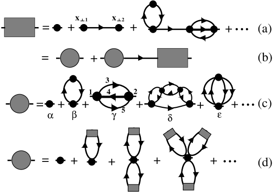
FIG. 1.: Diagrammatic expansion in $t_{\perp}$ of the single-particle Green’s function ${\cal G}$ (gray box). A directed line connecting two chains ${x_{\perp}}_{1}$ and ${x_{\perp}}_{2}$ gives a contribution $\hbox{$t_{\perp}$}({x_{\perp}}_{1}-{x_{\perp}}_{2})$, or $\hbox{$t_{\perp}$}({k_{\perp}})$ in momentum space [32]. A dot with $n$ entering and $n$ leaving lines contributes a factor ${\cal G}^{0}_{c}$ ($n$-particle cumulant of the uncoupled LL, see Sec. III). (a) Example of single-particle irreducible and reducible contributions to ${\cal G}$. (b) Dyson’s equation for ${\cal G}$ in terms of the inverse-self-energy $\Gamma$ (gray disk). (c) Example of diagrams contributing to $\Gamma$. (d) Self-consistent diagrams contributing to $\Gamma$ in the $D\to\infty$ limit. The self consistency is due to the presence of the full ${\cal G}$ in the internal lines of the loop.

Boies et al. used a functional–integral method to obtain an expansion in $t_{\perp}$ about the LL [13]. Although their formulation allows, in principle, for an expansion to any order in $t_{\perp}$ , in practice one can just get the first few orders. Our method provides a systematic diagrammatic formulation of this expansion to any order. The advantage of a diagrammatic formulation is that one can choose a class of diagrams to sum over, according to some physical guidance, without being restricted to the few lowest–order terms. This is particularly important for the model at study, since, as discussed in the Introduction, each power of $t_{\perp}$ in the perturbation carries a term $\hbox{${\cal E}_{\parallel}$}^{\alpha-1}$, which diverges precisely in the important region. Thus, one cannot reliably restrict to a finite number of diagrams.

Some diagrams contributing to the expansion of the Green’s function ${\cal G}$ (gray box) are shown in Fig. 1a. As in conventional perturbation theory, one can consider the function $\Gamma$ obtained by the sum of irreducible diagrams, i. e., the ones which cannot be separated by cutting a single line (see Fig. 1c). One then obtains a Dyson-like equation for ${\cal G}$ as a function of $\Gamma$ (Fig. 1b) of the form [32]

$${\cal G}({\bf k})=\left[\Gamma({\bf k})^{-1}-\hbox{$t_{\perp}$}({k_{\perp}})\right]^{-1}\;.$$ (2)

Notice that $\Gamma^{-1}$, and not $\Gamma$, appears in the inverse Green’s function contrary to standard perturbation theory. For this reason, we call $\Gamma$ inverse self energy.

The lowest–order approximation for $\Gamma$ (the “dot”: $\alpha$ in Fig. 1) corresponds to taking $\Gamma={\cal G}^{0}$, the Green’s function of the isolated LL. This gives for the total Green’s function Eq. (2) [32]

$${\cal G}({\bf k})=\left[{\cal G}^{0}({\bf k})^{-1}-\hbox{$t_{\perp}$}\hbox{$c_{\perp}$}\right]^{-1}\;.$$ (3)

This expression is a generalization of the Hubbard I approximation for the case of an expansion about the LL. Eq. (3) has been first obtained by Wen via a different procedure [37], and reobtained by Boies et al. [13] within a functional–integral method. This approximation, which we will refer to as “LO ”, is also called “single–dot”, “RPA”, “Wen’s”, or “Hubbard I” in other papers. For $\alpha<1$, the effect of the interchain kinetic energy $t_{\perp}$$c_{\perp}$ is to change the branch-cut singularity into a true quasiparticle pole (cf. Ref. [38]) for all $k$ points close to the FS, except for those ${k_{\perp}}$ points for which $\hbox{$c_{\perp}$}=0$ (for example, for $D=2$ these are ${k_{\perp}}=\pm\pi/2$). In particular, the positions of the poles for $\omega=0$ identify the new FS, which acquires a dispersion of the form ${k_{\parallel}}_{F}({k_{\perp}})\propto(\hbox{$t_{\perp}$}\hbox{$c_{\perp}$})^{1/(1-\alpha)}$, i. e. it is reduced with respect to the noninteracting case, where one would have ${k_{\parallel}}_{F}({k_{\perp}})\propto\hbox{$t_{\perp}$}\hbox{$c_{\perp}$}$, but not completely suppressed[10]. For the sake of completeness, we discuss the main results of this approximation in Sec. B.

Since the branch cut are shifted into poles, this approximation gives a FL along the whole FS except close to the $\hbox{$c_{\perp}$}=0$ region. This can be also seen from the quasiparticle weight $Z$, plotted in Fig.4 (dashed line), which vanishes for $\hbox{$c_{\perp}$}=0$. For this reason, the quasiparticle peak is quite broad in this region, as can be seen from Fig.6. However, as discussed above, this result, being restricted to lowest order is uncontrolled in the region $\hbox{${\cal E}_{\parallel}$}\ll\hbox{$t_{eff}$}$ and one should sum an infinite series of diagrams in order to get reliable results. Since it is not possible to sum all diagrams in the expansion, we want to select a workable subset of diagrams according to some physical limit in order to avoid an arbitrary choice. Specifically, we consider the series given by the diagrams indicated in Fig. 1d, corresponding to the large-dimension limit ($D\to\infty$). The $D\to\infty$ procedure adopted here is different from the standard dynamical mean-field theory  [39], since our system is strongly anisotropic, as the hopping in one (in the $\parallel$) direction is not rescaled by the usual $1/{\sqrt{D^{\prime}}}$ factor and is much larger than in the other $D-1$ ($\perp$) directions [32]. In analogy to the standard $D\to\infty$ method [39], where one has a single impurity embedded in a self–consistent medium, our $D\to\infty$ system represents a 1-D chain embedded in an effective self-consistent medium. As a consequence, the self-energy is local with respect to the $\perp$ coordinates but has a nontrivial dependence on the $\parallel$ ones [40]. We believe that this is the correct starting point to study the crossover problem, since, in this way, one treats the one-dimensional problem exactly and includes the coupling to the other chains by an effective dynamical mean field.

Even summing all the $D=\infty$ diagrams is an impossible task. Nevertheless, since we are interested in low-energy properties, we can restrict to the leading singularities in each diagram. It turns out convenient to rewrite the power expansion in terms of the dressed hopping ${\cal T}_{\perp}$ (indicated by a dashed line in Fig. 2). This is very similar to the skeleton expansion in conventional perturbation theory, where self-energy insertions are removed. The advantage is that the scaling behavior of the effective hopping (cf. Eq. (C13)) exactly cancels the power-law divergences of the diagrams, and each term of the perturbation acquires the same scaling as a function of the energy, and only logarithmic divergences are left.

The procedure of summing just the leading logarithmic divergences is similar in spirit to the sum of the leading divergences in the parquet series, which was introduced by the Russian [41] and by the French [42] school in order to study the instabilities of various one- and higher-dimensional electron systems. This method is equivalent to the one-loop renormalization-group ($g$-ology) approach[43], and it actually gives a rigorous background, as well as a systematic formulation for the extension of the $g$-ology method to higher dimensions. In our case, this corresponds to considering the quantity $l=\alpha\log(\hbox{$t_{eff}$}/\hbox{${\cal E}_{\parallel}$})$ to be of order one, and thus taking all orders in $l$, while considering $\alpha$ small.

Similarly, in the parquet summation, or $g$-ology[43], the small parameter is the bare interaction vertex $g_{0}$ and one sums all powers of $g_{0}\log\frac{E_{F}}{\omega}$, $\omega$ being the characteristic energy scale. The sum of this series gives the renormalized interaction vertex $g(\omega/E_{F})$ which thus acquires an energy dependence. Within the renormalization–group picture, the energy-dependent interaction vertex is interpreted as an effective interaction acting on an effective low-energy subspace, i. e., on a subspace in which high-energy modes are integrated out. Whenever the interaction vertex scales to zero, this signals that the effective low-energy theory describes non-interacting electrons, i. e., the theory is asymptotically (infrared) free. As a consequence, the exponents of correlations functions are mean-field like and, in the case of fermions, the system is a Fermi liquid. On the other hand, when a vertex diverges, no controlled prediction can be made about the low-energy behavior of the system, since the perturbative approach breaks down for sufficiently low energies, even when $g_{0}$ is small. In this case, the divergent vertex signals an instability towards some kind of broken-symmetry state.

In our case, the role of the interaction vertex is played by the anomalous exponent $\alpha$. The bare $\alpha$ is the correlation exponent of the uncoupled set of Luttinger liquids. Switching on the interliquid hopping $t_{\perp}$ produces a renormalization of the exponent. This renormalized exponent is obtained by looking at the low-energy behavior of the self-energy in the coupled-chains system. Similarly to the $g$-ology case, our result, obtained by summing the leading logarithmic divergences, is thus controlled if (i) the starting (bare) value of $\alpha$ is not too large and (ii) $\alpha$ scales to zero for low energies. The first (i) requirement is easy to fulfill, since for most interesting systems $\alpha$ is quite small For example, for the Hubbard model $\alpha\leq\frac{1}{8}$, where the equal sign holds for an infinite value of the on-site interaction $U$. Larger values of $\alpha$ are obtained by increasing the range of the interaction [44]. This is another reason why our approach is more convenient than a weak-coupling expansion in $U$: while our calculation makes sense also for very large (bare) $U$, for which $\alpha$ is still small, the weak-coupling renormalization group is not justified for $U$ larger than the bandwidth. An estimate of the maximum value $\alpha_{c}$ of $\alpha$, for which our calculation is justified is given in Sec. V. The second (ii) requirement can be only checked a posteriori. The main result of this paper is that indeed point (ii) turns out to be satisfied, as $\alpha$ scales to zero for energies smaller than $t_{eff}$ . Thus, our procedure of restricting to the leading logarithmic divergences is controlled, unless one starts from a model with a too large value of $\alpha$.

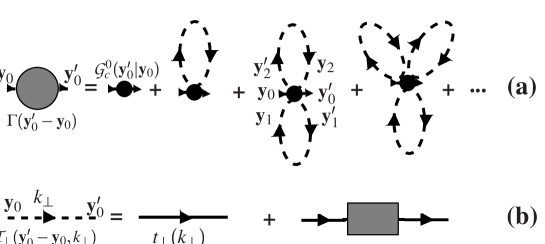
FIG. 2.: (a) Diagrams contributing to the inverse-self-energy $\Gamma$ in the $D=\infty$ limit within an expansion in the dressed hopping ${\cal T}_{\perp}$ (dashed line). (b) Dressed hopping and its diagrammatic expression in terms of the bare hopping $t_{\perp}$ (full line) and the Green’s function. Other conventions are as in Fig. 1.

III Anisotropic $D\to\infty$ method

In this section, we carry out the sum of the $D\to\infty$ diagrams for the inverse-self-energy. In the $D\to\infty$ limit, the inverse-self-energy $\Gamma({\bf x}_{0})$ is $\perp$-local [40], and is obtained as the sum of the loop diagrams in Fig. 2a (equivalent to the ones of Fig. 1d) as

$$\Gamma({\bf x}_{0})={\cal G}^{0}_{c}({\bf x}_{0}|0)+\sum_{m=1}^{\infty}\frac{(-1)^{m}}{m!}\int\Bigl{[}\prod_{k=1}^{m}d^{2}{\bf y}_{k}\ d^{2}{\bf x}_{k}\ \hbox{${\cal T}_{\perp}$}(-{\bf x}_{k},0)\Bigr{]}\,{\cal G}^{0}_{c}({\bf y}_{0}+{\bf x}_{0},\cdots,{\bf y}_{m}+{\bf x}_{m}|{\bf y}_{0},\cdots,{\bf y}_{m})\;,$$ (4)

$$={\cal G}^{0}_{c}({\bf x}_{0}|0)+\sum_{m=1}^{\infty}(-1)^{m}\int_{1\downarrow m}\Bigl{[}\prod_{k=1}^{m}d^{2}{\bf y}_{k}\ d^{2}{\bf x}_{k}\ \hbox{${\cal T}_{\perp}$}(-{\bf x}_{k},0)\Bigr{]}\,{\cal G}^{0}_{c}({\bf y}_{0}+{\bf x}_{0},\cdots,{\bf y}_{m}+{\bf x}_{m}|{\bf y}_{0},\cdots,{\bf y}_{m})\;,$$ (5)

where in the last line we have exploited the symmetry for exchange of the coordinates $1,\cdots,m$ and restricted the integration to the region $|{\bf x}_{1}|>|{\bf x}_{2}|>\cdots>|{\bf x}_{m}|$ indicated by “$1\downarrow m$”. The corresponding factor $m!$ is then canceled by the symmetry factor $1/m!$ of the diagram. In Eq. (4), ${\cal G}^{0}_{c}({\bf y}_{0}^{\prime}\cdots{\bf y}_{m}^{\prime}|{\bf y}_{0}\cdots{\bf x}_{m})$ is the $m+1$-particle cumulant of the uncoupled LL, i. e. the connected part of the $m+1$-particle Green’s function ${\cal G}^{0}_{c}({\bf y}_{0}^{\prime}\cdots{\bf y}_{m}^{\prime}|{\bf y}_{0}\cdots{\bf x}_{m})$ defined in Eq. (A13) (see also Eq. (D36) for the definition of cumulants in terms of Green’s functions). In particular, for $m=0$ the single–particle cumulant ${\cal G}^{0}_{c}$ coincides with the Green’s function ${\cal G}^{0}$, as there are no disconnected parts. Moreover, $\hbox{${\cal T}_{\perp}$}({\bf x},x_{\perp}=0)$ is the dressed hopping written in real space, which is calculated in Sec. C.

We are interested in the dominant low-energy behavior ($\hbox{${\cal E}_{\parallel}$}\ll\hbox{$t_{eff}$}$ corresponding to $|{\bf x}_{0}|\hbox{$t_{eff}$}\gg 1$) of correlation functions and thus we can restrict to the leading logarithmic divergences in the loop integrals ( Eq. (4)), as discussed in Sec. II. Let us estimate this leading contribution. If, as a first step, one neglects the self-consistency of the Green’s function and dresses the hopping ${\cal T}_{\perp}$ with the bare Green’s function only ( Eq. (C13)), one can see that the leading contribution of a $m$-loop term in Eq. (4) has the form ${\cal G}^{0}_{c}({\bf x}_{0}|0)\times(\alpha\log|{\bf x}_{0}|\hbox{$t_{eff}$})^{2m}$. Indeed, one “$\alpha\log$” term arises from each integration of the “center of mass” coordinates ${\bf y}_{k}$ (cf. Sec. D), another “$\alpha$” from each ${\cal T}_{\perp}$, due to its real-space structure (cf. Eq. (C13)), and a “$\log$” comes out for each integration of the “relative” coordinates ( Eq. (15)).

Even summing up “just” the leading logarithmic divergences of the integrals in Eq. (4) is a tough task. To do this we proceed in several steps. First, consider that some integration regions in Eq. (4) can be left out, as they don’t contribute to the leading logarithmic divergences. Specifically, in addition to the region $|{\bf x}_{1}|>|{\bf x}_{2}|>\cdots>|{\bf x}_{m}|$ (called $1\downarrow m$), to which we restrict by symmetry, we can further restrict to the region[45] $|{\bf x}_{0}|>|{\bf x}_{1}|$, and $|{\bf x}_{p}|<min(|{\bf y}_{q}-{\bf y}_{r}|,|{\bf y}_{q}^{\prime}-{\bf y}_{r}|,|{\bf y}_{q}^{\prime}-{\bf y}_{r}^{\prime}|)$ for each $p\geq q,r$ (of course, $q\not=r$), and ${\bf y}_{q}^{\prime}$ is defined as ${\bf y}_{q}+{\bf x}_{q}$. The fact that the leading logarithmic contributions only come from this integration region, which we will call “$0\Downarrow m$”, is proven in Sec. E.

For convenience, we introduce the “restricted renormalized cumulants” (RRC) [46], defined only in the region “$0\Downarrow m$” as

$${\cal G}_{c}({\bf y}_{0}+{\bf x}_{0},\cdots,{\bf y}_{m}+{\bf x}_{m}|{\bf y}_{0},\cdots,{\bf y}_{m})$$ (6)

$$\equiv{\cal G}^{0}_{c}({\bf y}_{0}+{\bf x}_{0},\cdots,{\bf y}_{m}+{\bf x}_{m}|{\bf y}_{0},\cdots,{\bf y}_{m})$$ (7)

$$-\int_{0\Downarrow m+1}d^{2}{\bf x}_{m+1}\ d^{2}{\bf y}_{m+1}\ \hbox{${\cal T}_{\perp}$}(-{\bf x}_{m+1},0)$$ (8)

$$\times{\cal G}_{c}({\bf y}_{0}+{\bf x}_{0},\cdots,{\bf y}_{m+1}+{\bf x}_{m+1}|{\bf y}_{0},\cdots,{\bf y}_{m+1})\;.$$ (9)

Comparing Eq. (4) and Eq. (6), it is straightforward to verify that $\Gamma({\bf x}_{0})$. is given by the single-particle RRC, ${\cal G}_{c}({\bf x}_{0}|0)$.

We thus proceed by evaluating the integrals in Eq. (6). An important point, which we will show below, is that, at the leading logarithmic order, the $m+1$-particle cumulant is renormalized by a multiplicative factor, which depends on the absolute values of the relative coordinates $|{\bf x}_{i}|$ only. More precisely, the RRC can be written as

$${\cal G}_{c}({\bf y}_{0}+{\bf x}_{0},\cdots,{\bf y}_{m}+{\bf x}_{m}|{\bf y}_{0},\cdots,{\bf y}_{m})$$ (11)

$$={\cal F}_{m}(l_{0},\cdots,l_{m})\ {\cal G}^{0}_{c}({\bf y}_{0}+{\bf x}_{0},\cdots,{\bf y}_{m}+{\bf x}_{m}|{\bf y}_{0},\cdots,{\bf y}_{m})$$

where the ${\cal F}_{m}$ is the renormalization factor, which we have written in terms of the logarithmic variables $l_{i}\equiv\alpha\log(|{\bf x}_{i}|\hbox{$t_{eff}$})$. We can thus first carry out the integration over the “center-of-mass” coordinate ${\bf y}_{m+1}$ in Eq. (6) by simply considering the effect on the bare cumulant, as the renormalization factor does not depend on ${\bf y}_{m+1}$. This integral is quite involved, but its leading logarithmic contribution can be calculated analytically. This is carried out in Sec. D, where one obtains [32]

$$\int\limits_{0\Downarrow m+1}d^{2}{\bf y}_{m+1}\;{\cal G}^{0}_{c}({\bf y}_{0}+{\bf x}_{0},\cdots,{\bf y}_{m+1}+{\bf x}_{m+1}|{\bf y}_{0},\cdots,{\bf y}_{m+1})$$ (12)

$$=2\pi\ {\cal G}^{0}_{c}({\bf y}_{0}+{\bf x}_{0},\cdots,{\bf y}_{m}+{\bf x}_{m}|{\bf y}_{0},\cdots,{\bf y}_{m})$$ (13)

$$\times|{\bf x}_{m+1}|^{2}\ {\cal G}^{0}_{c}({\bf x}_{m+1}|0)\ \sum_{j=1}^{m}\alpha\ \left(\log|{\bf x}_{j}|-\log|{\bf x}_{m+1}|\right)\ \left(\delta_{r_{j},r_{m+1}}+\frac{1}{S}\ \delta_{r_{j},-r_{m+1}}\right)\;.$$ (14)

After carrying out the integral over ${\bf y}_{m+1}$ we carry out the integration over the “relative” coordinate ${\bf x}_{m+1}$, which includes a sum over $r$ and $\sigma$ [32]. Inserting the form Eq. (11) and the result Eq. (12) into Eq. (6), and dividing both sides of the equation by ${\cal G}^{0}_{c}({\bf y}_{0}+{\bf x}_{0},\cdots,{\bf y}_{m}+{\bf x}_{m}|{\bf y}_{0},\cdots,{\bf y}_{m})$, one obtains

$${\cal F}_{m}(l_{0},\cdots,l_{m})=1-2\ \pi\ \int\limits_{\hbox{$t_{eff}$}^{-1}<|{\bf x}_{m+1}|<|{\bf x}_{m}|}d^{2}{\bf x}_{m+1}\ \hbox{${\cal T}_{\perp}$}(-{\bf x}_{m+1},0)\ |{\bf x}_{m+1}|^{2}\ {\cal G}^{0}_{c}({\bf x}_{m+1}|0)\$$ (15)

$$\times{\cal F}_{m+1}(l_{0},\cdots,l_{m},l_{m+1})\ \sum_{j=1}^{m}\left(l_{j}-l_{m+1}\right)\ \left(\delta_{r_{j},r_{m+1}}+\frac{1}{S}\ \delta_{r_{j},-r_{m+1}}\right)\;,$$ (16)

where the lower limit of integration for $|{\bf x}_{m+1}|$ is due to the fact that ${\cal T}_{\perp}$ changes its behavior in the region $E_{F}^{-1}<|{\bf x}_{m+1}|<\hbox{$t_{eff}$}^{-1}$ (Ref. [47]) , and, thus, there is no logarithmic contribution here, and the upper one is due to the restriction $0\Downarrow m+1$ in Eq. (6). Inserting the asymptotic expression for the dressed hopping Eq. (C22) in Eq. (15), one can carry out the integration over ${\bf x}_{m+1}$ in circular coordinates, and obtain the recursive self-consistent equation for ${\cal F}_{m}$

$${\cal F}_{m}(l_{0},\cdots,l_{m})=1+2(1+S)\ \int_{0}^{l_{m}}dl_{m+1}\ \sum_{j=0}^{m}\ (l_{j}-l_{m+1})$$ (17)

$$\times\ {\cal F}_{m+1}(l_{0},\cdots,l_{m+1})\ \left[\bar{\cal F}_{0}(l_{m+1})+\bar{\cal F}_{0}^{\prime}(l_{m+1})\right]\;.$$ (18)

From Eq. (17), it is obvious that ${\cal F}_{m}$ depends on just two variables, namely $l\equiv l_{0}+\cdots+l_{m-1}$, and $l_{m}$. With this redefinition, and renaming the integration variable $l_{m+1}$ to $l^{\prime}$, Eq. (17) can be reduced to

$${\cal F}_{m}(l,l_{m})=1+2(1+S)\ \int_{0}^{l_{m}}dl^{\prime}\ [l+l_{m}-(m+1)\ l^{\prime}]\ {\cal F}_{m+1}(l+l_{m},l^{\prime})\ \left[\bar{\cal F}_{0}(l^{\prime})+\bar{\cal F}_{0}^{\prime}(l^{\prime})\right]\;.$$ (19)

Eq. (19) is a self-consistent equation, since $\bar{\cal F}_{0}=1/{\cal F}_{m=0}$ [ Eq. (C18)], which depends on the ${\cal F}_{m}$, to insert on the r.h.s.. We have not been able to find an analytic solution to Eq. (19). However, by expanding in powers of of the variables $l_{i}$ one can write a recursive equation for the coefficients of the expansion of the functions ${\cal F}_{m}$ up to a rather high order with a moderate numerical effort. This procedure is described in detail in Sec. F.

We have evaluated the coefficients of ${\cal F}_{0}$ up to the $42^{th}$ order in $l$. A Mathematica program has allowed us to evaluate these coefficients in a rational form, which is particularly recommended for a Padé analysis. A straight summation of the series is not recommended, since its convergence radius seems to be rather small (of the order unity), while we need the asymptotic behavior for large $l$. Nevertheless $l=\alpha\log(|{\bf x}|\hbox{$t_{eff}$})$ is restricted to the neighborhood of the real positive axis, and a Padé analysis shows that the poles are either away on the complex plane or on the negative real axis. A Padé analysis is thus the most appropriate procedure in order to determine the large-$l$ behavior of the function ${\cal F}_{0}(l)$, which also gives the asymptotic behavior of the inverse self-energy $\Gamma(x)$. The results will be presented and discussed in Sec. IV.

IV Results and discussion

As shown in Sec. F, the solution of Eq. (19) gives ${\cal F}_{0}(l)\sim e^{cl}$ for large $l$, where the exponent $c$ turns out to be essentially equal to $1$ (within about $10^{-4}$ of accuracy) in both cases with and without spin. Introducing this result and Eq. (A14) in the expression for the inverse-self-energy ( Eq. (11) with $m=0$) yields

$$\Gamma({\bf x})={\cal G}^{0}({\bf x}|0)\ {\cal F}_{0}(\alpha\log(|{\bf x}|\hbox{$t_{eff}$}))\to{\cal G}^{0}({\bf x}|0)\ (|{\bf x}|\ \hbox{$t_{eff}$})^{\alpha}\propto\hbox{$t_{eff}$}^{\alpha}/|{\bf x}|\;,$$ (20)

i. e. the anomalous exponent $\alpha$ exactly cancels out in the asymptotic behavior of $\Gamma$!. The same thing happens in momentum space. From Eq. (C17) one notices that the (asymptotic behavior of the) renormalization function is the same in momentum space, provided one replaces $|{\bf x}|$ with $1/|{\bf k}|$. Thus, for low energies we obtain for the right-moving component ($r=+1$)

$$\Gamma({\bf k})\to{\cal G}^{0}({\bf k})\ \hbox{$t_{eff}$}^{\alpha}\ |{\bf k}|^{-\alpha}\propto\hbox{$t_{eff}$}^{\alpha}\ (i\omega-{k_{\parallel}})^{-1}\;,$$ (21)

where we have used Eq. (C8).

The Green’s function of the coupled system is given by the Dyson equation Eq. (2). Taking the result Eq. (21), one can readily notice that the Green’s function now has poles at $i\omega-{k_{\parallel}}\propto\hbox{$t_{eff}$}^{\alpha}\hbox{$t_{\perp}$}({k_{\perp}})$, i. e. even for $\hbox{$c_{\perp}$}=0$, in contrast to the LO result, where a branch cut was present. In particular, at the FS ($i\omega\to 0+i0^{+}$) and for $\hbox{$c_{\perp}$}=0$, our result becomes asymptotically exact, as $|{\bf k}|$ vanishes at the pole.

Let us look at the FS more precisely. This is the curve ${k_{\parallel}}_{F}(\hbox{$c_{\perp}$})$ parametrized by the Fermi momentum as a function of the $\perp$ momenta, and is determined by the solution of the equation $\Gamma({k_{\parallel}}_{F}(\hbox{$c_{\perp}$}),i\omega=0+i0^{+})^{-1}=\hbox{$t_{\perp}$}\hbox{$c_{\perp}$}$. Obviously, Eq. (21) gives ${k_{\parallel}}_{F}(\hbox{$c_{\perp}$}=0)=0$. In Fig. 3 we plot the FS curve for other values of $c_{\perp}$, and $\alpha=1/4$ in the case of particles with spin. We compare our result (full line) with the LO result (dashed line). For small $c_{\perp}$ , our result gives a regular behavior ${k_{\parallel}}_{F}(\hbox{$c_{\perp}$})\propto\hbox{$t_{eff}$}\ \hbox{$c_{\perp}$}$ in contrast to the lowest-order result, which gives a flattening of the FS at $\hbox{$c_{\perp}$}=0$, due to the behavior ${k_{\parallel}}_{F}(\hbox{$c_{\perp}$})\propto\hbox{$t_{eff}$}\ \hbox{$c_{\perp}$}^{1/(1-\alpha)}$.

The quasiparticle weight $Z(\hbox{$c_{\perp}$})$ at the FS is given by the inverse of the coefficient of the linear term in $\omega$ in the inverse Green’s function, more precisely, $Z(\hbox{$c_{\perp}$})^{-1}=\frac{d}{di\omega}1/{\cal G}({k_{\parallel}}_{F}(\hbox{$c_{\perp}$}),i\omega)_{i\omega\to 0+i0^{+}}$. We have plotted $Z$ as a function of $c_{\perp}$ for the case with spin in Fig. 4, again compared with the LO approximation. Moreover, in order to show the importance of summing the infinite series of diagrams, we have included the result obtained by truncating the $D\to\infty$ series (Fig. 2a) at the first loop, by still taking the self–consistently dressed hopping as internal line. For small $c_{\perp}$ , the lowest-order result (dashed line) gives a $Z$ vanishing as $Z(\hbox{$c_{\perp}$})\propto(\hbox{$t_{\perp}$}\hbox{$c_{\perp}$})^{\alpha/(1-\alpha)}$, thus yielding poorly defined quasiparticles around $\hbox{$c_{\perp}$}=0$. Inclusion of the first loop (dotted line) gives a vanishing Z too. Therefore, self consistency is not enough to restore the FL behavior. Our result, instead, yields a finite $Z$ for $\hbox{$c_{\perp}$}\to 0$, as can be seen from the figure (solid line). The correct FL behavior is thus recovered on the whole FS, including the regions $\hbox{$c_{\perp}$}=0$.

FIG. 3.: Fermi-surface dispersion ${k_{\parallel}}_{F}$ as a function of the off-chain kinetic energy $c_{\perp}$ (in units of $t_{\perp}$ ) for the coupled spinful Luttinger liquids [ Eq. (1)] with bare LL exponent $\alpha=1/4$. Our $D\to\infty$ result (solid line) is compared with the LO approximation Eq. (3) (dashed).

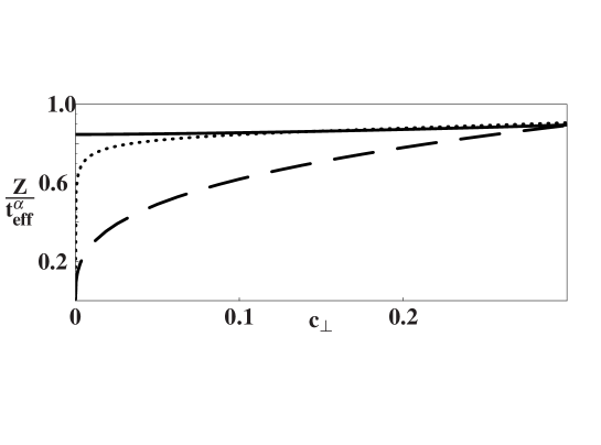
FIG. 4.: Quasiparticle weight Z as a function of the off-chain kinetic energy $c_{\perp}$ with the same conventions as in Fig. 3 . In addition, we show the result (dotted line) obtained by partially improving on the LO approximation, i. e., by including the first self-consistent loop for the inverse self-energy of Fig. 1d.

These results can be more concretely seen in the spectral function for small $c_{\perp}$ [48]. This is plotted in Fig. 5 for different $c_{\perp}$, and for ${k_{\parallel}}=0$. The figure shows a well–defined dispersive quasiparticle peak, which becomes sharper by approaching the FS, as should be the case for a FL. The dispersion as a function of $c_{\perp}$ is a clear indication of higher–dimensional coherence. For comparison, in Fig. 6, we have shown the LO result. As one can see, the peak is dispersive too, but much broader and lower (notice the different scale). Moreover, a closer inspection shows that the quasiparticle weight decreases by approaching the FS, which is consistent with what we have shown in Fig. 4.

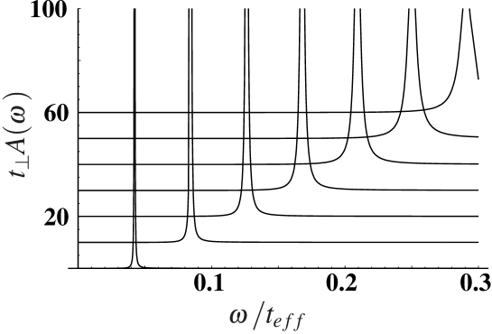
FIG. 5.: Spectral function $A(\omega)$ of the coupled spinful Luttinger liquids for different values of $c_{\perp}$, ${k_{\parallel}}=0$, and $\alpha=1/4$ from our $D\to\infty$ result. For the sake of clarity, the different curves are shifted vertically by steps of $10$. They correspond to $\hbox{$c_{\perp}$}=0.05,0.1,0.15,0.2,0.25,0.3,0.35$, from bottom to top. Notice the sharpening of the peaks upon approaching the FS at $\hbox{$c_{\perp}$}\to 0$.

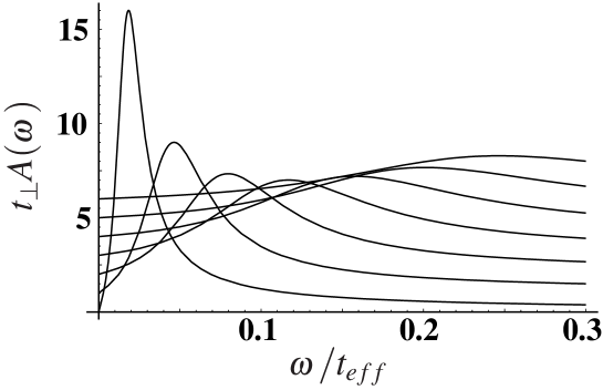
FIG. 6.: Spectral function $A(\omega)$ from the LO approximation for the same parameters as in Fig. 5, except that the curves are shifted by $1$. The peaks sharpen upon approaching the FS, but the quasiparticle weight vanishes.

We want to study the spectral function even for ${k_{\parallel}}\not=0$. To understand what happens, let us first look at the spectral function for the LM [3, 4] (without spin-charge separation), which we plot in Fig. 7 for ${k_{\parallel}}=0.2$. From the figure, one can readily recognize the two nonanalicities at $\omega\pm{k_{\parallel}}$. For $\omega\searrow+{k_{\parallel}}$ one has in fact a divergence like $(\omega-{k_{\parallel}})^{\alpha/2-1}$, while for $\omega\nearrow-{k_{\parallel}}$ the spectral function vanishes as $({k_{\parallel}}+\omega)^{\alpha/2}$. The power–law divergence instead of a pole at $\omega={k_{\parallel}}$ is due to the fact that the point, $\omega={k_{\parallel}}$, where the inverse Green’s function, $1/{{\cal G}^{0}}$, of the LL vanishes, is not a simple zero but a branch cut. Between $\pm{k_{\parallel}}$ the spectral function of the LM is identically zero, as the Green’s function has neither cuts nor poles here. At ${k_{\parallel}}=0$ the two nonanalicities merge in a single power-law divergence $\omega^{\alpha-1}$.

FIG. 7.: Spectral function of the isolated Luttinger model (with equal charge and spin velocities) for $\alpha=1/4$ and ${k_{\parallel}}=0.2$ [3, 4].

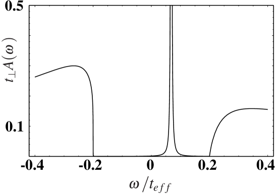
FIG. 8.: Spectral function within the LO approximation for the coupled spinful Luttinger liquids with $\alpha=1/4$, ${k_{\parallel}}=0.2$, and $\hbox{$c_{\perp}$}=-0.2$. In order to make the quasiparticle delta function visible, we have added a small imaginary part $\sim 3.0\ 10^{-5}$. Due to the proximity of the singularity, the peak actually becomes broader.

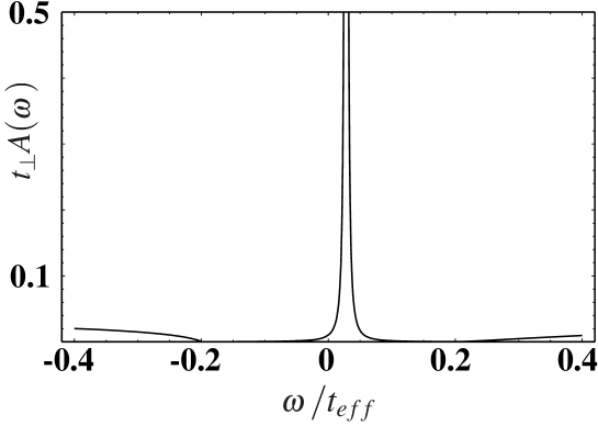
FIG. 9.: Spectral function for the $D\to\infty$ result with the same parameters as in Fig. 8. Notice the much larger transfer of spectral weight from the singularities to the quasiparticle pole.

Within the LO approximation, Eq. (3), the zero of $1/{{\cal G}}$ is shifted away from the branch cut. Thus, an isolated quasiparticle pole appears in the region $-{k_{\parallel}}<\omega<{k_{\parallel}}$ on the real axis. This pole is always present for any $\hbox{$c_{\perp}$}\not=0$ (see Sec. B). The pole removes spectral weight from the peak at $\omega={k_{\parallel}}$ which is now no longer a divergence.

In our $D\to\infty$ result, the situation is similar. However, Fig. 9 shows that in this case the two singularities at $\pm{k_{\parallel}}$ loose much more spectral weight in favor of the pole. This is another reason why the quasiparticle weight remains larger within our result, as shown in Figs. 4, and 5. For $\hbox{$c_{\perp}$}=0$ Eq. (3) does not have quasiparticle poles, while our result yields a pole with nonvanishing weight at the FS even in this case. The reason for that is due to the different behavior of the quasiparticle weight, as shown in Fig. 4, and by the fact that the scattering rate does not vanish fast enough for Eq. (3), while it vanishes faster than linearly within our result, as discussed in Ref. [11] (cf. Fig. 2c of that reference).

V Conclusions

In conclusion, we have studied the problem of the crossover from one to higher dimensions for fermionic systems, when Luttinger liquids are coupled by a small hopping $t_{\perp}$ . Specifically, we have concentrated on the region below the single–particle crossover temperature, $\hbox{${\cal E}_{\parallel}$}\ll\hbox{$t_{eff}$}$, which is the one relevant for the dimensional crossover. We have carried out an expansion in powers of $t_{\perp}$ , and summed the self–consistent series of diagrams (Fig. 1d) corresponding to the anisotropic $D\to\infty$ limit. Our result shows that the LL exponent $\alpha$ renormalizes to zero for energies smaller than the single-particle crossover temperature $t_{eff}$. The system thus flows to a FL fixed point with mean-field like exponents. This is seen, for example, in the self–energy, which now scales linearly as a function of frequency and momentum, in contrast to the LO approximation Eq. (3), where the self–energy still scales anomalously like $|{\bf k}|^{1-\alpha}$ . As a consequence, well defined quasiparticles are recovered along and in the neighborhood of the whole FS, in contrast to the result Eq. (3), where the spectrum is incoherent for small $c_{\perp}$ .

We have shown the importance of including an infinite series of diagrams, in order to give reliable results in the region $\hbox{${\cal E}_{\parallel}$}\ll\hbox{$t_{eff}$}$. Even introducing the first loop of the diagrammatic expansion (in Fig. 1d) does not give the correct result, as shown in Fig. 4. This shows that not even a self–consistent calculation is sufficient. This is the reason why previous theoretical results, restricted to lowest orders, are still contradictory about the nature of the ground state in this energy region.

These results have been obtained for the case of equal spin and charge velocities. In fact, we believe that the scaling behavior of the anomalous exponent $\alpha$ found here is universal and should not be affected by the inclusion of spin–charge separation. Nevertheless, an extension of the present calculation to the case of LLs with different velocities could be interesting, first, in order to check this fact, and second, in order to verify whether spin–charge separation scales as well to zero in higher dimension like $\alpha$, or not.

The imaginary part of the self energy, $-Im\ \Gamma^{-1}$, needed to evaluate the spectral functions in Figs. 5 and 9 has been determined by analytic continuation of the asymptotic form Eq. (21) [48]. However, one should mention that our calculation, restricted to the leading divergences, yields reliable results for $Im\Gamma^{-1}$ at small values of $\omega$ and ${k_{\parallel}}$ only. On the FS and for large $c_{\perp}$ , ${k_{\parallel}}$ is large too. Thus, for large $c_{\perp}$ , we cannot state with certainty whether corrections to $Im\Gamma^{-1}$ beyond the leading divergences vanish fast enough upon approaching the FS or not. Arguments similar to the one of ordinary perturbation theory[49] cannot be extended to the present case, due to the momentum dependence of the vertices in the $t_{\perp}$ expansion. A hint can be possibly obtained by explicitly evaluating numerically the first few loops in Fig. 1d, without restricting to the leading divergences.

In principle, we cannot say whether our result is valid also for the physical cases of finite dimensions, and, in particular for $D=2$ or $D=3$. However, as we have shown in Sec. C 2, the non-$\perp$-local dressed hopping $\hbox{${\cal T}_{\perp}$}({\bf x},x_{\perp}\not=0)$ vanishes faster than the $\perp$-local one $\hbox{${\cal T}_{\perp}$}({\bf x},0)$ for large $|{\bf x}|$. Non $\perp$-local contributions are thus irrelevant and one may try to extend the present result to finite dimensions. However, there are still $\perp$-local diagrams of order $1/D$, (for example, if one takes the diagram $\gamma$ of Fig. 1 and replaces all internal line with a local ${\cal T}_{\perp}$), which may spoil this result. It might be interesting to consider an expansion about the present $D=\infty$ result, and consider the irrelevance or relevance of such diagrams, and give predictions about a possible critical dimension $D_{c}$, above which the results of this paper hold. For example, this could be done in order to study the critical behavior in the neighborhood of the transition to the two–particle regime at $\alpha=\alpha_{2p}$[10],where $\alpha_{sp}\sim 0.41$ ($0.62$) for spinless (spinful) electrons.

In Sec. II, we have already discussed that our “renormalization–group–like” result holds for $\alpha$ smaller than a certain $\alpha_{c}$. Although we cannot determine $\alpha_{c}$ exactly within our approach, we can estimate it, e. g., by the value of $\alpha$ for which the spectral function becomes negative in some regions. This criterion gives $\alpha_{c}\approx 0.50$ for the spinless and $\alpha_{c}\approx 0.33$ for the spinful case.

Another question is the contribution of the shifted poles $|{\bf k}|,\hbox{$c_{\perp}$}\not=0$, which turn out to be irrelevant in the present case (cf. Sec. C). However, these poles may give important contributions in lower dimensions. Indeed, these poles are the one giving rise, in some conditions, to the well known nesting or superconducting instabilities at selected regions of the FS.

The author thanks W. Hanke for useful discussions. Partial support by the BMBF (05SB8WWA1) is acknowledged.

A Many–particle correlation functions of the Luttinger liquid

For the sake of completeness, and in order to fix our notation, we give here the expressions for the $n$–particle Green’s functions of the LM in real space. To our knowledge, their explicit expression, although known, has not been reported anywhere else. In Sec. A 1, we discuss the scaling behavior of the diagrams in the $t_{\perp}$ expansion.

A generic $\perp$-local $n$-particle Green’s function is defined as [32]

$${\cal G}^{d_{1}\cdots d_{2n}}({\bf x}_{1},\cdots,{\bf x}_{2n})\equiv<T_{\tau}\psi^{d_{1}}({\bf x}_{1})\cdots\psi^{d_{2n}}({\bf x}_{2n})>\;,$$ (A1)

where $T_{\tau}$ is the imaginary-time ordering operator, $\psi^{d}({\bf x})$ destroys (for $d=-1$) or creates (for $d=+1$) a fermion at the point ${\bf x}$ (which includes $r$ and $\sigma$). In order to extract the $\hbox{$t_{\perp}$}=0$ cumulants ${\cal G}^{0}_{c}$ of the isolated LM, to be used in Eq. (4), we first need the (disconnected) Green’s functions ${\cal G}^{0}$. These can be written as

$${\cal G}^{0,d_{1}\cdots d_{2n}}({\bf x}_{1},\cdots,{\bf x}_{2n})=(2\pi a)^{-n}\eta_{r_{1}}\cdots\eta_{r_{2n}}\ \prod_{2n\geq i_{1}>i_{2}\geq 0}\left[P_{r_{i_{1}}r_{i_{2}}}({\bf x}_{i_{1}}-{\bf x}_{i_{2}})\right]^{-d_{i_{1}}d_{i_{2}}}\;.$$ (A2)

This holds whenever the particle- and momentum-conservation constraints $\sum_{i=1}^{2n}d_{i}=0$, and $\sum_{i=1}^{2n}d_{i}r_{i}=0$ are fulfilled, otherwise ${\cal G}^{0}=0$. Here, $a$ is a short-distance cutoff ($a\propto\frac{v_{F}}{E_{F}}$). The Klein factors $\eta_{r_{i}}$ obey anticommutation rules $\{\eta_{r},\eta_{r^{\prime}}\}=\delta_{r,r^{\prime}}$ and account for the fermionic anticommutations [50, 51]. From now on, we will set $a$ to unity, unless otherwise specified.

The functions $P$ in Eq. (A2) can be written as

$$P_{r_{1}r_{2}}({\bf x})={\cal R}({\bf x})^{-q(r_{1}\ r_{2},K_{\rho})}\ e^{i\frac{r_{1}+r_{2}}{2}\ \left(\frac{\pi}{2}-A({\bf x})\right)}\;,$$ (A3)

where the exponent $q(r_{1},r_{2},K_{\rho})$ is given by [32]

$$q(r,K_{\rho})= \left\{\matrix{\frac{1}{2}\ (rK_{\rho}+\frac{1}{K_{\rho}})&\hbox{ for }S=1\cr\frac{1}{4}\ [r(K_{\rho}+1)+\frac{1}{K_{\rho}}+1]&\hbox{ for }S=2}\right.$$ (A5)

$$=\left\{\matrix{1+\alpha&\hbox{ for }r=1\cr B&\hbox{ for }r=-1\cr}\right.\;,$$

where the LL exponent $\alpha$ is related to $K_{\rho}$ via

$$\frac{K_{\rho}+1/K_{\rho}-2}{2\ S}=\alpha\;,$$ (A6)

and

$$B\equiv\frac{1/K_{\rho}-K_{\rho}}{2S}\;.$$ (A7)

Here,

$${\cal R}({\bf x})\equiv\frac{\beta}{\pi a}\ \sqrt{\cosh^{2}\widetilde{{x_{\parallel}}}-\cos^{2}\widetilde{\tau}}\;,$$ (A8)

and

$$A({\bf x})\equiv\arg(\tanh\widetilde{{x_{\parallel}}}+i\tan\widetilde{\tau})\;,$$ (A9)

$\widetilde{x_{\parallel}}\equiv\frac{\pi{x_{\parallel}}}{\beta}$, $\widetilde{\tau}\equiv\frac{\pi\tau}{\beta}$. At zero temperature $T=\frac{1}{\beta}=0$, Eq. (A8) and Eq. (A9) become

$${\cal R}({\bf x})\to\sqrt{\frac{{x_{\parallel}}^{2}+\tau^{2}}{a^{2}}}=\frac{|{\bf x}|}{a}\;,$$ (A10)

and

$$e^{iA({\bf x})}\to e^{i\arg({x_{\parallel}}+i\tau)}=\frac{{x_{\parallel}}+i\tau}{|{\bf x}|}=\frac{{\bf x}\cdot{\bf v}}{|{\bf x}|}\;,$$ (A11)

where we have introduced the complex vector ${\bf v}=(1,i)$, allowing for a compact expression. These expressions are valid for $|{\bf x}|\gg a$ and need a short-distance cutoff for $|{\bf x}|\sim a$. The cutoff prescription for the LM amounts to replacing ${x_{\parallel}}^{2}+\tau^{2}$ with ${x_{\parallel}}^{2}+(|\tau|+a)^{2}$. However, it turns out convenient to adopt a “rotation symmetric” cutoff obtained by replacing ${x_{\parallel}}^{2}+\tau^{2}$ with ${x_{\parallel}}^{2}+\tau^{2}+a^{2}$, or by setting ${\cal R}({\bf x})=1$ for $|{\bf x}|<a$. The low-energy results, obviously, don’t depend on the specific choice of the short-distance cutoff. The advantage of setting equal spin and charge velocities is clear at this point. Without this assumption, the correlation functions would not be invariant under rotation in the $({x_{\parallel}},\tau)$ plane, which would have made the calculations more difficult.

In conformity with Ref. [11], we define

$${\cal G}^{0}({\bf y}_{0}^{\prime},\cdots,{\bf y}_{m}^{\prime}|{\bf y}_{0},\cdots,{\bf y}_{m}) \equiv{\cal G}^{0,1,-1,1,-1,\cdots}({\bf y}_{0},{\bf y}_{0}^{\prime},\cdots,{\bf y}_{m},{\bf y}_{m}^{\prime})$$ (A13)

$$=<T_{\tau}\psi^{{\dagger}}({\bf y}_{0})\psi({\bf y}_{0}^{\prime})\cdots\psi^{{\dagger}}({\bf y}_{m})\psi({\bf y}_{m}^{\prime})>_{\hbox{$t_{\perp}$}=0}\;,$$

and ${\cal G}_{c}^{0}({\bf y}_{0}^{\prime},\cdots,{\bf y}_{m}^{\prime}|{\bf y}_{0},\cdots,{\bf y}_{m})$ as the corresponding cumulant (or connected Green’s function) to be inserted in the diagrammatic expression Eq. (4).

As an example, we use Eq. (A2) to evaluate the single- and the two-particle Green’s functions (here, we indicate explicitly the indices $r$ as $1$ for $r=+1$ or $\bar{1}$ for $r=-1$). The single-particle Green’s function reads

$${\cal G}^{0}({\bf x}\,1|0\,1)=-\frac{i}{2\pi a}\ |{\bf x}|^{-1-\alpha}\ e^{-i\arg{\bf x}\cdot{\bf v}}\;,$$ (A14)

while the two-particle Green’s function for right-moving particles reads

$${\cal G}^{0}({\bf y}_{1}1,{\bf y}_{2}1|{\bf y}_{1}^{\prime}1,{\bf y}_{2}^{\prime}1)=\frac{{\cal G}^{0}({\bf y}_{1}1|{\bf y}_{1}^{\prime}1)\ {\cal G}^{0}({\bf y}_{2}1|{\bf y}_{2}^{\prime}1)\ {\cal G}^{0}({\bf y}_{1}1|{\bf y}_{2}^{\prime}1)\ {\cal G}^{0}({\bf y}_{1}^{\prime}1|{\bf y}_{2}1)}{{\cal G}^{0}({\bf y}_{1}1|{\bf y}_{2}1)\ {\cal G}^{0}({\bf y}_{1}^{\prime}1|{\bf y}_{2}^{\prime}1)}\;.$$ (A15)

On the other hand, the two-particle Green’s function for mixed right- and left-moving particles reads

$${\cal G}^{0}({\bf y}_{1}1,{\bf y}_{2}\bar{1}|{\bf y}_{1}^{\prime}1,{\bf y}_{2}^{\prime}\bar{1})={\cal G}^{0}({\bf y}_{1}1|{\bf y}_{1}^{\prime}1)\ {\cal G}^{0}({\bf y}_{2}\bar{1}|{\bf y}_{2}^{\prime}\bar{1})\ \left[\frac{|{\bf y}_{1}-{\bf y}_{2}^{\prime}|\ |{\bf y}_{1}^{\prime}-{\bf y}_{2}|}{|{\bf y}_{1}-{\bf y}_{2}|\ |{\bf y}_{1}^{\prime}-{\bf y}_{2}^{\prime}|}\right]^{-B}\;.$$ (A16)

1 Scaling behavior of diagrams

From Eqs. (A13,A2,A3,A10,A6) one can easily extract the scaling behavior of Green’s functions for a homogeneous rescaling of the coordinates ${\bf x}_{i}\to\lambda{\bf x}_{i}$.

$${\cal G}^{0}(\lambda{\bf y}_{0}^{\prime},\cdots,\lambda{\bf y}_{n-1}^{\prime}|\lambda{\bf y}_{0},\cdots,\lambda{\bf y}_{n-1})=\lambda^{-(m+1)\ (1+\alpha)}{\cal G}^{0}({\bf y}_{0}^{\prime},\cdots,{\bf y}_{n-1}^{\prime}|{\bf y}_{0},\cdots,{\bf y}_{n-1})\;,$$ (A17)

i. e., an $n$-particle Green’s function (and a cumulant too) scales like $n$ one-particle Green’s functions in real space. Going back to the diagrammatic formalism, Eq. (A17) gives the scaling behavior of a vertex with $2n$ legs. In addition, each internal line, associated with a $t_{\perp}$ term, contributes an integration over $\tau$ and ${x_{\parallel}}$, i. e. a factor $\lambda^{2}$. Let us now consider a order-$N$ diagram ($N$ internal lines), with $E$ external lines. Each internal line belongs to two vertices, while each external one to one, so that the sum over all vertices ($v$) of the number of legs for each vertex $L_{v}$ is equal to $L\equiv\sum_{v}L_{v}=2N+E$. Adding the contribution from the integrals in the internal lines, this diagram scales like $\lambda^{-(1+\alpha)\ L/2+2N}=\lambda^{(1-\alpha)\ N-(1+\alpha)E/2}$. This shows that each order in $t_{\perp}$ contributes a factor $\lambda^{1-\alpha}\sim\hbox{${\cal E}_{\parallel}$}^{\alpha-1}$ (Ref. [32]). To get the same diagram in momentum space one has to integrate over $E-1$ external ${x_{\parallel}}$ and $\tau$, getting a factor $\lambda^{2E-2}$. For example, a momentum–space diagram of order $\hbox{$t_{\perp}$}^{N}$ for the inverse self–energy scales like $\hbox{${\cal E}_{\parallel}$}^{-(N+1)(1-\alpha)}$.

This is correct provided no short–distance divergences occur in the integration of diagrams, i. e. if the integrals do not depend on the short–distance cutoff $a$ of Eq. (A10). A short–distance divergence would introduce a negative power of $a$, which has to be compensated by a positive power of $\lambda$ in order to have the correct dimensions (powers of a length scale). This is what happens, e. g. in diagrams $\gamma$ and $\delta$ in Fig. 1c, for $\alpha>\alpha_{2p}$, i. e. in the two–particle regime[10]. In diagram $\gamma$, if one assigns to the external lines ($1,2$) the index $r=+1$, and to the internal lines $3,4,5$ the indices $r=+1,-1,-1$, respectively, and inserts the expressions for the two two–particle vertices taken from Eq. (A16), one obtains for $\Gamma({\bf x}_{1}-{\bf x}_{2})$ a contribution of the form (we don’t consider the dependence on the $\perp$ coordinate here)

$$a^{4\alpha}\ \hbox{$t_{\perp}$}^{3}\ \int\prod_{i=3}^{5}d^{2}{\bf x}_{i}\ \left(\left|{\bf x}_{1}-{\bf x}_{3}\right|\left|{\bf x}_{4}-{\bf x}_{5}\right|\right)^{-1-\alpha}$$ (A18)

$$\times\left[\left(\frac{\left|{\bf x}_{1}-{\bf x}_{5}\right|\left|{\bf x}_{3}-{\bf x}_{4}\right|}{\left|{\bf x}_{1}-{\bf x}_{4}\right|\left|{\bf x}_{3}-{\bf x}_{5}\right|}\right)^{-B}-1\right]$$ (A19)

$$\times e^{-i(\arg({\bf x}_{1}-{\bf x}_{3})-\arg({\bf x}_{4}-{\bf x}_{5}))}$$ (A20)

$$\times\left[\left(\frac{\left|{\bf x}_{2}-{\bf x}_{5}\right|\left|{\bf x}_{3}-{\bf x}_{4}\right|}{\left|{\bf x}_{2}-{\bf x}_{4}\right|\left|{\bf x}_{3}-{\bf x}_{5}\right|}\right)^{-B}-1\right]$$ (A21)

$$\times e^{-i(\arg({\bf x}_{3}-{\bf x}_{2})-\arg({\bf x}_{5}-{\bf x}_{4}))}\;.$$ (A22)

According to the scaling analysis carried out above, the contribution Eq. (A18) should behave like $a^{4\alpha}\ \hbox{$t_{\perp}$}^{3}\ |{\bf x}_{1}-{\bf x}_{2}|^{2-4\alpha}$ (notice that this expression correctly has the dimensions of an inverse length). This behavior is correct by assuming that the integral does not depend on $a$ in the $a\to 0$ limit. However, this is not the case for $B>1$, for which the integral diverges at small distances, as one can readily verify. Thus, for $B>1$ the integral gives an $a$-dependent contribution $a^{2-2B}$, which must be balanced by an additional contribution $\propto|{\bf x}_{1}-{\bf x}_{2}|^{2B-2}$ in order to have the correct dimensions. Thus, for $B>1$, corresponding to $\alpha>\alpha_{2p}$, the contribution Eq. (A18) goes like $\hbox{$t_{\perp}$}^{3}\ a^{2-2B+4\alpha}\ |{\bf x}_{1}-{\bf x}_{2}|^{2B-4\alpha}$, i. e. a stronger divergence. This produces the two–particle exponent obtained in Ref. [10].

B Results of the lowest–order approximation

In this section, we summarize some results of the LO approximation Eq. (3) introduced by Wen[37]. Within this approximation, the introduction of $t_{\perp}$ modifies the denominator of the Green’s function by a term $t_{\perp}$$c_{\perp}$. The Green’s function for the LM Eq. (C8) can be readily analytically continued to the complex plane (we set the constant $g_{\alpha}$ to $1$ for simplicity, and take $r=+1$):

$${\cal G}^{0}({k_{\parallel}},z=i\omega)=\frac{(\omega^{2}+{k_{\parallel}}^{2})^{\alpha/2}}{i\omega-{k_{\parallel}}}=\frac{({k_{\parallel}}^{2}-z^{2})^{\alpha/2}}{z-{k_{\parallel}}}\;.$$ (B1)

This expression is analytic for $z$ on the real axis and $-{k_{\parallel}}<z<{k_{\parallel}}$, which is the reason why the LM spectral function is zero in this region. The denominator of Eq. (3) becomes

$${\cal G}^{0}({k_{\parallel}},z)^{-1}-\hbox{$c_{\perp}$}\hbox{$t_{\perp}$}=\frac{z-{k_{\parallel}}}{({k_{\parallel}}^{2}-z^{2})^{\alpha/2}}-\hbox{$c_{\perp}$}\hbox{$t_{\perp}$}\;.$$ (B2)

The zero of Eq. (B2) gives a true pole whenever it occurs within the region of analicity. For example, the FS is given by the points ${k_{\parallel}},\,\hbox{$c_{\perp}$}$ where

$${\cal G}^{0}({k_{\parallel}},z=0)^{-1}=\hbox{$c_{\perp}$}\hbox{$t_{\perp}$}\;,$$ (B3)

i. e.

$$-{k_{\parallel}}/|{k_{\parallel}}|^{\alpha}=\hbox{$c_{\perp}$}\hbox{$t_{\perp}$}\Rightarrow{k_{\parallel}}=-\,{\rm sign}\,\hbox{$c_{\perp}$}\ |\hbox{$c_{\perp}$}\hbox{$t_{\perp}$}|^{1/(1-\alpha)}\;.$$ (B4)

By including a finite value for the energy $z$, one can easily see that, whenever $\hbox{$c_{\perp}$}\not=0$, Eq. (B2) is analytic in a neighborhood of this point, i. e., the solution is a true pole (cf. Ref. [38]). By differentiating Eq. (B2) with respect to $z$ and replacing the solution Eq. (B4), one obtains the inverse of the residuum, i. e. of the weight $Z$, for this pole. The result is $Z=(\hbox{$c_{\perp}$}\hbox{$t_{\perp}$})^{\alpha/(1-\alpha)}$, and is plotted in Fig. 4.

Close to the FS, one can look for a zero of Eq. (B2) of the form $z=x\ {k_{\parallel}}$. This gives

$${k_{\parallel}}=y(x)\ {k_{\parallel}}_{F}(\hbox{$c_{\perp}$})$$ (B5)

with

$$y(x)=\left(\frac{(1+x)^{\alpha/2}}{(1-x)^{1-\alpha/2}}\right)^{1/(1-\alpha)}\;.$$ (B6)

The solution is real, and thus it gives a pole, for each $-1<x<1$. In this region, $y(x)$ takes all the values $0<y(x)<\infty$, i. e., for each $y>0$ there is always a solution $x$. This means that for any point (${k_{\parallel}},\hbox{$c_{\perp}$}$) in the Brillouin zone with ${k_{\parallel}}\hbox{$c_{\perp}$}<0$ one always has a pole at a given frequency. The weight $Z$ of the pole is readily evaluated as

$$Z=|\hbox{$c_{\perp}$}\hbox{$t_{\perp}$}|^{\alpha/(1-\alpha)}\left((1-x)^{-\alpha/2}(1+x)^{1-\alpha/2}\right)^{1/(1-\alpha)}(1+(1-\alpha)x)^{-1}\;,$$ (B7)

which vanishes only at the border of the region, $x\to\pm 1$. Obviously , the above discussion only holds for $\alpha<1$.

The fact that there is always a true pole for any ${k_{\parallel}}\hbox{$c_{\perp}$}<0$ can be also seen directly from Eq. (B2). For given $c_{\perp}$$t_{\perp}$ (say $>0$), and $q=-{k_{\parallel}}>0$, the function

$$\frac{q+z}{(q^{2}-z^{2})^{\alpha/2}}$$ (B8)

vanishes for $z=-q$ and diverges for $z\to q^{-}$. Between $-q$ and $+q$, it is an increasing function of $z$. Thus, for any $t_{\perp}$$c_{\perp}$, there is always a value of $z$ within the analytic region of Eq. (B2), giving a zero. In practice, for small $c_{\perp}$ the pole starts to build close to the left nonanalicity, while for increasing $c_{\perp}$ it approaches the right singularity. This pole can be seen in Fig. 8.

C Evaluation of the dressed hopping

In this section, we evaluate the long–distance behavior of the dressed hopping in real space, which we need in Eq. (15). Its diagrammatic equation is given in Fig. 2b and reads[32]

$$\hbox{${\cal T}_{\perp}$}({\bf k},\hbox{$c_{\perp}$})=\hbox{$t_{\perp}$}\hbox{$c_{\perp}$}+\hbox{$t_{\perp}$}\hbox{$c_{\perp}$}\ {\cal G}({\bf k},\hbox{$c_{\perp}$})\ \hbox{$t_{\perp}$}\hbox{$c_{\perp}$}=\hbox{$t_{\perp}$}\hbox{$c_{\perp}$}\ (1-\hbox{$t_{\perp}$}\hbox{$c_{\perp}$}\ \Gamma({\bf k}))^{-1}\;,$$ (C1)

where we have used the Dyson equation Eq. (2). At the lowest order, $\Gamma$ scales as $\Gamma({\bf k})\sim\hbox{${\cal E}_{\parallel}$}^{\alpha-1}$, and thus, from Eq. (C1), $\hbox{${\cal T}_{\perp}$}({\bf k},\hbox{$c_{\perp}$})$ formally goes like $\hbox{${\cal E}_{\parallel}$}^{1-\alpha}$ for small energies and fixed $t_{\perp}$$c_{\perp}$. As discussed in the Introduction (cf. also Sec. A), every order in $t_{\perp}$ in the perturbation expansion carries along a term which scales like $\hbox{${\cal E}_{\parallel}$}^{\alpha-1}$ and thus higher orders in $t_{\perp}$ are stronger and stronger divergent. However, due to the scaling of ${\cal T}_{\perp}$ , replacing the bare hopping $t_{\perp}$ in the perturbation expansion with the dressed ${\cal T}_{\perp}$ cancels this power-law divergence. Thus, the correct starting point to study the low-energy region is to carry out a skeleton expansion in ${\cal T}_{\perp}$ and remove all self-energy insertions. In our case, this corresponds to replacing the diagrammatic series of Fig. 1d with the one of Fig. 2a. Although the power-law singularities have disappeared in this way, logarithmic divergences are still present in this expansion as discussed in Sec. III. These divergences can, however, be resummed, in the same spirit as it was done for the parquet series by Dzyaloshinskii and by Nozières and coworkers [41, 42], as discussed in Sec. II

The behavior of ${\cal T}_{\perp}$ discussed above holds for nonzero $c_{\perp}$. In Eq. (15) we need the ${x_{\perp}}=0$ hopping, i. e. we have to integrate over $c_{\perp}$, including $\hbox{$c_{\perp}$}=0$. One should, thus, treat this integration point with due care. We first Fourier transform in the $\perp$ direction, obtaining

$$\hbox{${\cal T}_{\perp}$}({\bf k},{x_{\perp}}=0)=\int d\hbox{$c_{\perp}$}\ {\cal D}(\hbox{$c_{\perp}$})\hbox{${\cal T}_{\perp}$}({\bf k},\hbox{$c_{\perp}$})\;,$$ (C2)

where ${\cal D}(\hbox{$c_{\perp}$})$ is the density of states for the out–of chain energy. In the $D\to\infty$ limit and for a cubic lattice with nearest–neighbor hopping this reads [32, 39]

$${\cal D}(\hbox{$c_{\perp}$})=\frac{1}{2\sqrt{\pi}}e^{-\hbox{$c_{\perp}$}^{2}/4}\;.$$ (C3)

The integral Eq. (C2) can be readily evaluated for small energies, where the quantity $\varepsilon\equiv\left[\hbox{$t_{\perp}$}\Gamma({\bf k})\right]^{-1}$ is small. By inserting Eq. (C1), collecting $\varepsilon$ and summing and subtracting $t_{\perp}$ yields

$$\hbox{${\cal T}_{\perp}$}({\bf k},{x_{\perp}}=0)=-\varepsilon\ \int d\hbox{$c_{\perp}$}\ {\cal D}(\hbox{$c_{\perp}$})\left(\hbox{$t_{\perp}$}+\frac{\varepsilon\ \hbox{$t_{\perp}$}}{\hbox{$c_{\perp}$}-\varepsilon}\right)=-\varepsilon\ \hbox{$t_{\perp}$}\left[1+O(\varepsilon\ \log\varepsilon)\right]\to-\frac{1}{\Gamma({\bf k})}\;,$$ (C4)

where the $\log\varepsilon$ contribution is given by the $\hbox{$c_{\perp}$}=0$ point. It is clear that the asymptotic result Eq. (C4) does not depend on the specific form of the density of states ${\cal D}(\hbox{$c_{\perp}$})$, as long as it is regular at $\hbox{$c_{\perp}$}=0$ and normalized.

We now carry out the Fourier transform in the $\parallel$ direction. For the sake of definiteness, we consider here the right–moving ($r=+1$) component. All results for $r=-1$ are simply obtained by changing the sign of the $\parallel$ coordinate, i. e. $x_{\parallel}$ or $k_{\parallel}$. As a first go, we evaluate $\hbox{${\cal T}_{\perp}$}^{0}$, the LO approximation for ${\cal T}_{\perp}$ , i. e., we use $\Gamma={\cal G}^{0}$. The full dressed ${\cal T}_{\perp}$ will be evaluated in Sec. C 1. The LL Green’s function is given in Eq. (A14). Its Fourier transform is given by

$${\cal G}^{0}({\bf k})=\int d^{2}{\bf x}\ e^{-i{\bf k}\cdot{\bf x}}\ {\cal G}^{0}({\bf x}|0)\;,$$ (C5)

where we have identified [32] ${\bf k}=({k_{\parallel}},-\omega)$. We now introduce the angles of the two vectors ${\bf x}$ and ${\bf k}$ with the “$x$” axis, i. e. $\phi=\arg{\bf x}\cdot{\bf v}$, and $\theta=\arg{\bf k}\cdot{\bf v}$, and ${\bf v}=(1,i)$ as in Sec. A. Eq. (C5) becomes

$${\cal G}^{0}({\bf k})=\frac{-ia^{\alpha}}{2\pi}\ \int d^{2}{\bf x}\ e^{-i|{\bf x}||{\bf k}|\cos(\theta-\phi)}\ e^{-i\phi}\ |{\bf x}|^{-1-\alpha}\;.$$ (C6)

Going over to circular coordinates and transforming $\phi^{\prime}=\phi-\theta$, and $s=|{\bf k}||{\bf x}|$ yields

$${\cal G}^{0}({\bf k})=\frac{-ia^{\alpha}}{2\pi}\ |{\bf k}|^{\alpha-1}\ e^{-i\theta}\int_{|{\bf k}|a}^{\infty}s^{-\alpha}ds\ \int_{0}^{2\pi}d\phi^{\prime}\ e^{-i(\phi^{\prime}+s\cos\phi^{\prime})}\;,$$ (C7)

where we don’t care about the specific form of the cutoff at $s<|{\bf k}|a$, as it can be taken to zero in the low-energy limit ($|{\bf k}|$ is always limited by $\hbox{$t_{eff}$}\ll 1/a$). The last integral over $\phi^{\prime}$ gives $-2\pi iJ_{1}(s)$, with $J_{1}(s)$ a Bessel function. Integrating over $s$, Eq. (C7) gives

$${\cal G}^{0}({\bf k})\approx-\frac{|a{\bf k}|^{\alpha}}{{\bf k}\cdot{\bf v}}\ g_{\alpha}=-\frac{|a{\bf k}|^{\alpha}}{{k_{\parallel}}-i\omega}\ g_{\alpha}\;,$$ (C8)

where

$$g_{\alpha}\equiv\frac{\Gamma(1-\alpha/2)}{2^{\alpha}\Gamma(1+\alpha/2)}\;.$$ (C9)

Like in Eq. (C8), we will from now on indicate with “$\approx$” expressions valid in the asymptotic limit. However, whenever this will become clear, we will switch back to “$=$”.

To evaluate $\hbox{${\cal T}_{\perp}$}^{0}({\bf x},0)$, we first insert Eq. (C8) in Eq. (C4) (remember, here we use $\Gamma={\cal G}^{0}$), and then transform back into ${\bf x}$ coordinates. Thus,

$$\hbox{${\cal T}_{\perp}$}^{0}({\bf x},0)\approx-\int\frac{d^{2}{\bf k}}{4\pi^{2}}\ e^{i{\bf k}\cdot{\bf x}}\ {\cal G}^{0}({\bf k})^{-1}$$ (C10)

$$=\frac{1}{4\pi^{2}g_{\alpha}a^{\alpha}}\ \int q\ dq\ d\theta\ e^{iq|{\bf x}|\cos(\theta-\phi)}\ q^{1-\alpha}\ e^{i\theta}\;,$$ (C11)

with the same conventions as above, and with $q\equiv|{\bf k}|$. Transforming $q|{\bf x}|=s$ and integrating over $\theta$, yields

$$\hbox{${\cal T}_{\perp}$}^{0}({\bf x},0)\approx\frac{|{\bf x}|^{\alpha-3}\ e^{i\phi}}{4\pi^{2}\ g_{\alpha}\ a^{\alpha}}\int_{0}^{\infty}s^{2-\alpha}\ ds\ 2\pi i\ J_{1}(s)\;.$$ (C12)

In principle, the last integral does not converge at large $s$. However, it can be regularized by inserting a convergence factor $e^{-\mu s}=e^{-\mu|{\bf x}||{\bf k}|}$ with $\mu\sim\frac{1}{|{\bf x}|\hbox{$t_{eff}$}}$, physically due by the fact that the behavior $\hbox{${\cal T}_{\perp}$}({\bf k},\hbox{$c_{\perp}$})\approx-\Gamma({\bf k})^{-1}$ [ Eq. (C4)] is cutoffed at $|{\bf k}|\sim\hbox{$t_{eff}$}$. The convergence factor $\mu$ can then be safely taken to zero, since the result of the integral does not depend on $\mu$ for small $\mu$. In this way, one obtains

$$\hbox{${\cal T}_{\perp}$}^{0}({\bf x},0)\approx\frac{i\alpha\ (2-\alpha)}{2\pi a^{\alpha}}\ |{\bf x}|^{\alpha-3}\ e^{i\phi}\;,$$ (C13)

with $\phi=\arg{\bf x}\cdot{\bf v}$.

1 Fully dressed function

We now carry out the same Fourier transforms with the renormalized function $\Gamma$, i. e. with ( Eq. (11) with $m=0$)

$$\Gamma({\bf x})={\cal G}_{c}({\bf x}|0)={\cal G}^{0}({\bf x}|0)\ \hbox{${\cal F}_{0}$}[\alpha\log(|{\bf x}|\hbox{$t_{eff}$})]\;,$$ (C14)

with the renormalization function $\hbox{${\cal F}_{0}$}(l)$ given as a power expansion (cf. Eq. (F1))

$$\hbox{${\cal F}_{0}$}(l)=\sum_{n=0}^{\infty}f_{n}\ l^{n}\;.$$ (C15)

The Fourier transform of $\Gamma$ can be carried out as in Eq. (C7), and the integral over $\phi^{\prime}$ gives the same result, as ${\cal F}_{0}$ only depends on the modulus of ${\bf x}$. Thus, we are left with

$$\Gamma({\bf k})=\frac{-ia^{\alpha}}{2\pi}\ |{\bf k}|^{\alpha-1}\ e^{-i\theta}\int_{|{\bf k}|a}^{\infty}s^{-\alpha}ds\ [-2\pi iJ_{1}(s)]\ \sum_{n=0}^{\infty}f_{n}\alpha^{n}\ \left(\log s+\log\frac{\hbox{$t_{eff}$}}{|{\bf k}|}\right)^{n}\;.$$ (C16)

Since ${\cal F}_{0}$ is, in general, a complicated function, and its coefficients $f_{n}$ very general, the Fourier transform can be only carried up to the leading logarithmic behavior, which, as discussed in Sec. II, amounts to considering $l=\alpha\log(|{\bf x}|\hbox{$t_{eff}$})$ of order $1$ but $\alpha$ small. In this way, we can neglect the $\log s$ within braces in Eq. (C16) and the effect of the renormalization function ${\cal F}_{0}$ becomes merely multiplicative, provided one replaces $|{\bf x}|$ with $|{\bf k}|^{-1}$ in its argument. We thus obtain

$$\Gamma({\bf k})=-\frac{|a{\bf k}|^{\alpha}}{{\bf k}\cdot{\bf v}}\ \hbox{${\cal F}_{0}$}\left(\alpha\log\frac{\hbox{$t_{eff}$}}{|{\bf k}|}\right)={\cal G}^{0}({\bf k})\ \hbox{${\cal F}_{0}$}\left(\alpha\log\frac{\hbox{$t_{eff}$}}{|{\bf k}|}\right)\;,$$ (C17)

where we have replaced the coefficient $g_{\alpha}$ with its $\alpha\to 0$ limit $g_{\alpha=0}=1$, consistently with the leading-logarithmic approach. One can also verify a posteriori that inserting the asymptotic result for $\hbox{${\cal F}_{0}$}(l)$ ($\sim e^{l}$) in Eq. (C14) one indeed obtains Eq. (C17) for small $\alpha$.

We now need $\hbox{${\cal T}_{\perp}$}({\bf x},0)$ in real space, i. e. the Fourier transform of $-\Gamma({\bf k})^{-1}$. To express $-\Gamma({\bf k})^{-1}$ we need the reciprocal function of ${\cal F}_{0}$ in terms of its power-series coefficients $\bar{f}_{n}$:

$$\hbox{$\bar{{\cal F}_{0}}$}(l)\equiv\frac{1}{\hbox{${\cal F}_{0}$}(l)}=\sum_{n=0}^{\infty}\bar{f}_{n}l^{n}\;,$$ (C18)

where $\bar{f}_{n}$ can be determined from all the $f_{m}$ with $m\leq n$. Again, this function does not depend on angles, and we can proceed as for Eq. (C12), yielding

$$\hbox{${\cal T}_{\perp}$}({\bf x},0)\approx\frac{|{\bf x}|^{\alpha-3}\ e^{i\phi}}{4\pi^{2}\ g_{\alpha}\ a^{\alpha}}\int_{0}^{\infty}s^{2-\alpha}\ ds\ 2\pi i\ J_{1}(s)\ \sum_{n=0}^{\infty}\bar{f}_{n}\ \alpha^{n}\ \left[\log(|{\bf x}|\hbox{$t_{eff}$})-\log s\right]^{n}\;.$$ (C19)

The procedure is now slightly more complicated than for Eq. (C17), since we have to consider terms at the first order in $\log s$. The reason is that, if we neglect completely the $\log s$ term, the integral in Eq. (C19) is of order $\alpha$:

$$\int_{0}^{\infty}s^{2-\alpha}J_{1}(s)\ ds=g_{\alpha-2}\approx 2\alpha\;.$$ (C20)

On the other hand, expanding the $[\cdots]^{n}$ power on the r.h.s. of Eq. (C19), and keeping the first term in $\log s$ yields a result of order $1$:

$$\int_{0}^{\infty}s^{2-\alpha}\log s\ J_{1}(s)\ ds=-\frac{d}{d\alpha}g_{\alpha-2}\approx-2\;.$$ (C21)

The first integral, thus, gives a contribution $2\ \bar{f}_{n}\ \alpha^{n+1}\ \left[\log(|{\bf x}|\hbox{$t_{eff}$})\right]^{n}$ to the $n$-th term of the series in Eq. (C19), while the second gives $2\ n\ \bar{f}_{n}\ \alpha^{n}\ \left[\log(|{\bf x}|\hbox{$t_{eff}$})\right]^{n-1}$. Both terms are of the same order within the leading-logarithmic approach and must be taken into account. We thus obtain

$$\hbox{${\cal T}_{\perp}$}({\bf x},0)\approx\frac{i\alpha}{\pi\ a^{\alpha}}\ |{\bf x}|^{\alpha-3}\ e^{i\phi}\ \left[\hbox{$\bar{{\cal F}_{0}}$}(\alpha\log(|{\bf x}|\hbox{$t_{eff}$}))+\hbox{$\bar{{\cal F}_{0}}$}^{\prime}(\alpha\log(|{\bf x}|\hbox{$t_{eff}$}))\right]\;,$$ (C22)

since $\sum_{n=0}^{\infty}\bar{f}_{n}\left(l^{n}+n\ l^{n-1}\right)=\hbox{$\bar{{\cal F}_{0}}$}(l)+\hbox{$\bar{{\cal F}_{0}}$}^{\prime}(l)$ (here, $\hbox{$\bar{{\cal F}_{0}}$}^{\prime}(l)=\frac{d}{dl}\hbox{$\bar{{\cal F}_{0}}$}(l)$). Eq. (C22) is the final result of this Section, which we need to insert in Eq. (15).

2 First $1/D$ corrections: irrelevance of $\perp$–nonlocal dressed hopping

In the $D\to\infty$ limit, only the local effective hopping $\hbox{${\cal T}_{\perp}$}({\bf x},{x_{\perp}}=0)$ is needed in the diagrams of Fig. 2, as $\perp$–nonlocal contribution vanish in this limit [39]. In order to study the contribution of finite–$D$ corrections, we consider the $\perp$–nonlocal contributions to ${\cal T}_{\perp}$ , given by

$$\hbox{${\cal T}_{\perp}$}({\bf k},{x_{\perp}}\not=0)=\int d\hbox{$c_{\perp}$}\ {\cal D}_{{x_{\perp}}}(\hbox{$c_{\perp}$})\ \hbox{${\cal T}_{\perp}$}({\bf k},\hbox{$c_{\perp}$})\;,$$ (C23)

where, since ${\cal T}_{\perp}$ depends on ${k_{\perp}}$ only through $c_{\perp}$, we have introduced the “generalized density of states” (here, we use $R$ instead of ${x_{\perp}}$)

$${\cal D}_{R}(\hbox{$c_{\perp}$})=\int\left(\prod_{d=1}^{D^{\prime}}\frac{d\ k_{d}}{2\pi}\ e^{ik_{d}R_{d}}\right)\ \delta\left(\hbox{$c_{\perp}$}-\frac{2}{{\sqrt{D^{\prime}}}}\sum_{d=1}^{D^{\prime}}\cos k_{d}\right)\;.$$ (C24)

Following Refs. [39], we now introduce the Fourier representation of the $\delta$ function, obtaining

$${\cal D}_{R}(\hbox{$c_{\perp}$})=\int\frac{d\ s}{2\pi}\ e^{is\hbox{$c_{\perp}$}}\ I(s,R)\;,$$ (C25)

where the integral $I(s,R)$ is given by

$$I(s,R)=\int\prod_{d}\ \frac{d\ k_{d}}{2\pi}\ e^{ik_{d}R_{d}-2is\cos k_{d}/{\sqrt{D^{\prime}}}}\approx\prod_{d}\int\frac{d\ k}{2\pi}\ e^{ikR_{d}}\ \left(1-\frac{2is}{\sqrt{D^{\prime}}}\cos k-\frac{2s^{2}}{D^{\prime}}\ \cos^{2}k+O(D^{\prime-3/2})\right)\;,$$ (C26)

and we have expanded in powers of $1/{\sqrt{D^{\prime}}}$. The last integral gives at the leading order

$$\left\{\matrix{1-\frac{s^{2}}{D^{\prime}}&\hbox{ for }R_{d}=0\cr-\frac{is}{\sqrt{D^{\prime}}}&\hbox{ for }R_{d}=1\cr-\frac{s^{2}}{2\ D^{\prime}}&\hbox{ for }R_{d}=2\cr}\right.\;,$$ (C27)

and, in general, a term of order $(s/{\sqrt{D^{\prime}}})^{n}$ for $R_{d}=n$. Inserting these results in Eq. (C25), one obtains at the leading order in $1/{\sqrt{D^{\prime}}}$

$${\cal D}_{R}(\hbox{$c_{\perp}$})=\int\frac{d\ s}{2\pi}\ e^{is\hbox{$c_{\perp}$}-s^{2}}\;\prod_{d}a_{R_{d}}\left(\frac{s}{{\sqrt{D^{\prime}}}}\right)^{R_{d}}\;,$$ (C28)

where the $a_{R}$ are coefficients obtained from Eq. (C26). For example, from Eq. (C27) $a_{0}=1$, $a_{1}=-i$, $a_{2}=-1/2$. The powers of $s$ in Eq. (C28) can be replaced with derivatives with respect to $c_{\perp}$, yielding

$${\cal D}_{R}(\hbox{$c_{\perp}$})=\prod_{d}a_{R_{d}}\ \left(\frac{-i}{{\sqrt{D^{\prime}}}}\ \frac{d}{d\ \hbox{$c_{\perp}$}}\right)^{R_{d}}{\cal D}(\hbox{$c_{\perp}$})\;,$$ (C29)

where the usual density of states is given in Eq. (C3). We can now insert Eq. (C1) and Eq. (C29), in Eq. (C23). Since $\int d\hbox{$c_{\perp}$}\ \left(\frac{d}{d\ \hbox{$c_{\perp}$}}\right)^{n}{\cal D}(\hbox{$c_{\perp}$})=0$ for $n\geq 1$, for the nonlocal ${\cal T}_{\perp}$ we can subtract a $c_{\perp}$-independent term from $\hbox{${\cal T}_{\perp}$}({\bf k},\hbox{$c_{\perp}$})$, and write

$$\hbox{${\cal T}_{\perp}$}({\bf k},{x_{\perp}}\not=0)\propto\int d\hbox{$c_{\perp}$}\ \left[\hbox{${\cal T}_{\perp}$}({\bf k},\hbox{$c_{\perp}$})+\frac{1}{\Gamma({\bf k})}\right]\left(\frac{1}{{\sqrt{D^{\prime}}}}\ \frac{d}{d\ \hbox{$c_{\perp}$}}\right)^{\overline{{x_{\perp}}}}\ {\cal D}(\hbox{$c_{\perp}$})\;,$$ (C30)

where $\overline{{x_{\perp}}}\equiv\sum_{d}{x_{\perp}}_{d}$. The term within brackets in Eq. (C30) goes like $\Gamma({\bf k})^{-2}$ for large $\Gamma({\bf k})$, and the same holds for the integral (the fact that the coefficient of $\Gamma({\bf k})^{-2}$ diverges at $\hbox{$c_{\perp}$}=0$ might, at most, give a $\log$ correction). Thus, $\hbox{${\cal T}_{\perp}$}({\bf k},{x_{\perp}}\not=0)$ vanishes at least like $\Gamma({\bf k})^{-2}$ for low energies, i. e. faster than $\hbox{${\cal T}_{\perp}$}({\bf k},{x_{\perp}}=0)$. Diagrams containing $\perp$-nonlocal ${\cal T}_{\perp}$ contributions are thus irrelevant in the renormalization–group sense.

D Integration over center of mass coordinates

In this section, we prove Eq. (12), for the integration over the center of mass coordinate ${\bf y}_{m+1}$. In order to simplify the notation, we introduce the shorthand $C(0,\cdots,{n})\equiv{\cal G}^{0}_{c}({\bf y}_{0}^{\prime},\cdots,{\bf y}_{{n}}^{\prime}|{\bf y}_{0},\cdots,{\bf y}_{{n}})$, for the cumulants, and $G(0,\cdots,{n})\equiv{\cal G}^{0}({\bf y}_{0}^{\prime},\cdots,{\bf y}_{{n}}^{\prime}|{\bf y}_{0},\cdots,{\bf y}_{{n}})$ for the disconnected LL Green’s function. Notice that in these Green’s functions the implicit $\sigma$ and $r$ variables[32] are pairwise equal. More precisely, $\sigma_{k}$ and $r_{k}$ , associated with ${\bf y}_{k}$, are equal to $\sigma_{k}^{\prime}$ and $r_{k}^{\prime}$, associated with ${\bf y}_{k}^{\prime}$. The reason is that a ${\cal T}_{\perp}$ (or $t_{\perp}$) line does not change neither $\sigma$ nor $r$, see Fig. 2. In addition, we define ${\bf x}_{k}={\bf y}_{k}^{\prime}-{\bf y}_{k}$, $F({n})\equiv 2\pi|{\bf x}_{{n}}|^{2}\ G({n})$, $\quad\quad l_{j,{n}}\equiv\alpha\log\frac{|{\bf x}_{j}|}{|{\bf x}_{n}|}\left(\delta_{r_{j},r_{n}}+\frac{1}{S}\delta_{r_{j},-r_{n}}\right)$, and for the integration $\int\limits_{0\Downarrow{n}}d^{2}{\bf y}_{{n}}$ we use the notation $\int_{n}$.

The proof proceeds in two steps. We first show that the term on the r.h.s. of Eq. (12) is also given by an integral of disconnected Green’s function, namely

$$\int_{{n}}\left[G(0,\cdots,{n})-G(0,\cdots,{n}-1)\ G({n})\right]$$ (D1)

$$=G(0,\cdots,{n}-1)\ F({n})\sum_{j=0}^{{n}-1}l_{j,{n}}\;,$$ (D2)

where, for convenience, we have renamed $m\to{n}-1$. Then, in Sec. D 3, we prove the step from Eq. (D1) to Eq. (12) by induction.

1 Disconnected Green’s function

To show the first part, we write the ${n}+1$-particle correlation function Eq. (A13) by using Eq. (A2) in the following form

$$G(0,\cdots,{n})=G(0,\cdots,{n}-1)\ G({n})\times\prod_{i=0}^{{n}-1}\frac{P_{r_{i},r_{{n}}}({\bf y}_{i}-{\bf y}_{n}^{\prime})P_{r_{i},r_{{n}}}({\bf y}_{i}^{\prime}-{\bf y}_{n})}{P_{r_{i},r_{{n}}}({\bf y}_{i}-{\bf y}_{n})P_{r_{i},r_{{n}}}({\bf y}_{i}^{\prime}-{\bf y}_{n}^{\prime})}\,$$ (D3)

where we have used the fact that $r_{k}=r_{k}^{\prime}$. We thus have

$$\int_{{n}}\left[G(0,\cdots,{n})-G(0,\cdots,{n}-1)\ G({n})\right]=G(0,\cdots,{n}-1)\ G({n})\int_{n}I({n}-1)\;,$$ (D4)

with the argument of the integral

$$I({n}-1)\equiv\left[\prod_{i=0}^{{n}-1}\frac{P_{r_{i},r_{{n}}}({\bf y}_{i}-{\bf y}_{n}^{\prime})P_{r_{i},r_{{n}}}({\bf y}_{i}^{\prime}-{\bf y}_{n})}{P_{r_{i},r_{{n}}}({\bf y}_{i}-{\bf y}_{n})P_{r_{i},r_{{n}}}({\bf y}_{i}^{\prime}-{\bf y}_{n}^{\prime})}-1\right]\;.$$ (D5)

The integral in Eq. (D4) is restricted to the region $0\Downarrow{n}$, where ${\bf x}_{n}$ is smaller than all other distances, which are the arguments of the $P$’s, in Eq. (D5). For this reason, we can expand $I({n}-1)$ in powers of ${\bf x}_{n}={\bf y}_{n}^{\prime}-{\bf y}_{n}$. The zeroth order of this expansion is zero, as $I({n}-1)=0$ for ${\bf x}_{n}=0$. The first order $I(n-1)^{(1)}$ gives

$$I({n}-1)^{(1)}=\sum_{i=0}^{{n}-1}\left[-{\bf x}_{n}\cdot\frac{{\bf\nabla}P_{r_{i},r_{n}}({\bf y}_{i}-{\bf y}_{n})}{P_{r_{i},r_{n}}({\bf y}_{i}-{\bf y}_{n})}+{\bf x}_{n}\cdot\frac{{\bf\nabla}P_{r_{i},r_{n}}({\bf y}_{i}^{\prime}-{\bf y}_{n})}{P_{r_{i},r_{n}}({\bf y}_{i}^{\prime}-{\bf y}_{n})}\right]\;,$$ (D6)

where the ${\bf\nabla}$ is considered as applied to the argument of the function. Having in mind to integrate this expression over ${\bf y}_{n}$, one would be tempted to carry out a shift in coordinates ${\bf y}_{n}\to{\bf y}_{n}+{\bf x}_{i}$ in the second term within brackets in Eq. (D6), thus obtaining zero. This shift, however, has to be carried out with some care, since the logarithmic gradients $\frac{{\bf\nabla}P_{r_{i},r_{n}}({\bf y}_{i}-{\bf y}_{n})}{P_{r_{i},r_{n}}({\bf y}_{i}-{\bf y}_{n})}$ go like $1/|{\bf y}_{n}|$ for large $|{\bf y}_{n}|$. Therefore, the integral of each separate term in Eq. (D6) does not converge, i. e. the shift is not allowed without further prescriptions. However, this holds if one uses the zero–temperature form Eq. (A10). On the other hand, the finite–temperature prescription Eq. (A8) introduces a cutoff for values of each of the arguments in the ${\bf\nabla}P/P$ in Eq. (D6) of the order of $1/T$, making the separate integrals absolutely convergent and allowing for the coordinate shift.

We thus need to expand $I({n}-1)$ up to the second order in ${\bf x}_{n}$:

$$1+I({n}-1)\approx\prod_{i=0}^{{n}-1}\left(1-{\bf x}_{n}^{\mu}\ P_{\mu}(\bar{\bf y}_{i})+{\bf x}_{n}^{\mu}\ {\bf x}_{n}^{\nu}\ P_{\mu,\nu}(\bar{\bf y}_{i})\right)\prod_{j=0}^{{n}-1}\left(1-{\bf x}_{n}^{\mu^{\prime}}\ P_{\mu^{\prime}}(\bar{\bf y}_{j}^{\prime})+{\bf x}_{n}^{\mu^{\prime}}\ {\bf x}_{n}^{\nu^{\prime}}\ P_{\mu^{\prime},\nu^{\prime}}(\bar{\bf y}_{j}^{\prime})\right)^{-1}\;,$$ (D7)

where a sum over repeated indices $\mu,\mu^{\prime},\nu,\nu^{\prime}$ is understood, and where we have introduced the notations $\bar{\bf y}_{i}\equiv{\bf y}_{i}-{\bf y}_{n}$, and $\bar{\bf y}_{i}^{\prime}\equiv{\bf y}_{i}^{\prime}-{\bf y}_{n}$. Moreover, ${\bf x}_{n}^{\mu}$ is the $\mu$ component of the vector ${\bf x}_{n}$, $\quad P_{\mu}({\bf y})=\frac{\partial/\partial{\bf y}^{\mu}P({\bf y})}{P({\bf y})}$, and $P_{\mu,\nu}({\bf y})=\frac{\partial/\partial{\bf y}^{\mu}\partial/\partial{\bf y}^{\nu}P({\bf y})}{2\ P({\bf y})}$. Moreover, we have omitted the $r_{i}$ indices in the functions $P$, since they are fixed by their ${\bf y}$ arguments [i. e., $P({\bf y}_{i}-{\bf y}_{n})\equiv P_{r_{i},r_{n}}({\bf y}_{i}-{\bf y}_{n})$].

Expanding the denominator of Eq. (D7) we obtain

$$1+I({n}-1)\approx \prod_{i,j=0}^{{n}-1}\left(1-{\bf x}_{n}^{\mu}\ P_{\mu}(\bar{\bf y}_{i})+{\bf x}_{n}^{\mu}\ {\bf x}_{n}^{\nu}\ P_{\mu,\nu}(\bar{\bf y}_{i})\right)$$ (D9)

$$\times\left(1+{\bf x}_{n}^{\mu^{\prime}}\ P_{\mu^{\prime}}(\bar{\bf y}_{j}^{\prime})-{\bf x}_{n}^{\mu^{\prime}}\ {\bf x}_{n}^{\nu^{\prime}}\ P_{\mu^{\prime},\nu^{\prime}}(\bar{\bf y}_{j}^{\prime})+{\bf x}_{n}^{\mu^{\prime}}\ {\bf x}_{n}^{\nu^{\prime}}P_{\mu^{\prime}}(\bar{\bf y}_{j}^{\prime})\ P_{\nu^{\prime}}(\bar{\bf y}_{j}^{\prime})\right)\;.$$

Collecting powers of ${\bf x}_{n}^{2}$, we obtain the second–order term $I({n}-1)^{(2)}$:

$$I({n}-1)^{(2)}={\bf x}_{n}^{\mu}\ {\bf x}_{n}^{\nu}\ \Bigl{\{}\sum_{i}\left[P_{\mu,\nu}(\bar{\bf y}_{i})-P_{\mu,\nu}(\bar{\bf y}_{i}^{\prime})+P_{\mu}(\bar{\bf y}_{i}^{\prime})\ P_{\nu}(\bar{\bf y}_{i}^{\prime})\right]$$ (D10)

$$+\sum_{i>j}\left[P_{\mu}(\bar{\bf y}_{i})\ P_{\nu}(\bar{\bf y}_{j})+P_{\mu}(\bar{\bf y}_{i}^{\prime})\ P_{\nu}(\bar{\bf y}_{j}^{\prime})\right]-\sum_{i,j}P_{\mu}(\bar{\bf y}_{i})\ P_{\nu}(\bar{\bf y}_{j}^{\prime})\Bigr{\}}$$ (D11)

$$={\bf x}_{n}^{\mu}\ {\bf x}_{n}^{\nu}\ \Bigl{\{}\sum_{i}\left[P_{\mu,\nu}(\bar{\bf y}_{i})-P_{\mu,\nu}(\bar{\bf y}_{i}^{\prime})+\left(P_{\mu}(\bar{\bf y}_{i}^{\prime})-P_{\mu}(\bar{\bf y}_{i})\right)\ P_{\nu}(\bar{\bf y}_{i}^{\prime})\right]$$ (D12)

$$+\frac{1}{2}\sum_{i\not=j}\left[P_{\mu}(\bar{\bf y}_{i})\ P_{\nu}(\bar{\bf y}_{j})+P_{\mu}(\bar{\bf y}_{i}^{\prime})\ P_{\nu}(\bar{\bf y}_{j}^{\prime})-P_{\mu}(\bar{\bf y}_{i})\ P_{\nu}(\bar{\bf y}_{j}^{\prime})-P_{\mu}(\bar{\bf y}_{i}^{\prime})\ P_{\nu}(\bar{\bf y}_{j})\right]\Bigr{\}}\;.$$ (D13)

With the integration over ${\bf y}_{n}$ in mind, and with the same arguments about convergence as for Eq. (D6), we can carry out a coordinate shift of ${\bf y}_{n}$ in some of the terms of the sum Eq. (D12). First of all, we shift ${\bf y}_{n}\to{\bf y}_{n}+{\bf x}_{i}$ in the $P_{\mu,\nu}(\bar{\bf y}_{i}^{\prime})$ term, so that it becomes $P_{\mu,\nu}(\bar{\bf y}_{i})$ and it cancels the first $P_{\mu,\nu}$ term. Next, we transform the first-derivative term in the first sum in Eq. (D12) in the following way

$$\left(P_{\mu}(\bar{\bf y}_{i}^{\prime})-P_{\mu}(\bar{\bf y}_{i})\right)\ P_{\nu}(\bar{\bf y}_{i}^{\prime})$$ (D14)

$$=\frac{1}{2}\ P_{\mu}(\bar{\bf y}_{i}^{\prime})\ P_{\nu}(\bar{\bf y}_{i}^{\prime})+\frac{1}{2}\ P_{\mu}(\bar{\bf y}_{i}^{\prime})\ P_{\nu}(\bar{\bf y}_{i}^{\prime})-\frac{1}{2}\ P_{\mu}(\bar{\bf y}_{i})\ P_{\nu}(\bar{\bf y}_{i}^{\prime})-\frac{1}{2}\ P_{\mu}(\bar{\bf y}_{i})\ P_{\nu}(\bar{\bf y}_{i}^{\prime})$$ (D15)

$$\to\frac{1}{2}\ P_{\mu}(\bar{\bf y}_{i}^{\prime})\ P_{\nu}(\bar{\bf y}_{i}^{\prime})+\frac{1}{2}\ P_{\mu}(\bar{\bf y}_{i})\ P_{\nu}(\bar{\bf y}_{i})-\frac{1}{2}\ P_{\mu}(\bar{\bf y}_{i})\ P_{\nu}(\bar{\bf y}_{i}^{\prime})-\frac{1}{2}\ P_{\mu}(\bar{\bf y}_{i}^{\prime})\ P_{\nu}(\bar{\bf y}_{i})$$ (D16)

$$=\frac{1}{2}\ \left[P_{\mu}(\bar{\bf y}_{i})-P_{\mu}(\bar{\bf y}_{i}^{\prime})\right]\ \left[P_{\nu}(\bar{\bf y}_{i})-P_{\nu}(\bar{\bf y}_{i}^{\prime})\right]\;,$$ (D17)

where Eq. (D16) is obtained by shifting ${\bf y}_{n}\to{\bf y}_{n}+{\bf x}_{i}$ in the second term and by exchanging $\mu$ and $\nu$ in the fourth term of Eq. (D15) (which is allowed, as Eq. (D12) is symmetric in $\mu,\nu$). Inserting the result in Eq. (D12), and factorizing in the same way the terms in the last sum, we finally get

$$I({n}-1)^{(2)}\to \frac{1}{2}\ {\bf x}_{n}^{\mu}\ {\bf x}_{n}^{\nu}\ \sum_{i,j}\left[P_{\mu}(\bar{\bf y}_{i})-P_{\mu}(\bar{\bf y}_{i}^{\prime})\right]\ \left[P_{\nu}(\bar{\bf y}_{j})-P_{\nu}(\bar{\bf y}_{j}^{\prime})\right]$$ (D19)

$$=\frac{1}{2}\left\{\sum_{\mu,i}{\bf x}_{n}^{\mu}\ \left[P_{\mu}(\bar{\bf y}_{i})-P_{\mu}(\bar{\bf y}_{i}^{\prime})\right]\right\}^{2}\;,$$

where “$\to$” means that it is equal but for a shift of the integration variable ${\bf y}_{n}$ in some of the summands.

We now need the logarithmic gradients $P_{\mu}({\bf y}_{a}-{\bf y}_{b})$. If the points $a$ and $b$ correspond to two electrons on opposite side of the FS, i. e., $r_{a}=-r_{b}$, then from Eqs. (A3,A5,A10), $P^{0}({\bf y})=|{\bf y}|^{-B}$, and

$$P^{0}_{\mu}({\bf y})=\frac{\partial_{\mu}|{\bf y}|^{-B}}{|{\bf y}|^{-B}}=-B\frac{{\bf y}^{\mu}}{|{\bf y}|^{2}}\;,$$ (D20)

where we have set ${\bf y}={\bf y}_{a}-{\bf y}_{b}$, and introduced a superscript symbol $0$ or $1$ to $P_{\mu}$, depending on whether $r_{a}=-r_{b}$ or $r_{a}=r_{b}$, respectively. In the second case, $r_{a}=r_{b}\equiv r$, we can write $P^{1}({\bf y})=c\ |{\bf y}|^{-2-\alpha}\ {\bf y}\cdot{\bf v}$, where $c$ is a constant, and the two-component vector ${\bf v}=(1,-i\ r)$, slightly different from the one defined in Sec. A. Differentiating, we obtain

$$P^{1}_{\mu}({\bf y})=-(2+\alpha)\frac{{\bf y}^{\mu}}{|{\bf y}|^{2}}+\frac{{\bf v}^{\mu}}{{\bf y}\cdot{\bf v}}=\frac{1}{|{\bf y}|^{2}}\left[({\bf y}\cdot{\bf v}^{*}){\bf v}^{\mu}-(2+\alpha){\bf y}^{\mu}\right]\;,$$ (D21)

as $|{\bf y}|^{2}=({\bf y}\cdot{\bf v})\ ({\bf y}\cdot{\bf v}^{*})$.

There are thus three types of integrals to be carried out in Eq. (D4) with the second–order term Eq. (D19). First, for the case that $r_{n}=-r_{i}=-r_{j}$, we need an integral of the form

$$\int_{n}P^{0}_{\mu}({\bf y}_{i}-{\bf y}_{n})\ P^{0}_{\nu}({\bf y}_{j}-{\bf y}_{n})=B^{2}\int d^{2}{\bf y}\ \frac{{\bf y}^{\mu}-{\bf x}^{\mu}}{|{\bf y}-{\bf x}|^{2}}\frac{{\bf y}^{\nu}}{|{\bf y}|^{2}}=B^{2}\pi\ \delta_{\mu\nu}\log\frac{R}{\max(|{\bf y}_{i}-{\bf y}_{j}|,|{\bf x}_{n}|)}\;,$$ (D22)

where in the intermediate step we have transformed ${\bf y}_{n}={\bf y}+{\bf y}_{j}$, and ${\bf y}_{i}-{\bf y}_{j}={\bf x}$, and used the result Eq. (D34). Here, we have introduced a large–distance cutoff $R\propto 1/T$, from which, eventually, the final result does not depend. The max in the logarithm practically only applies when $i=j$, as $|{\bf x}_{m}|$ is always the smallest distance. In this case, the result is obtained by keeping in mind that $|{\bf x}_{n}|$ is the short-distance cutoff, and by applying Eq. (D33). For $r_{n}=r_{i}=r_{j}=r$, we need

$$\int_{n}P^{1}_{\mu}({\bf y}_{i}-{\bf y}_{n})\ P^{1}_{\nu}({\bf y}_{j}-{\bf y}_{n})$$ (D23)

$$=\int_{n}\frac{1}{|{\bf y}|^{2}|{\bf y}-{\bf x}|^{2}}\left\{\left[({\bf y}-{\bf x})\cdot{\bf v}^{*}\right]\ {\bf v}^{\mu}-(2+\alpha)\ ({\bf y}^{\mu}-{\bf x}^{\mu})\right\}\ \left[({\bf y}\cdot{\bf v}^{*})\ {\bf v}^{\nu}-(2+\alpha)\ {\bf y}^{\nu}\right]=$$ (D24)

$$\left[{\bf v}^{*\mu^{\prime}}\ {\bf v}^{\mu}-(2+\alpha)\ \delta_{\mu\mu^{\prime}}\right]\ \left[{\bf v}^{*\nu^{\prime}}\ {\bf v}^{\nu}-(2+\alpha)\ \delta_{\nu\nu^{\prime}}\right]\int d^{2}{\bf y}\ \frac{{\bf y}^{\mu^{\prime}}-{\bf x}^{\mu^{\prime}}}{|{\bf y}-{\bf x}|^{2}}\frac{{\bf y}^{\nu^{\prime}}}{|{\bf y}|^{2}}$$ (D25)

$$=\pi\ (2+\alpha)\ \alpha\ \delta_{\mu\nu}\ \log\frac{R}{\max(|{\bf y}_{i}-{\bf y}_{j}|,|{\bf x}_{n}|)}\;,$$ (D26)

again using Eq. (D34) and the fact that ${\bf v}^{*\mu^{\prime}}\ {\bf v}^{*\mu^{\prime}}=0$, and ${\bf v}^{\mu}\ {\bf v}^{*\nu}+{\bf v}^{*\mu}\ {\bf v}^{\nu}=2\delta_{\mu\nu}$. Finally, for $r_{n}=r_{j}=-r_{i}$, we have

$$\int_{n}P^{0}_{\mu}({\bf y}_{i}-{\bf y}_{n})\ P^{1}_{\nu}({\bf y}_{j}-{\bf y}_{n})=(-B)\ \left[{\bf v}^{*\nu^{\prime}}{\bf v}^{\nu}-(2+\alpha)\ \delta_{\nu^{\prime}\nu}\right]\ \pi\ \delta_{\mu,\nu^{\prime}}\ \log\frac{R}{\max(|{\bf y}_{i}-{\bf y}_{j}|,|{\bf x}_{n}|)}\;.$$ (D27)

$$=\pi\left[B(2+\alpha)\ \delta_{\mu\nu}-B\ {\bf v}^{*\mu}\ {\bf v}^{\nu}\right]\ \log\frac{R}{\max(|{\bf y}_{i}-{\bf y}_{j}|,|{\bf x}_{n}|)}\to\pi\ (1+\alpha)\ B\ \delta_{\mu\nu}\ \log\frac{R}{\max(|{\bf y}_{i}-{\bf y}_{j}|,|{\bf x}_{n}|)}\;,$$ (D28)

where, in the last step we have symmetrized with respect to $\mu$ and $\nu$.

We can thus use these results to integrate Eq. (D19) and obtain

$$\int_{n}I({n}-1)^{(2)}\approx \frac{\pi}{2}\ \delta_{\mu\nu}\ {\bf x}_{n}^{\mu}\ {\bf x}_{n}^{\nu}\Bigl{\{}\sum_{i\not=j=0}^{{n}-1}\log\frac{|{\bf y}_{i}^{\prime}-{\bf y}_{j}||{\bf y}_{i}-{\bf y}_{j}^{\prime}|}{|{\bf y}_{i}-{\bf y}_{j}||{\bf y}_{i}^{\prime}-{\bf y}_{j}^{\prime}|}\left[\left((2+\alpha)\ \alpha\ \delta_{r_{i},r_{n}}+B^{2}\ \delta_{r_{i},-r_{n}}\right)\ \delta_{r_{i},r_{j}}+(1+\alpha)\ B\ \delta_{r_{i},-r_{j}}\right]$$ (D30)

$$+\sum_{i=0}^{{n}-1}2\ \left((2+\alpha)\ \alpha\ \delta_{r_{i},r_{n}}+B^{2}\delta_{r_{i},-r_{n}}\right)\ \log\frac{|{\bf x}_{i}|}{|{\bf x}_{n}|}\Bigr{\}}\;,$$

where we have considered the case $i=j$ separately, and used the fact that $|{\bf x}_{n}|$ is (much [45]) smaller than all other distances in the region ${0\Downarrow{n}}$, and, thus, it can be neglected whenever it appears summed to other distances as the argument of a logarithm. Notice that the large-distance cutoff $R$ cancels out, as anticipated.

Consider now the terms in Eq. (D30) with $i\not=j$. These give logarithmic contributions of the form

$$\log\frac{|{\bf y}_{i}+{\bf x}_{i}-{\bf y}_{j}||{\bf y}_{i}-{\bf y}_{j}-{\bf x}_{j}|}{|{\bf y}_{i}-{\bf y}_{j}||{\bf y}_{i}+{\bf x}_{i}-{\bf y}_{j}-{\bf x}_{j}|}$$ (D31)

For the sake of definiteness, let’s take $i>j$ in Eq. (D31), so that, in the relevant region $0\Downarrow{n}$, ${\bf x}_{i}$ is smaller than all other differences in the arguments of the logarithm and thus can be set to zero. In this way, numerator and denominator in Eq. (D31) cancel and the result is zero. This means that the terms with $i\not=j$ in Eq. (D30) do not contribute to the leading logarithmic divergence. Thus, the only contribution to Eq. (D30) stems from the second term within brackets, which gives

$$\int_{n}I({n}-1)^{(2)}\approx 2\pi|{\bf x}_{n}|^{2}\sum_{i=0}^{{n}-1}\alpha\log\frac{|{\bf x}_{i}|}{|{\bf x}_{n}|}\left(\delta_{r_{i},r_{n}}+\frac{1}{S}\delta_{r_{i},-r_{n}}\right)\;,$$ (D32)

where we have taken $B^{2}\approx 2\alpha/S$, and $(2+\alpha)\ \alpha\approx 2\alpha$, consistently with the leading-log approximation. Inserting Eq. (D32) into Eq. (D4) yields the desired result Eq. (D1). $\cdots$ well, there is certainly a much faster and elegant way to get the rather simple result Eq. (D32)!.

2 Some logarithmic integrals

Here, we evaluate the integrals used in Eq. (D22), and following. The first integral is straightforward

$$\int_{\Delta<|{\bf y}|<R}d^{2}{\bf y}\ \frac{{\bf y}^{\alpha}{\bf y}^{\beta}}{|{\bf y}|^{4}}=\pi\ \delta_{\alpha\beta}\ \log\frac{R}{\Delta}\;,$$ (D33)

where $R$ is a large-distance and $\Delta$ a short-distance cutoff for $|{\bf y}|$, which are needed due to the logarithmic divergences of the integral. We next prove that

$$\int_{|{\bf y}|<R}d^{2}{\bf y}\ \frac{{\bf y}^{\alpha}-{\bf x}^{\alpha}}{|{\bf y}-{\bf x}|^{2}}\ \frac{{\bf y}^{\beta}}{|{\bf y}|^{2}}\approx\pi\ \delta_{\alpha\beta}\ \log\frac{R}{|{\bf x}|}\;,$$ (D34)

where $\approx$ means at the leading order in $\log(R/|{\bf x}|)$. The integral converges at short distances, so there is no need for a short-distance cutoff, and diverges logarithmically at large distances. We can split the integral in two regions: (i) $|{\bf x}|N\leq|{\bf y}|\leq R$, and (ii) $|{\bf y}|\leq|{\bf x}|N$, with $N$ large but much smaller than $R/|{\bf x}|$, so that $\log N$ can be neglected. In region (i), the integrand can be safely approximated by $\frac{{\bf y}^{\alpha}{\bf y}^{\beta}}{|{\bf y}|^{4}}$, whose integral, taken from Eq. (D33), gives $\pi\ \delta_{\alpha\beta}\log\frac{R}{|{\bf x}|}$. In region (ii), the only length scale left is $|{\bf x}|$, since the integral converges at short distances, and thus there is no logarithmic contribution from this region, and Eq. (D34) is proven.

3 Integration of cumulants

We have thus proven Eq. (D1), an equation similar to Eq. (12), but with disconnected Green’s functions instead of cumulants. We now prove by induction the same thing with cumulants. Induction is the best way to do it, as cumulants themselves can be written by induction in terms of disconnected Green’s functions. A $n$–particle cumulant consist of the sum of the $n$–particle disconnected Green’s function plus an appropriate sum of products of $k$-particle Green’s functions with $k<n$ (Ref. [36]). However, we can show that in our problem, we can restrict to the so called “paired” contributions to the cumulants, i. e. we can throw away all those terms in the sum in which, for any $k$, the coordinates ${\bf y}_{k}$ and ${\bf y}_{k}+{\bf x}_{k}$ do not belong to the same Green’s function. The fact that these terms (“unpaired terms”, see Fig. 10) can be neglected is shown in Sec. D 4.

Let us write in the shorthand form

$$\int_{n}C(0,\cdots,n)\approx C(0,\cdots,n-1)\ F(n)\ \sum_{j=0}^{n-1}l_{j,{n}}\;,$$ (D35)

which coincides with Eq. (12) for $n=m+1$. The induction procedure consists in proving (i) that Eq. (D35) holds for $n=1$, and (ii) that in the hypothesis that Eq. (D35) holds for all $n\leq m$, it also holds for $n=m+1$.

For $n=1$, $C(0,1)$ is equal to $G(0,1)-G(0)G(1)$ plus unpaired terms. Since, as discussed above, unpaired terms can be neglected, for $n=1$ Eq. (D35) coincides with Eq. (D1), which we have just shown in Sec. D 1.

We now assume Eq. (D35) to be valid for all $n\leq m$. Let us first introduce the definition of a cumulant in terms of connected Green’s functions,

$$C(0,\cdots,n)=G(0,\cdots,n)-\sum_{P(0,\cdots,n)}C(P_{1})\cdots C(P_{N_{P}})\;,$$ (D36)

where we have already left out unpaired terms. In Eq. (D36), the $P_{k}$ are subsets of the set of integers $\{0,\cdots,n\}$. $\quad\{P_{1},\cdots,P_{N_{P}}\}$ is a partition with $N_{P}$ terms of this set, and the sum ($\displaystyle\sum_{P(0,\cdots,n)}$) goes over all inequivalent partitions with $N_{P}\geq 2$ of this set. Equivalent partitions are the ones which can be set equal by a permutation. Introducing Eq. (D36) in the result for the disconnected Green’s functions Eq. (D1) (with $n\to m+1$), one obtains

$$\int_{m+1}\left[C(0,\cdots,m+1)-G(0,\cdots,m)\ G(m+1)+\sum_{P(0,\cdots,m+1)}C(P_{1})\cdots C(P_{N_{P}})\right]$$ (D37)

$$=G(0,\cdots,m)\ F(m+1)\sum_{j=0}^{m}l_{j,m+1}\;.$$ (D38)

In Eq. (D37), the sum over the partitions of the set of integers $0,\cdots,m+1$ can be further splitted in the following way

$$\sum_{P(0,\cdots,m+1)}\ C(P_{1})\cdots C(P_{N_{P}})= \sum_{P(0,\cdots,m)}\ \sum_{k=1}^{N_{P}}C(P_{1})\cdots C(P_{k},m+1)\cdots C(P_{N_{P}})$$ (D40)

$$+\sum_{P(0,\cdots,m)}C(P_{1})\cdots C(P_{N_{P}})\ C(m+1)+C(0,\cdots,m)\ C(m+1)\;,$$

i. e., into the sum over the partitions of the integers $0,\cdots,m$ with the element $m+1$ either appended in all subsets of the partition, or taken alone. Upon applying the definition Eq. (D36) with $n=m$ to the last term on the r.h.s., Eq. (D40) becomes

$$\sum_{P(0,\cdots,m+1)}\ C(P_{1})\cdots C(P_{N_{P}})=\sum_{P(0,\cdots,m)}\sum_{k=1}^{N_{P}}C(P_{1})\cdots C(P_{k},m+1)\cdots C(P_{N_{P}})+G(0,\cdots,m)\ C(m+1)\;,$$ (D41)

which, inserted into the l.h.s. of Eq. (D37), cancels the second term within brackets, giving

$$\int_{m+1}C(0,\cdots,m+1)=-\int_{m+1}\sum_{P(0,\cdots,m)}\sum_{k=1}^{N_{P}}C(P_{1})\cdots C(P_{k},m+1)\cdots C(P_{N_{P}})$$ (D42)

$$+G(0,\cdots,m)\ F(m+1)\sum_{j=0}^{m}l_{j,m+1}\;.$$ (D43)

The integral $\int_{m+1}$ in the first term on the r.h.s. of Eq. (D42) can be evaluated by using the induction hypothesis Eq. (D35) with $n\leq m$, as $C(P_{k},m+1)$ is a cumulant with less than $m+1$ particles. We thus obtain for this term

$$-\sum_{P(0,\cdots,m)}\sum_{k=1}^{N_{P}}C(P_{1})\cdots\left[C(P_{k})\ F(m+1)\sum_{j\in P_{k}}l_{j,m+1}\right]\cdots C(P_{N_{P}})=$$ (D44)

$$-\sum_{P(0,\cdots,m)}C(P_{1})\cdots C(P_{k})\cdots C(P_{N_{P}})\ F(m+1)\sum_{j=0}^{m}l_{j,m+1}\;,$$ (D45)

since $\sum_{k=1}^{N_{P}}\sum_{j\in P_{k}}=\sum_{j=0}^{m}$. Inserting the last result in Eq. (D42), and using again the definition Eq. (D36) yields the desired result, i. e., Eq. (D35) with $n=m+1$.

4 Irrelevance of “unpaired” terms

We want to show that the “unpaired terms” in a cumulant do not contribute to the leading logarithmic divergences in any of the terms of the sum Eq. (4). A $m+1$-particle cumulant is the sum of products of $n$-particles Green’s functions with $n\leq m+1$. For “unpaired terms” we mean those terms in the sum for which some paired variables (i. e. ${\bf y}_{k}$ and ${\bf y}_{k}^{\prime}\equiv{\bf y}_{k}+{\bf x}_{k}$) do not belong to the same Green’s function. For example, for $m=1$

$$G^{0}_{c}(0,1|0^{\prime},1^{\prime})=G^{0}(0,1|0^{\prime},1^{\prime})-G^{0}(0|0^{\prime})\ G^{0}(1|1^{\prime})+G^{0}(0|1^{\prime})\ G^{0}(1|0^{\prime})\;,$$ (D46)

the last term on the r.h.s. is unpaired, while the first two are paired. The first two terms, when inserted in Eq. (4) give a $\log^{2}(|{\bf x}_{0}|\hbox{$t_{eff}$})$ contribution, as discussed in Sec. III. The contribution to $\Gamma$ of the last term can be best understood diagrammatically (see Fig. 10). Its contribution, written in momentum space, is proportional to

$$\int d^{2}{\bf k}\ G^{0}({\bf k})\ \hbox{${\cal T}_{\perp}$}({\bf k},{x_{\perp}}=0)\ G^{0}({\bf k})\ e^{i{\bf k}\cdot{\bf x}_{0}}\approx-\int d^{2}{\bf k}\ \frac{G^{0}({\bf k})}{\hbox{${\cal F}_{0}$}(\alpha\log\frac{\hbox{$t_{eff}$}}{|{\bf k}|})}\ e^{i{\bf k}\cdot{\bf x}_{0}}\approx\frac{G^{0}({\bf x}_{0})}{\hbox{${\cal F}_{0}$}[\alpha\log(\hbox{$t_{eff}$}|{\bf x}_{0}|)]}\;,$$ (D47)

i. e., it does not give additional logarithmic terms to $\Gamma$, contrary to the contribution from the paired terms. The same thing happens at higher order, namely, while the paired terms of a $m+1$-particle cumulant inserted in Eq. (4) give a correction of order $\log^{2m}(|{\bf x}_{0}|\hbox{$t_{eff}$})$ to $\Gamma$, the unpaired terms give smaller powers of the logarithm and can thus be neglected at the leading logarithmic order.

FIG. 10.: Splitting of a cumulant contribution into “paired” and “unpaired” terms. A cumulant is indicated by the black dot and is obtained as a sum of disconnected Green’s functions, represented by black squares. The last diagram on the r.h.s. is an “unpaired” one, according to the definition of Sec. D 4, and does not contribute to the leading logarithmic divergences, as shown in that section.

E Relevant integration region

In this section, we show that the leading contribution in $\log(|{\bf x}_{0}|\hbox{$t_{eff}$})$ to each of the integrals in the series Eq. (4), restricted to $|{\bf x}_{m}|\leq|{\bf x}_{m-1}|\leq\cdots\leq|{\bf x}_{1}|$, can be further restricted (A) to the subregion $|{\bf x}_{1}|\leq|{\bf x}_{0}|$, and (B) to $|{\bf x}_{p}|<|{\bf y}_{q}+\epsilon_{1}{\bf x}_{q}-{\bf y}_{q^{\prime}}-\epsilon_{2}{\bf x}_{q^{\prime}}|$ for each $p\geq q,q^{\prime}$, $q\not=q^{\prime}$, and $\epsilon_{i}=0,1$. This relevant region, which we call “$0\Downarrow m$”, is the one where the modulus of the relative coordinate ${\bf x}_{p}$ with a given index $p$ ($p=0,\cdots,m$) is smaller than the distance between any two different points with indices $q,q^{\prime}$ smaller or equal than $p$. The remaining regions do not contribute to the leading logarithmic divergence of the integral. This is a crucial point in giving the simple expression Eq. (12).

Let us start with $m=1$. We have already seen in Sec. III that the contribution to Eq. (4) from the region $0\Downarrow 1$ gives a $\log^{2}$ term, and, for general $m$ one has a $\log^{2m}$ contribution. Consider now the integration region $|{\bf x}_{0}|<|{\bf x}_{1}|$ in the term $m=1$ in Eq. (4), which violates (A). The integration over the “center of mass” coordinate ${\bf y}_{1}$ can be replaced with an integration over ${\bf y}_{0}$, since the integrand depends on the difference between the two. As a consequence, one can just take over the result Eq. (D1) with $n=1$, and interchange the labels $1$ and $0$. This is correct because now $|{\bf x}_{0}|$ is smaller than $|{\bf x}_{1}|$. One thus obtains

$$\int_{1}\left[G(0,1)-G(0)\ G(1)\right]\propto 2\ \alpha\ \pi\ G(0)\ G(1)\ |{\bf x}_{0}|^{2}\ \log\frac{|{\bf x}_{1}|}{|{\bf x}_{0}|}\;.$$ (E1)

If one now inserts the expression Eq. (C13) for the LO ${\cal T}_{\perp}$, and integrates ${\bf x}_{1}$ from $|{\bf x}_{1}|=0$ to $|{\bf x}_{1}|=|{\bf x}_{0}|$, the result is proportional to $\alpha^{2}\ G(0)\ |{\bf x}_{0}|^{2}\ \int_{|{\bf x}_{1}|<|{\bf x}_{0}|}\frac{d^{2}{\bf x}_{1}}{{\bf x}_{1}^{4}}\ \log\frac{|{\bf x}_{1}|}{|{\bf x}_{0}|}=\alpha^{2}G(0)\times O(1)$, where $O(1)$ is a term of order unity, i. e. without logarithmic contribution. For a generic term of the $\log$ expansion, Eq. (C22), of the completely dressed ${\cal T}_{\perp}$ one has a similar result, namely after integration over ${\bf x}_{1}$ one has no additional $\log$ contribution, while one gets a term $\alpha^{2}$, i. e. one “looses” two logarithms from integrating in that region.

Taking now $m>1$, one first integrates the variables ${\bf y}_{2},{\bf x}_{2},\cdots,{\bf y}_{m},{\bf x}_{m}$ by using Eq. (6). However, this integration simply renormalizes the two-particle cumulant ${\cal G}_{c}$ by a factor of order $1$ in the leading $\log$, i. e. by a sum of powers of $(\alpha\log|{\bf x}|\hbox{$t_{eff}$})$. Now one can proceed integrating over ${\bf y}_{1},{\bf x}_{1}$. By the same argument as above, it is straightforward to show that integration from the region $|{\bf x}_{0}|<|{\bf x}_{1}|$ does not contribute additional logarithms, while it gives a term $\alpha^{2}$, and can thus be neglected. We have thus proven (A), i. e. that the leading divergent contribution to each term of the expansion Eq. (4) comes from the region $|{\bf x}_{0}|>|{\bf x}_{1}|$.

To show the second part (B) of the statement, we should first understand how a logarithmic contribution to Eq. (4) comes out. Let us consider the integration over ${\bf y}_{m}$ of Sec. D 1. $I(m-1)$ ( Eq. (D5)), which is the only ${\bf y}_{m}$-dependent part of $G(0,\cdots,m)$, can be written in the generic form

$$I(m-1)=\prod_{i}{\cal P}_{i}({\bf y}_{m}-{\bf r}_{i})\;,$$ (E2)

where the ${\cal P}_{i}$ are functions with an integrable singularity in ${\bf 0}$, [whenever the exponents $1+\alpha$, and $B$ ( Eq. (A7)) are smaller than $2$]. Since the singularities are integrable, there is no divergent (power law or logarithmic) contribution from integration of ${\bf y}_{m}$ in the neighborhood of the points ${\bf r}_{i}$. For the sake of definiteness, let us suppose that ${\bf r}_{1}$ and ${\bf r}_{2}$ are the two nearest points among the ${\bf r}_{i}$, and call $\Delta\equiv|{\bf r}_{2}-{\bf r}_{1}|$ their distance. Then, one can consider the circle $R_{<\Delta}$ of radius $N\Delta$ around ${\bf r}_{1}$, with $N$ some number of the order $1$ smaller than the relevant logarithmic scale. This region contains ${\bf r}_{1}$ and ${\bf r}_{2}$ but none of the other ${\bf r}_{i}$ points (In case there are other points ${\bf r}_{i}$ inside this region, the following argument does not change, provided their distance from ${\bf r}_{1}$ and ${\bf r}_{2}$ is neither much larger nor much smaller than $\Delta$). Inside $R_{<\Delta}$, there is just one characteristic length scale $\Delta$, since there is no need for a short-distance scale due to the convergence of the integral. Thus, by simple dimensional analysis, one obtains for the integration in this region $\int_{R_{<\Delta}}d^{2}{\bf y}_{m}\ I(m-1)\propto\Delta^{2}$ with no $\log$ contribution since one needs two length scales for a $\log$. A logarithmic contribution can only come from integrating ${\bf y}_{m}$ in the remaining region $R_{>\Delta}$, where more energy scales are available. In this region, one can expand in powers of $\Delta$, when it appears as an argument of the ${\cal P}_{i}$, as we have done in Sec. D 1 whith $\Delta=|{\bf x}_{m}|$.

Let us start from the simplest case $m=1$. Here, there are four points $r_{i}$, namely ${\bf y}_{0}$, ${\bf y}_{0}-{\bf x}_{1}$, ${\bf y}_{0}^{\prime}\equiv{\bf y}_{0}+{\bf x}_{0}-{\bf x}_{1}$, and ${\bf y}_{0}+{\bf x}_{0}$. Since we have [45] $|{\bf x}_{1}|\ll|{\bf x}_{0}|$, the smallest distance $\Delta$ between two of these points is given by $|{\bf x}_{1}|$. As discussed above, the leading logarithmic contribution to Eq. (4) comes from the region $R_{>|{\bf x}_{1}|}$, where $|{\bf y}_{1}-{\bf y}_{0}|,|{\bf y}_{1}-{\bf y}_{0}^{\prime}|,|{\bf y}_{1}^{\prime}-{\bf y}_{0}|,|{\bf y}_{1}^{\prime}-{\bf y}_{0}^{\prime}|>|{\bf x}_{1}|$ which proves result (B) for $m=1$. It is now straightforward to extend this argument by induction for any $m$. Specifically, we first assume that we can restricts to the region where the distances $|{\bf y}_{p}-{\bf y}_{q}|,|{\bf y}_{p}-{\bf y}_{q}^{\prime}|,|{\bf y}_{p}^{\prime}-{\bf y}_{q}^{\prime}|$ (let’s call them “$|{\bf y}_{p}-{\bf y}_{q}|$ and primed”) are larger than $|{\bf x}_{m-1}|$, for $p,q\leq m-1$. Then, since $|{\bf x}_{m-1}|>|{\bf x}_{m}|$ (we are restricting to the region $1\downarrow m$), it remains to be shown that the region where any one of the distances $|{\bf y}_{m}-{\bf y}_{q}|$ and primed is smaller than $|{\bf x}_{m}|$ does not contribute to the leading logarithmic divergence. Since $|{\bf x}_{m}|$ is smaller than all other distances $|{\bf y}_{p}-{\bf y}_{q}|$ and primed, we can apply the argument above, according to which logarithmic contributions from the integral in $d^{2}{\bf y}_{m}$ come from the region outside of circles of radius $|{\bf x}_{m}|$ from any of the points ${\bf y}_{p}$ or ${\bf y}_{p}^{\prime}$. This proves the statement.

F Solution of the recursive equation by power expansion

In this section, we describe the practical procedure to solve the recursive set of equations Eq. (19) by power expansion up to very high order. We also show some results of the corresponding Padé resummation. We expand the functions ${\cal F}_{m}$ in power of their arguments

$${\cal F}_{m}(l,l_{m})=\sum_{i,j=0}^{\infty}f^{(m)}_{i,j}\ l^{i}\ l_{m}^{j}\;.$$ (F1)

We can use two known results, namely (i) ${\cal F}_{m}(l,0)=1$, which implies $f^{(m)}_{i,0}=\delta_{i,0}$, and (ii) $f^{(0)}_{i,j}=\delta_{i,0}\ f_{j}$, as ${\cal F}_{0}(l,l_{0})$ only depends on $l_{0}$.

Inserting Eq. (F1), and the expansion for the reciprocal function Eq. (C18) in Eq. (19) yields

$$\sum_{i,j=0}^{\infty}f^{(m)}_{i,j}\ l^{i}\ l_{m}^{j}=1+2(S+1)\ \int_{0}^{l_{m}}dl^{\prime}\ [l+l_{m}-(m+1)\ l^{\prime}]\$$ (F2)

$$\times\sum_{r,s=0}^{\infty}f^{(m+1)}_{r,s}\ (l+l_{m})^{r}\ l^{\prime s}\sum_{p=0}^{\infty}[\bar{f}_{p}+(p+1)\ \bar{f}_{p+1}]\ l^{\prime p}$$ (F3)

$$=1+2(S+1)\ \int_{0}^{l_{m}}dl^{\prime}\ \sum_{r,s,p=0}^{\infty}f^{(m+1)}_{r,s}\ [\bar{f}_{p}+(p+1)\ \bar{f}_{p+1}]\ \left[(l+l_{m})^{r+1}\ l^{\prime s+p}-(m+1)\ (l+l_{m})^{r}\ l^{\prime s+p+1}\right]\;.$$ (F4)

Carrying out the integration and applying the binomial expansion (with the agreement that ${r\choose s}=0$ for $s>r$), Eq. (F2) becomes

$$=1+2(S+1)\ \sum_{r,s,p=0}^{\infty}\ f^{(m+1)}_{r,s}\ [\bar{f}_{p}+(p+1)\ \bar{f}_{p+1}]\sum_{q=0}^{r+1}l^{q}\ l_{m}^{r+s+p+2-q}\ \left[{r+1\choose q}\ \frac{1}{s+p+1}-{r\choose q}\frac{m+1}{s+p+2}\right]$$ (F5)

$$=1+\sum_{i=0}^{\infty}\ \sum_{j=\max(1,2-i)}^{\infty}\ l^{i}\ l_{m}^{j}\ B^{(m+1)}_{i,j}\;,$$ (F6)

where we have replaced $q=i$ and $r+s+p+2-q=j$, and introduced the coefficients

$$B^{(m+1)}_{i,j}=2(S+1)\ \sum_{r=\max(i-1,0)}^{i+j-2}\ \sum_{p=0}^{i+j-r-2}\ f^{(m+1)}_{r,i+j-r-p-2}\ [\bar{f}_{p}+(p+1)\ \bar{f}_{p+1}]\ \left[{r+1\choose i}\ \frac{1}{i+j-r-1}-{r\choose i}\frac{m+1}{i+j-r}\right]\;.$$ (F7)

Comparison of Eq. (F2) with Eq. (F5) gives the relation between the $f^{(m)}$ and the $f^{(m+1)}$, namely

$$f^{(m)}_{i,j}=\cases{B^{(m+1)}_{i,j},&{\rm for} $i+j\geq 2,i\geq 0,j\geq 1$ ;\cr 1,&{\rm for} $i=j=0$ ;\cr 0,&{\rm otherwise} ;\cr}$$ (F8)

From Eq. (F7) it is not too difficult to prove another restriction on the coefficients $f^{(m)}_{i,j}$, namely $f^{(m)}_{i>j,j}=0$.

We have evaluated the coefficients $f_{j}\equiv f^{(0)}_{0,j}$ up to $j=42$, and, consequently, all other coefficients $f^{(m)}_{i,j}$, up to a corresponding high order, by means of an algebraic manipulation program. If one tries to naively sum the series, one comes out with apparent divergences already at $l$ of the order of one, which is probably the convergence radius. The Padé method is most appropriate for extrapolations beyond the convergence radius[52]. Indeed, we find that the possible poles are never on the positive real axis, neither close to it, which is the only region where we need ${\cal F}_{0}(l)$ to be well defined. The simplest Padé interpolation consists in equating the coefficients of the series to the ones coming from a rational function $P_{n}(l)/Q_{k}(l)$, where $P_{n}(l)$ is a polynomial of order $n$, and $Q_{k}(l)$ one of order $k$. In Fig. 11 we have plotted $\log P_{n}(l)/Q_{k}(l)$, as obtained by this result, with different $n,k$ close to $20$. In all three cases, the logarithm seems to eventually acquire a constant slope, suggesting an exponential behavior for ${\cal F}_{0}$. However, above $l\sim 5$ the three different interpolations give different results, which signals a failure of the Padé procedure for $l\gtrsim 5$. A better approximation is achieved by making a rational interpolation to the logarithmic derivative, i. e. to set the Ansatz $\quad d\log[{\cal F}_{0}(l)]/\ dl=P_{n}(l)/Q_{k}(l)$. As one can see from Fig. 12, this logarithmic Padé interpolation now works good up to a larger $l\sim 20$ and it clearly shows that $d\ \log[{\cal F}_{0}(l)]/\ dl\to 1$ for large $l$ (within about $10^{-4}$ of accuracy), i. e. that ${\cal F}_{0}(l)\propto e^{l}$.

FIG. 11.: $\log[{\cal F}_{0}(l)]$ vs $l$ for $S=2$, obtained with a rational Padé interpolation to the expansion of Sec. F of the form ${\cal F}_{0}(l)=P_{n}(l)/Q_{k}(l)$, with $n=k=20$ (solid line), $n=21,k=20$ (dashed), and $n=20,k=21$ (dotted).

FIG. 12.: $d\ \log[F_{0}(l)]/d\ l$ vs $l$ with a logarithmic Padé approximation $d\ \log[{\cal F}_{0}(l)]/\ dl=P_{n}(l)/Q_{k}(l)$, with $n=k=20$ (solid line), $n=21,k=20$ (dashed), and $n=20,k=21$ (dotted, covered by the solid line).

We also want to study the behavior of the interaction vertices, given by the RRC Eq. (6). To this end, we have evaluated their asymptotic behavior, when all internal variables $|{\bf x}_{k}|$ are of the same order of magnitude (see the discussion in Ref. [46]). This is obtained by setting all $l_{k}=l$ in Eq. (17), or, equivalently, $l\to m\ l$, and $l_{m}=l$ in Eq. (19). In Fig. 13, we have evaluated the logarithmic derivative of $F_{m}(m\ l,l)$. The figure clearly shows that $F_{m}(m\ l,l)\propto e^{(m+1)\ l}$, i. e. the associated RRC, ${\cal G}_{c}$ of Eq. (6), gets a correction proportional to $x^{(m+1)\alpha}$, where $x$ is the common value of all $|{\bf x}_{k}|$. Since the bare $m+1$-particle cumulant ${\cal G}^{0}_{c}$ scales like $x^{-(m+1)(1+\alpha)}$ (cf. Sec. A), the anomalous exponent is again exactly canceled by the renormalization. This is important, since one needs $\alpha$ to scale to zero not only in the self–energy, but also in the interaction vertices, in order for the low–energy fixed point to be asymptotically free.

FIG. 13.: $d\ \log[F_{m}(m\ l,l)]/d\ l$ vs $l$ for $m=4$ (solid line) and $m=2$ (dashed), with a logarithmic Padé approximation $d\ \log[{\cal F}_{0}(l)]/\ dl=P_{n}(l)/Q_{k}(l)$ with $n=k=19$.

REFERENCES

[1]
L. D. Landau, Sov. Phys. JETP 3, 920 (1957).
[2]
D. Pines and P. Nozières, The Theory of Quantum Liquids
(Benjamin, New York, 1966), Vol. I.
[3]
V. Meden and K. Schönhammer, Phys. Rev. B 46, 15753
(1992).
[4]
J. Voit, J. Phys.: Condens. Matter 5, 8305 (1993).
[5]
J. Voit, Rep. Prog. Phys. 58, 977 (1995).
[6]
M. G. Zacher, E. Arrigoni, W. Hanke, and J. R. Schrieffer, Phys. Rev. B
57, 6370 (1998).
[7]
J. M. Luttinger, J. Math. Phys. 4, 1154 (1963).
[8]
D. C. Mattis and E. Lieb, J. Math. Phys. 6, 304 (1965).
[9]
F. D. M. Haldane, J. Phys. C 14, 2585 (1981).
[10]
E. Arrigoni, Phys. Rev. Lett. 80, 790 (1998).
[11]
E. Arrigoni, Phys. Rev. Lett. 83, 128 (1999).
[12]
C. Castellani, C. Di Castro, and W. Metzner, Phys. Rev. Lett. 72, 316
(1994); ibidem69, 1703 (1992).
[13]
D. Boies, C. Bourbonnais, and A.-M. S. Tremblay, Phys. Rev. Lett. 74, 968 (1995).
[14]
P. Kopietz, V. Meden, and K. Schönhammer, Phys. Rev. Lett. 74,
2997 (1995).
[15]
D. G. Clarke, S. P. Strong, and P. W. Anderson, Phys. Rev. Lett. 72, 3218 (1994).
[16]
P. W. Anderson, Phys. Rev. Lett. 64, 1839 (1990).
[17]
P. W. Anderson, Science 258, 672 (1992).
[18]
S. Chakravarty and P. W. Anderson, Phys. Rev. Lett. 72, 3859
(1994).
[19]
J. M. Tranquada, B. J. Sternlieb, J. D. Axe, Y. Nakamura, and S. Uchida,
Nature 375, 561 (1995).
[20]
A. H. Castro Neto and D. Hone, Phys. Rev. Lett. 76, 2165
(1996).
[21]
A. H. Castro Neto and F. Guinea, Phys. Rev. Lett. 80, 4040
(1998).
[22]
D. Jerome and H. J. Schulz, Advances in Physics 31, 299
(1982).
[23]
See, e. g., M. Grioni and J. Voit, to appear in Electronic
spectroscopies applied to low-dimensional metals, edited by H. Stanberg and H. Huges (1999), and references therein.
[24]
See, e. g., B. Dardel, M. Malterre, M. Grioni, P. Weibel, Y. Baer, J. Voit, and D. Jèrôme, Europhysics Letters 24, 687 (1993); It should be
mentioned that in the Bechgaard salts, no quasiparticles have been observed
so far at the FS [see F. Zwick, D. Jérome, G. Margaritondo, M. Onellion,
J. Voit, and M. Grioni, Phys. Rev. Lett. 81, 2974 (1998)]. The reason
is that the low-energy region of these systems is probably dominated by
effects which are not present in a model of coupled LL, namely precursor
fluctuations to a CDW transition (see also Ref.[33]).
[25]
E. Dagotto and T. M. Rice, Science 271, 618 (1996).
[26]
H. J. Schulz, Phys. Rev. B 53, R2959 (1996).
[27]
L. Balents and M. P. A. Fisher, Phys. Rev. B 53, 12133
(1996).
[28]
E. Arrigoni, Phys. Lett. A 215, 91 (1996).
[29]
E. Orignac and T. Giamarchi, Phys. Rev. B 53, R10453
(1996).
[30]
E. Arrigoni, B. Brendel, and W. Hanke, Phys. Rev. Lett. 79, 2297
(1997).
[31]
C. Bourbonnais and L. G. Caron, Europhys. Lett. 5, 209
(1988).
[32]
We collect here our conventions: (i) Units are chosen such that the equal
charge and spin velocities and the Fermi energy are both equal to
. (ii) The momenta of the right- and left-moving fermions in the isolated
LL are measured from the respective Fermi momenta, i. e. we set .
(iii) is the characteristic on-chain energy scale, i. e. the largest
scale among the external frequency , the momentum , and the
temperature . (iv) Coordinates (position or , momentum , etc.)
in the direction parallel to the LL carry the subscript , while the
ones in the (-dimensional) plane perpendicular to it are labeled by
. (v) A boldface variable is a shorthand notation for (a) the variable
in the direction, (b) the corresponding imaginary-time or frequency
variable, (c) the index indicating right- () or left- ()
moving electrons, and (d) the spin projection . Integrals over these
coordinates implicitly include a sum over and . More specifically,
stands for , for (real
space), and (momentum space). Notice that in
momentum space, contrary to Ref. [11], we have changed the
sign of , so that ( and
don’t enter the scalar product). In general, we use the same symbol for a
function in real space and for its Fourier transform, if there is no
ambiguity. (vi) The index indicates whether the system is spinless
() or with spin (). (vii) is the kinetic
energy in the direction, i. e. the Fourier transform of
. For the simple case of a nearest–neighbor hopping
considered here, the geometric factor is equal to . (viii) We rescale by a factor
, with , in order to obtain a nontrivial
limit, as pointed out in Ref. [39].
[33]
The region of LL behavior may extend down to quite low temperatures. For
example, for typical parameters of the Bechgaard salts (see Ref. [24])
like , , and, as it is believed
, this region extends down to less than . In the case of the
Bechgaard salts, this is unfortunately already below the ordering transition.
Moreover, for the above parameters one obtains, according to our result, a
finite but considerably reduced quasiparticle weight , which may
be difficult to observe experimentally.
[34]
W. Metzner, Phys. Rev. B 43, 8549 (1991).
[35]
S. Pairault, D. Sénéchal, and A.-M. S. Tremblay, Phys. Rev.
Lett. 80, 5389 (1998).
[36]
R. Kubo, J. Phys. Soc. Jpn. 17, 1100 (1962); see also P. Fulde, Electron Correlations in Molecules and Solids (Springer, Berlin, 1995); for
an application of cumulants to the strong–coupling expansion of many-body
problems, see K. Becker and P. Fulde, J. Chem. Phys. 91, 4223
(1989).
[37]
X. G. Wen, Phys. Rev. B 42, 6623 (1990).
[38]
K. Schönhammer, Phys. Rev. B 58, 3494 (1998).
[39]
W. Metzner and D. Vollhardt, Phys. Rev. Lett. 62, 324 (1989); A.
Georges, G. Kotliar, W. Krauth, and M. J. Rozenberg, Rev. Mod. Phys.
68, 13 (1996).
[40]
We call -local a quantity which is local in the coordinates or,
equivalently, independent of the coordinates.
[41]
See, e. g., I. T. Diatlov, V. V. Sudakov, and K. A. Ter-Martirosian,
Sov. Phys. JETP 5, 631 (1957); Y. A. Bychkov, L. P. Gor’kov, and I. E. Dzyaloshinskii, ibidem23, 489 (1966); I. E.
Dzyaloshinskii and E. I. Kats, ibidem35, 584 (1972);
I. E. Dzyaloshinskii and A. I. Larkin, ibidem34, 422
(1972); I. E. Dzyaloshinskii, ibidem66, 848 (1987); I. E.
Dzyaloshinskii and V. M. Yakovenko, ibidem67, 844
(1988).
[42]
B. Roulet, J. Gavoret, and P. Nozières, Phys. Rev. 178, 1072
(1969); P. Nozières, J. Gavoret, and B. Roulet, ibidem178, 1084 (1969).
[43]
J. Sòlyom, Adv. Phys. 28, 201 (1979).
[44]
S. Capponi, D. Poilblanc, and E. Arrigoni, Phys. Rev. B 57, 6360
(1998).
[45]
A leading logarithmic contribution only comes from variables of different
orders of magnitudes. In this sense, the inequalities “” can be as well
understood as “”, see Refs. [41, 42].
[46]
The reason for the attribute “restricted” is that in Eq. (6) we only
consider contributions to the renormalized cumulant coming from the region
. While, this eventually gives the leading contribution to the
single-particle cumulant (), it can be shown that this is not the
case for the many-particle cumulants, unless all the are of
the same order of magnitude.
[47]
The reason is that in this region one can take the lowest order in the expansion for , which gives
.
Inserting this result in Eq. (15), one obtains for the integral restricted
to this region , i. e.
no contribution.
[48]
To evaluate the spectral function one has to carry out an analytic continuation
of the inverse self-energy to real frequencies. This is done by replacing
in Eq. (C17). In the renormalization function ,
this amounts to replace .
[49]
J. M. Luttinger, Phys. Rev. 121, 942 (1961).
[50]
H. J. Schulz, in Correlated Fermions and Transport in Mesoscopic Systems
(Proceedings of the XXXIst Moriond meeting, Les Arcs, 1996),
cond-mat/9605075.
[51]
T. Banks, D. Horn, and H. Neuberger, Nucl. Phys. B 108, 119
(1976).
[52]
See, e. g., A. J. Guttmann in Phase transitions and critical phenomena,
ed. by C. Domb and J. L. Lebowitz (Academic Press, London, 1989), vol
13.