Study of the connection between hysteresis and thermal relaxation in magnetic materials

Abstract

The connection between hysteresis and thermal relaxation in magnetic materials is studied from both the experimental and the theoretical viewpoint. Hysteresis and viscosity effects are measured in Finemet-type nanocrystalline materials above the Curie temperature of the amorphous phase, where the system consists of ferromagnetic nanograins imbedded in a paramagnetic matrix. The hysteresis loop dependence on field rate, the magnetization time decay at different constant fields and the magnetization curve shape after field reversal are all consistent with a single value of the fluctuation field $H_{f}\simeq$8Am^-1 (at 430^∘C). In addition, it is shown that all data collapse onto a single curve $M(H_{ath})$, when magnetization is plotted as a function of a properly defined field $H_{ath}$, dependent on time and field rate. Experimental data are interpreted by assuming that the system consists of an assembly of elementary bistable units, distributed in energy levels and energy barriers. The approximations under which one predicts data collapse onto a single curve $M(H_{ath})$ are discussed.

I Introduction

The joint presence of hysteresis and thermal relaxation is a common situation in physical systems characterized by metastable energy landscapes (magnetic hysteresis, plastic deformation, superconducting hysteresis), and their interpretation still represents a challenge to non-equilibrium thermodynamics. Hysteresis is the consequence of the fact that, when the system is not able to reach thermodynamic equilibrium during the time of the experiment, the system will remain in a temporary local minimum of its free energy, and its response to external actions will become history dependent. On the other hand, the fact that the system is not in equilibrium, makes it spontaneously approach equilibrium, and this will give rise to relaxation effects even if no external action is applied to the system.

In magnetic materials, thermal relaxation effects (also termed magnetic after-effects or magnetic viscosity effects) are particularly important in connection with data storage and with the performance of permanent magnets, where a certain magnetization state must be permanently conserved. Magnetic viscosity experiments often show an intricate interplay with hysteresis and with the role of field history in the preparation of the system [1]. Thermal-activation-type models have been proposed to interpret the fact that the initial stages of relaxation often exhibit a logarithmic time decay of the magnetization [2], but these models fail in explaining the connection of viscosity to hysteresis properties. Extensions were proposed to describe thermally activated dynamic effects on hysteresis loops[3] and non-logarithmic decay of the magnetization[4]. There exist in the literature models for the prediction of coercivity, where thermal activation over barriers plays a key role [5], but these models usually do not pay attention to the problem of the prediction of hysteresis under more complicated field histories. An alternative is represented by detailed micromagnetic descriptions of the magnetization process, coupled to Montecarlo techniques for the study of its time evolution [6, 7]. In these cases, the extrapolation of the results to long times and the identification of slow (log-type) relaxation laws is far from straightforward.

Particular attention has been recently paid in the literature to the joint description of hysteresis and thermal relaxation in systems that are the superposition of elementary bistable units [8, 9]. The working hypothesis, inspired by the results of several previous authors [10, 11, 12], is that the free energy of the system can be decomposed into the superposition of simple free energy profiles, each characterized by two energy minima separated by a barrier. The approach is able to predict, together with hysteresis effects, the commonly observed logarithmic decay of the magnetization at constant applied field as well as more complicated history-dependent relaxation phenomena [13]. In this, it yields conclusions similar to those given by hysteresis models driven by stochastic input[14]. When thermal activation effects are negligible, the approach reduces to the Preisach model of hysteresis, which provides quite a detailed description of several key aspects of hysteresis [15]. The most remarkable feature of the approach is that it yields this joint description of hysteresis and thermal relaxation on the basis of a few simple assumptions common to both aspects of the phenomenology.

Following these considerations, in this article we investigate the connection between hysteresis and thermal relaxation both from the theoretical and the experimental viewpoint. Starting from the general approach developed in Ref.[8] we derived analytical laws for various types of history-dependent relaxation patterns (Section II). The model predictions were then applied to interpret experiments on a magnetic system particularly suited to this task (Section III). The system, obtained by partial crystallization of the amorphous Fe_73.5Cu₁Nb₃Si_13.5B₉ alloy and known in the literature as Finemet-type alloy, consists of a $\sim 70\%$ volume fraction of Fe-Si crystallites with diameters of about 10 nm, imbedded in an amorphous matrix [16]. The crystalline and the amorphous phases are both ferromagnetic at room temperature, where the system behaves like a good soft magnetic material. However, the two phases have distinct Curie temperatures, $T_{c}\simeq 350^{\circ}$C for the amorphous phase and $T_{c}\simeq 700^{\circ}$C for the crystalline phase. When the temperature is raised above $350^{\circ}$C and the amorphous phase becomes paramagnetic, the grain-grain coupling provided by the ferromagnetic matrix is switched off, and the system is transformed into an assembly of magnetic nanograins randomly dispersed in a non-magnetic matrix. This change results in a steep increase of the coercive field, due to the decoupling of the nanograins [17], and in a definite enhancement of thermal relaxation effects [18], not only because the temperature is increased, but also (and mainly) because the typical activation volumes involved in magnetization reversal are strongly reduced, again by the decoupling of the nanograins. This is a situation where hysteresis and thermal relaxation acquire comparable importance in determining the response of the system, and where the time scale of relaxation effects becomes small enough (in the range of seconds) to be amenable to a detailed study.

We carried out a systematic experimental investigation of hysteresis and thermal relaxation under various conditions, and we made use of the theoretical approach of Section II to interpret the experimental results. A remarkable general agreement between theory and experiment was found. More precisely our main results can be summarized as follows.

(i) The various relaxation patterns observed after different field histories are all consistent with a unique value of the fluctuation field [7, 19], $H_{f}=k_{B}T/\mu_{0}M_{s}v$, where $k_{B}$ is the Boltzmann constant, $T$ is the absolute temperature, $M_{s}$ is the saturation magnetization and $v$ is the activation volume. At $T=430^{\circ}$C, we found $H_{f}\simeq$ 8 Am^-1. This corresponds to an activation volume $v$ of linear dimensions $v^{1/3}$ of the order of 100 nm, which indicates that, even well beyond the Curie point of the amorphous matrix magnetization reversal still involves a consistent number of coupled nanograins.

(ii) The saturation loop coercive field $H_{c}$ depends on the applied field rate $dH/dt$ according to the law:

$$H_{c}=H_{f}\ln(|dH/dt|)+C$$ (1)

where $H_{f}$ is the fluctuation field previously mentioned and $C$ is a suitable constant.

(iii) Remarkable regularities are exhibited by the family of relaxation curves $M(t;H_{0},dH/dt)$, generated by starting from a large positive field (positive saturation), then changing the field down to the final value $H_{0}$ at the rate $dH/dt$, and finally measuring the time decay of magnetization under the constant field $H_{0}$. The family of experimental curves shows a definite non-logarithmic behavior. However, all relaxation curves collapse onto a single curve by plotting $M(t;H_{0},dH/dt)$ as a function of the athermal field $H_{ath}$, defined as

$$H_{ath}(t;H_{0},dH/dt)=H_{0}\pm H_{f}\ln\left(\frac{t}{\tau_{0}}+\frac{H_{f}}{\tau_{0}|dH/dt|}\right)$$ (2)

where $\tau_{0}$ is a typical attempt time and the $\pm$ sign is the sign of the field rate $dH/dt$. This experimental result represents an important confirmation of the theoretical approach. In fact, the existence of the curve $M(H_{ath})$ is a direct consequence of the fact that hysteresis and thermal relaxation are controlled by the same distribution of energy barriers. The curve $M(H_{ath})$ represents the magnetization curve that one would measure if it was hypothetically possible to switch off thermal effects completely and the athermal field $H_{ath}$ plays the role of effective field summarizing the joint effect of applied field and temperature.

(iv) When the external field is reversed at the turning point $H_{p}$, the susceptibility $dM/dH$ after the turning point obeys the law:

$$\frac{dM}{dH}=-\frac{\chi_{irr}}{2\exp(|H-H_{p}|/H_{f})-1}$$ (3)

where $\chi_{irr}$ is the irreversible susceptibility just before the turning point. This law is independent of the field rate $dH/dt$.

(v) The role of field history is investigated by measurements of the magnetization decay $M(t)$ under constant field $H_{0}$, carried out after first decreasing the field from positive saturation down to a certain reversal field $H_{p}<0$, and then increasing it from $H_{p}$ up to $H_{0}>H_{p}$. Three distinct regimes emerge quite distinctly: i) monotonic decrease of $M(t)$ for small $H_{0}-H_{p}$; ii) monotonic increase for large $H_{0}-H_{p}$ ; iii) non monotonic behavior in a intermediate region. We will show that also this experimental behavior is in agreement with the predictions of the model discussed in Section II.

The general conclusion of our analysis is that the individual magnetization curves and relaxation laws can be quite complicated and are not in general described by log-type laws. However, all of them can be reduced to a small number of universal laws, which are precisely the laws predicted by the model.

II Thermal activation in Preisach systems

The presence of metastable states in the system free energy is the key concept to understand hysteresis and thermal relaxation effects. In this respect, the study of a system composed by a collection of elementary bistable units [20] yields substantial simplification without losing the basic physical aspects of the problem. Each unit carries a magnetic moment which can attain one of the two values $+\Delta m$ (”up” or ”+” state) and $-\Delta m$ (”down” or ”-” state). The unit is characterized by a simple double-well potential described by the barrier height $\mu_{0}h_{c}\Delta m$ and the energy difference $2\mu_{0}h_{u}\Delta m$ between the two states, where $h_{c}>0$ and $h_{u}$ are field parameters characterizing the unit.

Let us consider a system consisting of a collection of many such units. The state of the collection is defined by specifying the two subsets of units, S₊ and S_-, that are in the up and down state at a certain time. At zero temperature the history of the applied field only controls the shape of these subsets and the description reduces to the Preisach model[15]. If we represent each elementary unit as a point of the plane $(h_{c},h_{u})$, known as Preisach plane, a certain field history will produce a line $b(h_{c})$ in the Preisach plane separating the S₊ and S_- subsets (see Fig.1).

The $b(h_{c})$ line is just the set of internal state variables that are needed to characterize the metastability of the system. In this sense, the approach can be interpreted as a thermodynamic formulation applicable to systems with hysteresis for which the hypothesis of local equilibrium is not valid[8, 20]. All thermodynamic functions can be expressed as functional of $b(h_{c})$. In particular, the magnetization $M$ is given by the integral [15]:

$$M=2M_{s}\int_{0}^{\infty}dh_{c}\int_{0}^{b(h_{c})}p(h_{c},h_{u})dh_{u}$$ (4)

where $M_{s}$ is the saturation magnetization and $p(h_{c},h_{u})$ is the so-called Preisach distribution, giving the statistical weight of each elementary contribution. Eq.(4) holds under the symmetry assumption $p(h_{c},-h_{u})=p(h_{c},h_{u})$.

In presence of thermal activation, each unit $(h_{c},h_{u})$ relaxes to its energy minimum, with the transition rates given by the Arrhenius law. The interplay between external field changes and thermal relaxation effects, once averaged over the entire collection of units, determines the time evolution of the system. When the system is far from equilibrium, the relaxation picture is extremely complex and strongly history dependent. These aspects have been extensively discussed in Ref.[8, 20]. It has been shown that, if the temperature is not too high, the relevant contributions to the relaxation process are all concentrated around the time-dependent state line $b(h_{c},t)$, and the time evolution of the state of the system is reduced to the time dependence of the $b(h_{c},t)$ line itself. The following evolution equation governs the state line:

$$\frac{\partial b(h_{c},t)}{\partial t}=2\frac{H_{f}}{\tau_{0}}\sinh\left[\frac{H(t)-b(h_{c},t)}{H_{f}}\right]\exp\left[-\frac{h_{c}}{H_{f}}\right]$$ (5)

where $\tau_{0}$ is a typical attempt time, of the order of 10^-9-10^-10 s, and $H_{f}=k_{B}T/\mu_{0}\Delta m$ is the so-called fluctuation field. In the limit $H_{f}\rightarrow 0$ the effect of thermal activation vanishes and the solution of Eq.(5) yields the Preisach switching rules [20].

In order to make quantitative predictions about the magnetization $M(t)$ (Equation(4)), one must know the system state, given by the line $b(h_{c},t)$, and the Preisach distribution $p(h_{c},h_{u})$. The state line $b(h_{c},t)$ can be derived, given the field history $H(t)$, by solving Eq.(5). We consider here the case where the field history is composed of arbitrary sequences of time intervals where the field stays constant or the field varies at a given constant rate. In this case Eq.(5) can be exactly solved. Given a time interval where $H(t)$ changes at a given constant rate $dH/dt$, that is $H(t)=H_{0}+(dH/dt)t$, with initial conditions $b(h_{c},t=0)=b_{0}(h_{c})$ and $H_{0}=b_{0}(0)$, one obtains:

$$b(h_{c},t)=H(t)-2H_{f}\hbox{Arth}\Biggl{[}\mp 2\frac{\tau_{H}}{\tau_{c}}+\frac{\tau_{H}}{\tau_{s}}\hbox{th}\biggl{[}\pm\frac{t}{2\tau_{s}}+\hbox{Arth}\biggl{(}\pm 2\frac{\tau_{s}}{\tau_{c}}+\frac{\tau_{s}}{\tau_{H}}\hbox{th}\Bigl{(}\frac{H_{0}-b_{0}(h_{c})}{2H_{f}}\Bigr{)}\biggr{)}\biggr{]}\Biggr{]}$$ (6)

where the upper (lower) sign correspond to positive (negative) $dH/dt$, and

$$\tau_{c}=\tau_{0}\exp\left(\frac{h_{c}}{H_{f}}\right)$$ (7)

$$\tau_{H}=\frac{H_{f}}{|dH/dt|}$$ (8)

$$\tau_{s}=\frac{\tau_{H}\tau_{c}}{\sqrt{4\tau_{H}^{2}+\tau_{c}^{2}}}$$ (9)

The special case where $H$ is constant in time, that is $H(t)=H_{0}$, is obtained by taking the limit $dH/dt\rightarrow 0$, in Eqs.(6)-(9). Equation(6) reduces to:

$$b(h_{c},t)=H_{0}-2H_{f}\hbox{Arth}\left[\hbox{th}\left(\frac{H_{0}-b_{0}(h_{c})}{2H_{f}}\right)\exp\left(-\frac{2t}{\tau_{c}}\right)\right]$$ (10)

The limit of Eq.(10) for $t\rightarrow\infty$ represents the equilibrium configuration at constant field. One finds $b(h_{c},\infty)=H_{0}$. On the other hand, the limit of Eq.(6) for $t\rightarrow\infty$ gives the stationary state line under constant field rate, when all transients related to the initial state $b_{0}(h_{c})$ have died out. One finds:

$$b(h_{c},t)=H(t)\pm 2H_{f}\hbox{Arth}\left(2\frac{\tau_{H}}{\tau_{c}}-\frac{\tau_{H}}{\tau_{s}}\right)$$ (11)

For an arbitrary sequence of $n$ time intervals in which $H$ varies at different field rates, the resulting state line $b(h_{c},t)$ is obtained by using the solution (Eq.(6)) at the step $n-1$ as the initial condition of step $n$.

Of particular interest is the field history commonly considered in a magnetic viscosity experiment. The system is prepared by starting from positive saturation ($H\rightarrow\infty$), then bringing the field down to the final value $H_{0}$ at the rate $dH/dt$, and then, from the instant $t=0$, keeping $H_{0}$ constant over time. At $t=0$, the state line $b(h_{c},0)$ is given by Eq.(11) (minus sign), with $H(0)=H_{0}$. The state line describing the relaxation is obtained by inserting Eq.(11) as the initial condition of Eq.(10). The resulting $b(h_{c},t)$ (see Fig.2) can be approximately divided into two parts:

$$b(h_{c},t)=\left\{\begin{array}[]{ll}H_{0}&h_{c}<H^{*}(t)\\ H_{0}-H^{*}(t)+h_{c}&h_{c}>H^{*}(t)\end{array}\right.$$ (12)

where

$$H^{*}(t)=H_{f}\ln\left(\frac{\tau_{H}}{\tau_{0}}\right)+H_{f}\ln\left(1+\frac{t}{\tau_{H}}\right)$$ (13)

At the initial time $t=0$ the state line is already relaxed in the portion $h_{c}<H_{f}\ln(\tau_{H}/\tau_{0})$ as a consequence of the previous field history. Then the front propagates at logarithmic speed and the final equilibrium state is gradually approached.

As a conclusion to this section, we discuss a useful approximate form of the results obtained so far. Let us consider the state line of Eq.(12). The relaxed part, $b(h_{c},t)=H_{0}$ for $h_{c}<H^{*}(t)$, extends over an $h_{c}$ interval of a few times $H_{f}$ (see Eq.(13)). Usually $H_{f}\ll H_{c}$, where $H_{c}$ represents the coercive field. If the Preisach distribution is concentrated around $h_{c}\sim H_{c}$, the contributions to the magnetization, Eq.(4), coming from the region $h_{c}<H^{*}(t)$ will be small. Therefore, the magnetization calculated from Eq.(4) will not change substantially if one modifies the true state line of Fig.2 into the line $b(h_{c},t)=H_{ath}(t)+h_{c}$ where $H_{ath}(t)=H_{0}-H^{*}(t)$. Perfectly analogous considerations apply to the case where $H_{0}$ is reached under positive $dH/dt$. The conclusion is that the magnetization associated with different combinations of time and field rate will be the same if one expresses the results in terms of the function $M(H_{ath})$, where $H_{ath}$ is given by Eq.(2). The field $H_{ath}$ plays the role of effective field summarizing the effects of the applied field and of thermal activation. We stress the fact that the existence of the function $M(H_{ath})$ is independent of the details of the energy barrier distribution of the system, provided the main approximation previously mentioned is satisfied. The approximate law of corresponding states expressed by $M(H_{ath})$ will be exploited in the analysis of the experimental results presented in the next section.

III Thermal relaxation and hysteresis in nanocrystalline materials

A Experimental setup

We investigated the hysteresis properties of nanocrystalline Fe_73.5Cu₁Nb₃Si_13.5B₉ (Finemet) alloys. This material is commonly prepared by rapid solidification in the form of ribbons approximately 20$\mu$m thick. The material is amorphous in the as-cast state. Partial crystallization is induced by subsequent annealing in furnace at 550^∘C for 1h, with the growth of Fe-Si crystal grains (with approximately 20 at % Si content). About 70% of the volume fraction turns out to be occupied by the Fe-Si crystal phase, in the form of nanograins of about 10nm linear dimension, imbedded in the amorphous matrix. The crystalline and the amorphous phases are both ferromagnetic, but have quite distinct Curie temperatures: $T_{c}\simeq 350^{\circ}$C for the amorphous phase, $T_{c}\simeq 700^{\circ}$C for the crystalline phase. Therefore, above $350^{\circ}$C one has a system composed of ferromagnetic nanograins imbedded in a paramagnetic matrix, a situation in which the grain-grain coupling is strongly reduced and relaxation phenomena become important.

The measurements were performed on a single strip (30cm long, 10mm wide and 20$\mu$m thick) placed inside an induction furnace. The temperature in the oven ranged from 20^∘C to 500^∘C, always below the original annealing temperature. The sample, the solenoid to generate the field and the compensated pick-up coils were inserted in a tube kept under controlled Ar atmosphere. The temperature, measured by a thermocouple, was checked to be constant along the sample. The large thermal inertia of the furnace permitted us to perform measurements under controlled temperature with the heater off, in order to reduce electrical disturbances. Experiments were performed up to a maximum temperature of 500^∘C and it was checked that no structural changes were induced by the measurement at the highest temperature. Experiments were performed under field rate $dH/dt$ in the range $10-10^{6}$ Am^-1s^-1. From 20^∘C to 400^∘C, we observed the increase of coercivity due to magnetic hardening [21]. The paramagnetic transition of the amorphous matrix causes a strong increase of the coercive field and a decrease of the saturation magnetization. As expected, after a peak around 400^∘C, the coercivity decreases due to the reduction of the Fe-Si anisotropy constant and the onset of superparamagnetic effects. We selected, for our investigation, the temperature $T=430^{\circ}$C, above the maximum coercivity, as the point where nanograins are substantially decoupled. At this temperature we measured thermal activation effects on:

• saturation loop, that is: i) loops and coercivity versus field rate and ii) relaxation curves versus applied field $H_{0}$ and field rate $dH/dt$;

• return branches with turning point $H_{p}$, that is: i) branch shapes versus field rate and ii) relaxation curves versus field history ($H_{0}$ and $H_{p}$).

B Thermal relaxation and dynamics along the saturation loop

1 $H_{c}$ vs. $dH/dt$

We found that above $T\simeq 350^{\circ}$C hysteresis loop shapes strongly depend on the field rate. Given the small ribbon thickness and the high electrical resistivity of the alloy, this dependence cannot be attributed to eddy current effects at least for magnetizing frequencies below 100Hz. Fig.3 shows hysteresis loops measured under different field rates at $T=430^{\circ}$C. The inset shows the coercive field dependence on field rate, together with the prediction of Eq.(1). Curve fitting with $H_{f}$ as an adjustable parameter gives the result $H_{f}$=8Am^-1.

Eq.(1) was found to be valid for the description of hard magnetic materials [5] and ultrathin ferromagnetic films[22]. In the model of Section II, the coercive field $H_{c}$ is the field at which the state line $b(h_{c})$ divides the Preisach plane in two parts giving equal and opposite contributions to the magnetization (Eq.(4)). When the external field decreases from positive saturation at the constant rate $dH/dt$, Eq.(11) describes the stationary regime where the state line $b(h_{c},t)$ follows the field at the same velocity and can be approximately divided into two parts as in Eq.(12). When thermal activation is negligible ($H_{f}\simeq 0$), the first part ($h_{c}<H^{*}$) is absent and the coercive field $H_{c}\equiv H_{c}^{i}$ is the field at which the line $b(h_{c})=H_{c}^{i}+h_{c}$ gives $M=0$ (Eq.(4)). When thermal activation is important ($H_{f}\neq 0$) the state line is given by Eq.(12) and, under the hypothesis that $p(h_{c},h_{u})$ is significantly different from zero only in the region $h_{c}>H^{*}$ (see end of section II), the zero magnetization state is given by the state line of Fig.2 at $t=0$, $H_{c}=H_{0}$ and $H_{ath}(0)=H_{c}^{i}$. Taking into account Eq.(2) (with $t=0$), we conclude that the coercive field will depend on field rate according to the law:

$$H_{c}=H_{c}^{i}-H_{f}\ln\left(\frac{\tau_{H}}{\tau_{0}}\right)$$ (14)

where $\tau_{H}$ is given by Eq.(8). By assuming $\tau_{0}\sim 10^{-10}$s, we obtain from the data of Fig.3 $H_{c}^{i}\simeq 320$Am^-1. At the lowest measured field rate $dH/dt$= 13.3 Am^-1s^-1, we have, from Eq.(13), that the state line is relaxed up to $h_{c}\simeq 180$Am^-1. By using Eq.(14), one can derive the limit field rate at which thermal effects become unimportant as $dH/dt=H_{f}/\tau_{0}$ = 8 10¹⁰ Am^-1s^-1; and the superparamagnetic limit, where the coercive field vanishes, as $dH/dt$ = 5.6 10^-7 Am^-1s^-1.

2 Relaxation vs. $H_{0}$ and $dH/dt$

The relaxation experiment is performed by applying a large positive field, which is then decreased at a fixed rate $dH/dt$ to the final negative value $H_{0}$. The magnetization is then measured as a function of time, under constant $H_{0}$. We performed a systematic study of the relaxation behavior by changing $H_{0}$ and $dH/dt$. In general, we found that thermal relaxation results in large non-logarithmic variations of the magnetization. Figs.4,5,6 show i) the relaxation at different fields reached under the same field rate and ii) the relaxation at the same field, when $H_{0}$ is reached at different field rates. All relaxation curves collapse onto a single curve by plotting $M$ versus $H_{ath}$, given by Eq.(2) (see Fig.7). To obtain the $M(H_{ath})$ curve, the only parameter to be set is the fluctuation field $H_{f}$. Data collapse onto a unique curve by assuming $H_{f}=8$Am^-1. The same curve collapse was found to be valid for the loops of Fig.3, when plotted as a function of the athermal field $H_{ath}$, with $t=0$. As an example, Fig.7 shows the result obtained for the loop measured at $dH/dt$=6.25 10³ Am^-1s^-1 (Fig.4), again assuming $H_{f}=8$Am^-1.

These regularities can be derived under the Preisach description of the system by the approximations discussed at the end of Section II, that is, by assuming that the Preisach distribution is significantly different form zero only in the region $h_{c}>H^{*}$. The field $H_{ath}$ plays the role of effective driving field, summarizing the effect of applied field and thermal activation. This conclusion supports the idea that hysteresis and thermal activation phenomena depend on the same distribution of energy barriers.

C Thermal relaxation and dynamics along return branches

1 Return branches vs. $dH/dt$

The role of field history on hysteresis curves was investigated by the measurement of recoil branches. We observed that when the field is reversed at the turning point $H=H_{p}$, the differential susceptibility after the reversal point is initially negative and equal to the susceptibility just before the turning point (see Fig.8). This effect is found to be independent of the field rate. After the turning point, the negative susceptibility decays to zero in a field interval of the order of the fluctuation field $H_{f}$. This effect was observed for several temperatures and peak field amplitudes.

In order to explain this behavior, let us consider the system state in the Preisach plane. The $b_{T}(h_{c})$ line correspondent to the turning point is given by Eq.(11) with $H_{0}=H_{p}$. When the field $H$ is increased after the turning point, $b(h_{c})$ is given by Eq.(6), with $dH/dt>0$ and $b_{T}(h_{c})$ as the initial condition. The resulting solution for $b(h_{c},t)$(see Fig.9) shows that after the turning point a part of the state line still moves downward even if the field is increasing. This part of the line can be approximately described as $b(h_{c})=H^{+}+h_{c}$,where:

$$H^{+}=H_{p}-H_{f}\left[\ln\left(\frac{\tau_{H}}{\tau_{0}}\right)+\ln\left(2-\exp\left(-\frac{|H-H_{p}|}{H_{f}}\right)\right)\right]$$ (15)

where the $\pm$ is the sign of $dH/dt$ before the turning point. Under the approximation described at the end of Section II, i.e. that the Preisach distribution is concentrated at $h_{c}>H^{*}$, the susceptibility after the turning point is obtained by inserting $b(h_{c})=H^{+}+h_{c}$ into Eq.(4) and taking the first derivative with respect to $H$. The result is given by Eq.(3), where $\chi_{irr}=2M_{s}\int p(h_{c},b(h_{c}))dh_{c}$ is the irreversible susceptibility before the turning point and the dependence on $|dH/dt|$ disappears. The fit of Eq.(3) to experimental data is shown in Fig.10, where the only free parameter $H_{f}$ is found to be $\simeq$8 A/m, coherently with the other results previously discussed.

2 Relaxation curves vs. field history ($H_{0}$ and $H_{p}$)

The role of field history on the relaxation effects was investigated by measuring the time decay of $M(t)$ at the field $H_{0}$ applied after the turning point $H_{p}$. In the case $H_{p}<0$ and $H_{0}>H_{p}$ we found tree distinct regimes: i) monotone decrease of $M(t)$ for small $H_{0}-H_{p}$; ii) monotone increase for large $H_{0}-H_{p}$ ; iii) non monotone behavior in a intermediate region.

These three regimes are predicted by the model of Section II. Fig.9 shows that part A and B relax at logarithmic speed toward equilibrium with two different time constants and give contributions to the magnetization of opposite sign. However, quantitative predictions need a detailed knowledge of the Preisach distribution shape. We limit here our analysis to the case i) where, the contribution of the front A of Fig.9 is small. In the region $h_{c}>H^{*}$ one finds that the state line can be approximately described as $b(h_{c})=H^{+}(t)+h_{c}$, where

$$H^{+}(t)=H^{+}(0)-H_{f}\ln\left(1+\frac{t}{\tau_{H}\left(2\exp\left(|H_{0}-H_{p}|/H_{f}\right)-1\right)}\right)$$ (16)

and $H^{+}(0)$ is given by Eq.(15). Since the system state can be identified by $H^{+}(t)$, this field assumes the same role of the athermal field of Section III.B.ii). By plotting a relaxation curve $M(t)$ measured at $H_{0}=-153$Am^-1, $H_{p}=-163$Am^-1 and $dH/dt=210^{3}$Am^-1s^-1 as a function of $H^{+}(t)$ of Eq.(16) we found that, with $H_{f}=8$Am^-1, the resulting curve collapse on the $M(H_{ath})$ of Fig.7.

IV Conclusions

We have studied hysteresis and magnetic relaxation effects in Finemet-type nanocrystalline materials above the Curie temperature of the amorphous matrix, where the system consists of ferromagnetic nanograins ($\simeq$10 nm linear size) imbedded in a paramagnetic matrix. This is a situation where hysteresis and thermal relaxation acquire comparable importance in determining the response of the system, and where the time scale of relaxation effects becomes small enough (in the range of seconds) to be amenable to a detailed study. Experiments have been carried out by investigation of the hysteresis loops dependence on the field rate, the magnetization time decay at different constant fields and the magnetization curve shape after field reversal. It is shown that all the experimental data can be explained by a model based on the assumption that the system consists of an assembly of elementary bistable units, distributed in energy levels and energy barriers. This approach permits one to describe all the measured effects in terms of a single parameter, the fluctuation field $H_{f}$, that was found to be $H_{f}\simeq$8Am^-1 (at 430^∘C). This corresponds to an activation volume $v$ of linear dimensions $v^{1/3}$ of the order of 100 nm, which indicates that, even well beyond the Curie point of the amorphous matrix, magnetization reversal still involves a consistent number of coupled nanograins [17]. In addition, the joint effect of the applied field and the thermal activation can be summarized by an effective field $H_{ath}$, and the measured curves can be rescaled onto to a single curve $M(H_{ath})$. The existence of the $M(H_{ath})$ curve, which is a direct prediction of the model, strongly support the idea that hysteresis and thermal relaxation are controlled by the same distribution of energy barriers. The results here obtained may represent a general framework for the study of the connection between hysteresis and thermal relaxation in different systems, such as materials for recording media and permanent magnets.

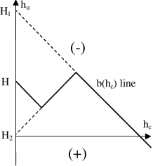
FIG. 1.: Preisach plane with example of state line $b(h_{c})$ generated by the following field history: $-\infty$, $H_{1}$, $H_{2}$, $H$

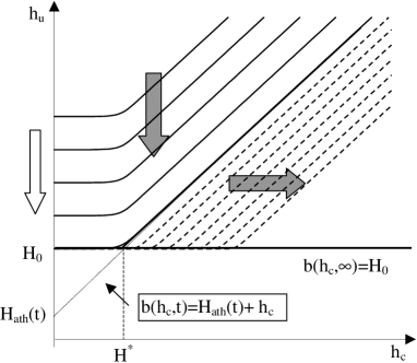
FIG. 2.: State evolution for the field history considered in a magnetic viscosity experiment. The system is prepared by starting from positive saturation ($H\rightarrow\infty$), then bringing the field down to the final value $H_{0}$ at the rate $dH/dt$, and then, from the instant $t=0$, keeping $H_{0}$ constant over time. Continuous lines: sequence of state lines $b(h_{c},t)$ calculated from Eq.(11) in the case where the field $H(t)$ decreases from $+\infty$ at the field rate $dH/dt$. Dashed lines: sequence of state lines $b(h_{c},t)$ calculated from Eq.(10) under constant field $H_{0}$. As time proceeds, $b(h_{c},t)$ approaches the equilibrium state line $b(h_{c},\infty)=H_{0}$ by a front that moves at logarithmic speed. In the region $h_{c}>H^{*}(t)$, the state line can be described as $b(h_{c},t)=H_{ath}(t)+h_{c}$, where the athermal field $H_{ath}(t)$ is given by Eq.(2)

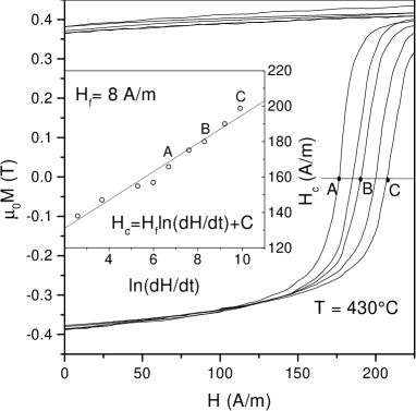
FIG. 3.: Hysteresis loops measured on Fe_73.5Cu₁Nb₃Si_13.5B₉ alloy (Finemet) at T=430^∘C under different field rates from 10 Am^-1s^-1 to 10⁵ Am^-1s^-1. Inset: Corresponding coercive field with best fit obtained from Eq.(1)

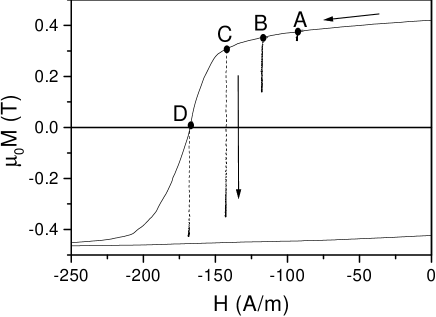
FIG. 4.: Magnetization decay under constant field $H_{0}$ measured on Finemet at T=430^∘C. The different fields $H_{0}$ (-93 Am^-1 (A); -118 Am^-1 (B); -143 Am^-1 (C); -168 Am^-1 (D)) are reached under identical field rate $dH/dt=6.2510^{3}$Am^-1s^-1. The figure shows the extent of decay in 0.5 s (see Fig.6).

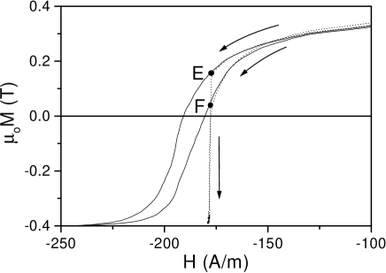
FIG. 5.: Magnetization decay under constant field $H_{0}$ measured on Finemet at T=430^∘C. The same field $H_{0}=-178$Am^-1 is reached at different field rates $dH/dt$ (2 10⁴Am^-1s^-1 (E); 10⁴Am^-1s^-1 (F)). The figure shows the extent of decay in 0.01 s. (see Fig.6)

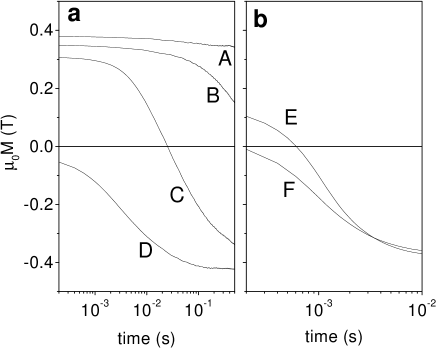
FIG. 6.: Time behavior of the magnetization $M(t)$ for the field histories of Fig.4 (left) and Fig.5 (right).

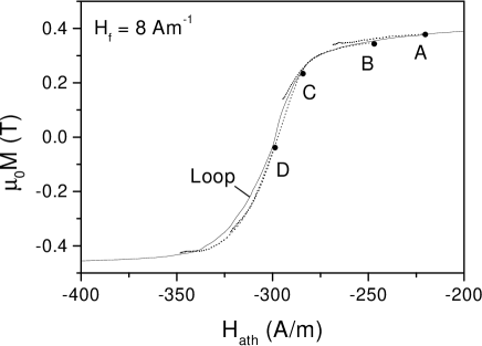
FIG. 7.: Relaxation curves of Fig.6a (broken lines) and hysteresis loop of Fig.4 (solid line) as a function of the field $H_{ath}$ of Eq.(2), calculated assuming $H_{f}=8$Am^-1 and $\tau_{0}=10^{-10}$ s

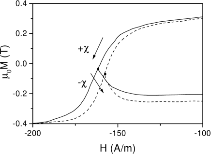
FIG. 8.: Return branches measured on Finemet at T=430^∘C after field reversal at $H=H_{p}$. Continuous lines: $dH/dt$=2 10³ Am^-1s^-1, $H_{p}=-160.5$ Am^-1; broken lines: $dH/dt$=8 10²Am^-1s^-1, $H_{p}=-157.5$ Am^-1.

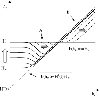
FIG. 9.: State evolution after field reversal at $H=H_{p}$. Continuous lines: when $H$ increases from $H_{p}$ to $H_{0}$ the state line $b(h_{c},t)$ is given by Eq.(6), with Eq.(11) as initial condition. Part B of the state line moves downward even if the field is increasing. Dashed lines: once the field has reached the constant value $H_{0}$ the time dependence of the state line is given by Eq.(10). Relaxation proceeds through the motion of the two fronts indicated by the gray arrows. Part B of the state line can be described as $b(h_{c},t)=H^{+}(t)+h_{c}$, where the $H^{+}(t)$ is given by Eq.(16).

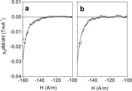
FIG. 10.: Differential susceptibilities measured on Finemet at T=430^∘C after a turning point at $H=H_{p}$. Left: $dH/dt=210^{3}$Am^-1s^-1, $H_{p}=-160.5$ Am^-1. Right: $dH/dt=810^{2}$Am^-1s^-1, $H_{p}=-157.5$ Am^-1. (see Fig.8). Continuous lines: Eq.(3) with $H_{f}=8$Am^-1.

REFERENCES

- [1] K.H.Muller, D.Eckert, A.Hadstein, M.Wolf, S.Collocott and C.Adrikidis, Proc. of the 9th Int. Symposium Magnetic Anisotropy and Coercivity In Rare-Earth Transition Metal Alloys (F.Missell et al. eds.) 381 (1996).
- [2] R. Street and J. Wolley, Proc. Phys. Soc. A62, 562 (1949).
- [3] Y.Estrin, P.G.McCormick, and R.Street, J.Phys.:Cond.Mat. 1, 4845 (1989).
- [4] S.D.Brown, R.Street, R.W.Chantrell, P.W.Haycock and K.O’Grady, J.Appl.Phys. 79, 2594 (1996).
- [5] D.Givord and M. Rossignol, in Rare-earth Iron permanent magnets ( J.M.D.Coey ed.) Oxford University Press 218 (1996).
- [6] Y. Kanay and S. Charap, IEEE Trans. Magn. 27, 4972 (1991).
- [7] R. Chantrell, A. Lyberatos, M. El-Hilo, and K. O’Grady, J.Appl.Phys. 76, 6407 (1994).
- [8] G. Bertotti, Phys. Rev. Lett. 76, 1739 (1996).
- [9] P. Mitcheler, E. Dahlberg, E. Wesseling, and R.M.Roshko, IEEE Trans. Magn. 32, 3185 (1996).
- [10] L.Neel, J. Phys. Rad. 11, 49 (1950).
- [11] F.Preisach, Z.Phys. 94, 277 (1935), (in German).
- [12] J.Souletie, J.Physique 44, 1095 (1983).
- [13] M.LoBue, V.Basso, G.Bertotti, and K.H.Muller, IEEE Trans. Magn. 33, 3862 (1997).
- [14] I. Mayergoyz and C. Korman, J.Appl.Phys. 69, 2128 (1991).
- [15] I.D.Mayergoyz, Mathematical models of hysteresis (Springer, New York, 1991).
- [16] Y.Yoshizawa, S.Oguma, and K.Yamauchi, J.Appl.Phys. 64, 6044 (1988).
- [17] A.Hernando and T. Kulik, Phys.Rev. B 49, 7064 (1994).
- [18] V. Basso, M. LoBue, C. Beatrice, P. Tiberto and G. Bertotti, IEEE Trans. Magn. 34, 1177 (1998).
- [19] E.P.Wohlfarth, J.Phys. F 14, L115 (1994).
- [20] G. Bertotti, Hysteresis in magnetism (Academic press, Boston, 1998).
- [21] A.Hernando, P.Marin, M.Vazquez, J.M.Barandiaran and G.Herzer, Phys.Rev.B 58, 366 (1998).
- [22] P.Bruno, G.Bayereuther, P.Beauvillain, C.Chappert, G.Lugert, D.Renard, J.P.Renard and J.Seiden, J. Appl. Phys. 68, 5759 (1990).