Theory of anomalous magnon softening in ferromagnetic manganites

Abstract

In metallic manganites with low Curie temperatures, a peculiar softening of the magnon spectrum close to the magnetic zone boundary has experimentally been observed. Here we present a theory of the renormalization of the magnetic excitation spectrum in colossal magnetoresistance compounds. The theory is based on the modulation of magnetic exchange bonds by the orbital degree of freedom of double-degenerate $e_{g}$ electrons. The model considered is an orbitally degenerate double-exchange system coupled to Jahn-Teller active phonons which we treat in the limit of strong onsite repulsions. Charge and coupled orbital-lattice fluctuations are identified as the main origin of the unusual softening of the magnetic spectrum.

]

I Introduction

The motion of charge carriers in the metallic phase of manganites establishes a ferromagnetic interaction between spins on neighboring sites. According to the conventional theory of double exchange,[2, 3, 4, 5, 6] the spin dynamics of the ferromagnetic state that evolves at temperatures below the Curie temperature $T_{C}$ is expected to be of nearest-neighbor Heisenberg type. This picture seems to be indeed reasonably accurate for manganese oxides with large values of $T_{C}$, i.e., for compounds whose ferromagnetic metallic phase sustains up to rather high temperatures.[7] However, recent experimental studies indicate marked deviations from this canonical behavior in compounds with low values of $T_{C}$. Quite prominent in this respect are measurements of the spin dynamics of the ferromagnetic manganese oxide Pr_0.63Sr_0.37MnO₃:[8] While exhibiting conventional Heisenberg behavior at small momenta, the dispersion of magnetic excitations (magnons) shows curious softening at the boundary of the Brillouin zone. This observation is of high importance as it indicates that some specific feature of magnetism in manganites has yet to be identified.

A comparison of the magnetic behavior of different manganese oxides further highlights the shortcomings of the double-exchange theory: Assuming the magnon dispersion to be of Heisenberg type, a small-momentum fit to a quadratic dispersion relation $\omega_{\mathchoice{{\hbox{\boldmath$\displaystyle q$}}}{{\hbox{\boldmath$\textstyle q$}}}{{\hbox{\boldmath$\scriptstyle q$}}}{{\hbox{\boldmath$\scriptscriptstyle q$}}}}=Dq^{2}$ yields the spin-wave stiffness $D$; in a conventional Heisenberg system the spin-wave stiffness scales with the strength of magnetic exchange bonds $D\propto J$. Since the latter also controls the Curie temperature $T_{C}\propto J$, the ratio of $D$ and $T_{C}$ is expected to be a universal constant. Manganites, on the other hand, exhibit a pronounced deviation from this behavior: $D/T_{C}$ increases significantly as one goes from compounds with high to compounds with low values of $T_{C}$.[9] The presence of an additional mechanism that controls the magnetic behavior of manganites is to be inferred.

In the present paper, we propose a mechanism to explain the above peculiar magnetic properties of ferromagnetic manganites. Our basic idea is the following: The strength of the ferromagnetic interaction at a given bond strongly depends on the orbital quantum number of $e_{g}$ electrons (see Fig. 1) —

       

FIG. 1.: The $e_{g}$-electron transfer amplitude, which controls the double-exchange interaction $J_{\text{DE}}$, strongly depends on the orbital orientation: Along the $z$ direction, e.g., $d_{3z^{2}-r^{2}}$ electrons (left) can hop into empty sites denoted by a sphere, while the transfer of $d_{x^{2}-y^{2}}$ electrons (right) is forbidden.

along the $z$ direction, e.g., only electrons in $d_{3z^{2}-r^{2}}$ orbitals can hop between sites and hence can participate in double-exchange processes; the transfer of $d_{x^{2}-y^{2}}$ electrons is blocked due to the vanishing overlap with O $2p$ orbitals located in-between two neighboring Mn sites. Temporal fluctuations of $e_{g}$ orbitals may thus modulate the magnetic exchange bonds (see Fig. 2), thereby renormalizing the magnon dispersion. Short-wavelength magnons are most sensitive to these local fluctuations and are affected most strongly.

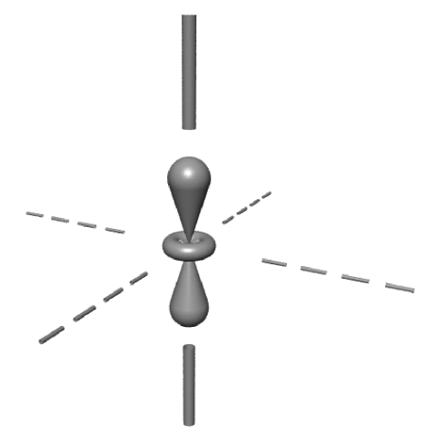
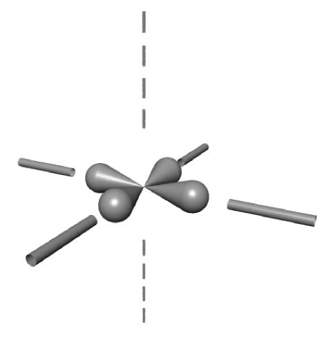
FIG. 2.: Fluctuation of magnetic exchange bonds: Full lines denote active bonds, dashed lines inactive ones.

Quantitatively the modulation of exchange bonds is controlled by the characteristic time scale of orbital fluctuations: If the typical frequency of orbital fluctuations is higher than the one of spins fluctuations, the magnon spectrum remains mostly unrenormalized — the orbital state then effectively enters the spin dynamics only on time average which restores the cubic symmetry of exchange bonds. On the other hand, if orbitals fluctuate slower than spins, the renormalization of the magnon spectrum is most pronounced — the anisotropy imposed upon the magnetic exchange bonds by the orbital degree of freedom now comes into play. The presence of Jahn-Teller phonons enhances this effect by quenching the dynamics of orbitals. The suppression of fluctuations becomes almost complete as orbitals begin to order, resulting in a distinct softening of magnons which we interprete as a precursor effect of static orbital order.

In the following, we calculated the dispersion of one-magnon excitations at zero temperature. We start from an orbitally degenerate Hubbard model that comprises the strongly correlated nature of the Mn $3d$ electrons and the physics of double exchange. The metallic motion of charge carriers establishes magnetic double-exchange bonds which are found to be further contributed to by virtual superexchange processes. Both types of exchange interaction are of ferromagnetic nature in the orbitally degenerate system subject to a strong Hund’s coupling. Employing a $1/S$ expansion of spin and an orbital-liquid scheme [10, 11] to handle correlation effects, three different mechanisms are analyzed with respect to their capability to renormalize the magnon spectrum: scattering of magnons on orbital fluctuations, on charge fluctuations, and on phonons. Within this picture we can successfully reproduce the experimentally observed softening of the magnon dispersion. Furthermore we predict the renormalization effect to become dramatic as static order in the orbital-lattice sector is approached. We note that the renormalization of the magnetic excitation spectrum by optical phonons has recently been investigated by Furukawa.[12]

II Magnetic Exchange Bonds

The main aspects of the physics of manganites, i.e., the correlated motion of itinerant $e_{g}$ electrons and the ferromagnetic interaction of $e_{g}$ spins with a background of localized core spins, is captured by the following orbitally degenerate Hubbard model:

$$H_{\text{Hub}} = -\sum_{\langle ij\rangle_{\gamma}}\sum_{s\alpha\beta}t_{\gamma}^{\alpha\beta}\left(c^{\dagger}_{is\alpha}c_{js\beta}+\text{H.c.}\right)-J_{H}\sum_{i}\mathchoice{{\hbox{\boldmath$\displaystyle S$}}}{{\hbox{\boldmath$\textstyle S$}}}{{\hbox{\boldmath$\scriptstyle S$}}}{{\hbox{\boldmath$\scriptscriptstyle S$}}}^{c}_{i}\mathchoice{{\hbox{\boldmath$\displaystyle s$}}}{{\hbox{\boldmath$\textstyle s$}}}{{\hbox{\boldmath$\scriptstyle s$}}}{{\hbox{\boldmath$\scriptscriptstyle s$}}}_{i}$$ (3)

$$+\sum_{i}\sum_{\alpha}Un_{i\uparrow\alpha}n_{i\downarrow\alpha}$$

$$+\sum_{i}{\sum_{\alpha\neq\beta}}^{\prime}\left(U^{\prime}-J_{H}\hat{P}\right)n_{i\alpha}n_{i\beta},$$

with $\hat{P}=(\mathchoice{{\hbox{\boldmath$\displaystyle s$}}}{{\hbox{\boldmath$\textstyle s$}}}{{\hbox{\boldmath$\scriptstyle s$}}}{{\hbox{\boldmath$\scriptscriptstyle s$}}}_{i\alpha}\mathchoice{{\hbox{\boldmath$\displaystyle s$}}}{{\hbox{\boldmath$\textstyle s$}}}{{\hbox{\boldmath$\scriptstyle s$}}}{{\hbox{\boldmath$\scriptscriptstyle s$}}}_{i\beta}+\frac{3}{4})$. The first term in Eq. (3) describes the intersite transfer of electrons within degenerate $e_{g}$ levels. Here, $c^{\dagger}_{is\alpha}$ creates an $e_{g}$ electrons with spin and orbital quantum numbers $s$ and $\alpha$/$\beta$, respectively. The spatial direction of bonds is specified by $\gamma\in\{x,y,z\}$. One of the important features of the orbitally degenerate model is the nondiagonal structure of the transfer matrices[13]

$\displaystyle t_{x/y}^{\alpha\beta}=t\left(\begin{array}[]{cc}1/4&\mp\sqrt{3}/4\\ \mp\sqrt{3}/4&3/4\end{array}\right),\quad t_{z}^{\alpha\beta}=t\left(\begin{array}[]{cc}1&0\\ 0&0\end{array}\right),$

where we have chosen a representation with respect to the orbital basis $\{|3z^{2}-r^{2}\rangle,|x^{2}-y^{2}\rangle\}$. The second term of Eq. (3) describes the Hund’s coupling between the itinerant $e_{g}$ electrons and the localized core spins $\mathchoice{{\hbox{\boldmath$\displaystyle S$}}}{{\hbox{\boldmath$\textstyle S$}}}{{\hbox{\boldmath$\scriptstyle S$}}}{{\hbox{\boldmath$\scriptscriptstyle S$}}}^{c}_{i}$; the magnitude of this coupling is $J_{H}$. The spin operator $\mathchoice{{\hbox{\boldmath$\displaystyle s$}}}{{\hbox{\boldmath$\textstyle s$}}}{{\hbox{\boldmath$\scriptstyle s$}}}{{\hbox{\boldmath$\scriptscriptstyle s$}}}_{i\alpha}$ acts on $e_{g}$ electrons in orbitals $\alpha$, while $\mathchoice{{\hbox{\boldmath$\displaystyle s$}}}{{\hbox{\boldmath$\textstyle s$}}}{{\hbox{\boldmath$\scriptstyle s$}}}{{\hbox{\boldmath$\scriptscriptstyle s$}}}_{i}=\sum_{\alpha}\mathchoice{{\hbox{\boldmath$\displaystyle s$}}}{{\hbox{\boldmath$\textstyle s$}}}{{\hbox{\boldmath$\scriptstyle s$}}}{{\hbox{\boldmath$\scriptscriptstyle s$}}}_{i\alpha}$ denotes the total $e_{g}$ spin at a given site. Finally, the last two terms in model (3) account for the intra- (inter-) orbital Coulomb interaction $U$ ($U^{\prime}$) and the Hund’s coupling between $e_{g}$ electrons in doubly occupied states. $n_{is\alpha}$ is the number operators of $e_{g}$ electrons in the state defined by $s$ and $\alpha$, and $n_{i\alpha}=\sum_{s}n_{i\alpha}$. Double counting is excluded from the primed sum in the last term of Eq. (3).

In analogy to the transformation from a conventional Hubbard to $t$-$J$ model, Eq. (3) can be projected onto the part of the Hilbert space with no double occupancies in the limit of strong onsite repulsions $U\gg t$ and $(U^{\prime}-J_{H})\gg t$. Doubly occupied states are then allowed only in virtual superexchange processes. Due to the presence of Hund’s coupling, the energy level of these virtual states depends on the spin orientation of core and $e_{g}$ spins — a rich multiplet structure follows.[14] The problem considerably simplifies in the limit of large Hund’s coupling $U,U^{\prime}\gg J_{H}\gg t$ which we believe to be realistic to manganites: Transitions to the lowest-lying intermediate state with energy $U_{1}=U^{\prime}-J_{H}$ in which core and $e_{g}$ spins are in a high-spin configuration then dominate; doubly occupied sites with different spin structures lie higher by an energy of the order of $\propto J_{H}$ and can be neglected. We hence obtain the following $t$-$J$ Hamiltonian:

$$H_{tJ} = -\sum_{\langle ij\rangle_{\gamma}}\sum_{s\alpha\beta}t_{\gamma}^{\alpha\beta}\left(\hat{c}^{\dagger}_{is\alpha}\hat{c}_{js\beta}+\text{H.c.}\right)-J_{H}\sum_{i}\mathchoice{{\hbox{\boldmath$\displaystyle S$}}}{{\hbox{\boldmath$\textstyle S$}}}{{\hbox{\boldmath$\scriptstyle S$}}}{{\hbox{\boldmath$\scriptscriptstyle S$}}}_{i}^{c}\mathchoice{{\hbox{\boldmath$\displaystyle s$}}}{{\hbox{\boldmath$\textstyle s$}}}{{\hbox{\boldmath$\scriptstyle s$}}}{{\hbox{\boldmath$\scriptscriptstyle s$}}}_{i}$$ (5)

$$-J_{\text{SE}}\sum_{\langle ij\rangle_{\gamma}}\left(\frac{1}{4}-\tau_{i}^{\gamma}\tau_{j}^{\gamma}\right)\left[\mathchoice{{\hbox{\boldmath$\displaystyle S$}}}{{\hbox{\boldmath$\textstyle S$}}}{{\hbox{\boldmath$\scriptstyle S$}}}{{\hbox{\boldmath$\scriptscriptstyle S$}}}_{i}\mathchoice{{\hbox{\boldmath$\displaystyle S$}}}{{\hbox{\boldmath$\textstyle S$}}}{{\hbox{\boldmath$\scriptstyle S$}}}{{\hbox{\boldmath$\scriptscriptstyle S$}}}_{j}+S(S+1)\right]n_{i}n_{j}.$$

The first two terms in Eq. (LABEL:HTJ) describe the double-exchange mechanism in the limit of strong onsite repulsions. All double occupancies of $e_{g}$ electrons are projected out by the constrained operators $\hat{c}^{\dagger}_{is\alpha}=c^{\dagger}_{is\alpha}(1-n_{i})$ which act only on empty sites. The third term in Eq. (LABEL:HTJ) describes the superexchange interaction between singly occupied sites. The strength of this interaction is controlled by $J_{\text{SE}}=(2t^{2}/U_{1})[S(2S+1)]^{-1}$, where $S$ denotes the total onsite spin of $3d$ electrons. It is important to note that in the present model with large $J_{H}$, superexchange is of ferromagnetic nature. This stems from the fact that Hund’s coupling forbids any double occupancy of a single $e_{g}$ orbital. Pauli’s exclusion principle, which is responsible for the antiferromagnetic nature of conventional superexchange, is therefore ineffective in dictating the spin structure of the virtual state. Rather, the spin orientation in the intermediate state is controlled by Hund’s coupling which favors a ferromagnetic alignment of spins. The superexchange term in Eq. (LABEL:HTJ) exhibits yet another peculiar feature: The amplitude of superexchange processes depends on the orbital states of the $e_{g}$ electrons involved. This information enters via the orbital pseudospin operators

$\displaystyle\tau_{i}^{x/y}=-\frac{1}{4}\left(\sigma_{i}^{z}\pm\sqrt{3}\sigma_{i}^{x}\right),\quad\tau_{i}^{z}=\frac{1}{2}\sigma_{i}^{z},$

where the Pauli matrices $\sigma_{i}^{x/z}$ act on the orbital subspace; the factor $(\frac{1}{4}-\tau_{i}^{\gamma}\tau_{j}^{\gamma})$ in Eq. (LABEL:HTJ) accounts for the specific nondiagonal structure of the transfer matrices $t_{\gamma}^{\alpha\beta}$ and ensures that no double occupancy of a single orbital occurs which would be forbidden by Pauli’s exclusion principle and the large Hund’s coupling. We finally note that superexchange processes in an orbitally degenerate system have also been studied by Feiner and Oleś.[14] In the limit of large $J_{H}$ the expression obtained by these authors maps onto the superexchange term of Eq. (LABEL:HTJ) for the special case $S=2$.

In the following, double-exchange and superexchange interactions which are jointly responsible for ferromagnetism in manganites are discussed in more detail.

A Double-Exchange Bonds

We begin by analyzing the kinetic term of Hamiltonian (LABEL:HTJ),

$$H_{t}=-\sum_{\langle ij\rangle_{\gamma}}\sum_{s\alpha\beta}t_{\gamma}^{\alpha\beta}\left(\hat{c}^{\dagger}_{is\alpha}\hat{c}_{js\beta}+\text{H.c.}\right)-J_{H}\sum_{i}\mathchoice{{\hbox{\boldmath$\displaystyle S$}}}{{\hbox{\boldmath$\textstyle S$}}}{{\hbox{\boldmath$\scriptstyle S$}}}{{\hbox{\boldmath$\scriptscriptstyle S$}}}_{i}^{c}\mathchoice{{\hbox{\boldmath$\displaystyle s$}}}{{\hbox{\boldmath$\textstyle s$}}}{{\hbox{\boldmath$\scriptstyle s$}}}{{\hbox{\boldmath$\scriptscriptstyle s$}}}_{i},$$ (7)

which establishes the double-exchange mechanism in the correlated system. Due to the strong Hund’s coupling, core spins $\mathchoice{{\hbox{\boldmath$\displaystyle S$}}}{{\hbox{\boldmath$\textstyle S$}}}{{\hbox{\boldmath$\scriptstyle S$}}}{{\hbox{\boldmath$\scriptscriptstyle S$}}}^{c}$ and itinerant $e_{g}$ spins $\textstyle s$ are not independent of each other; rather a high-spin state with total onsite spin $S=S^{c}+\frac{1}{2}$ is formed. This unification of band and local spin subspaces suggests to decompose the $e_{g}$ electron into its spin and orbital/charge components. The $e_{g}$ spin can then be absorbed into the total spin, allowing an independent treatment of spin and orbital/charge degrees of freedom (see Fig. 3).

FIG. 3.: The itinerant $e_{g}$ spin (top left) interacts with the localized core spins (bottom left) via Hund’s coupling. In the limit $J_{H}\gg t$, the former can be separated from the orbital and charge degrees of freedom of the $e_{g}$ electron (circle) and can be absorbed into the total spin (bottom right).

The procedure of this separation scheme is the following: In a first step we introduce Schwinger bosons $d_{i\uparrow}$ and $d_{i\downarrow}$ (see, e.g., Ref. [15]) to describe the $e_{g}$ spin

$$s_{i}^{+}=d^{\dagger}_{i\uparrow}d_{i\downarrow},\quad s_{i}^{-}=d^{\dagger}_{i\downarrow}d_{i\uparrow},$$

$$s_{i}^{z}=\frac{1}{2}(d^{\dagger}_{i\uparrow}d_{i\uparrow}-d^{\dagger}_{i\downarrow}d_{i\downarrow}),$$

as well as Schwinger bosons $D^{\dagger}_{i\uparrow}$ and $D^{\dagger}_{i\downarrow}$ to model the total onsite spin

$$S_{i}^{+}=D^{\dagger}_{i\uparrow}D_{i\downarrow},\quad S_{i}^{-}=D^{\dagger}_{i\downarrow}D_{i\uparrow},$$

$$S_{i}^{z}=\frac{1}{2}(D^{\dagger}_{i\uparrow}D_{i\uparrow}-D^{\dagger}_{i\downarrow}D_{i\downarrow}).$$

These auxiliary particles are subject to the following constraints that depend on the $e_{g}$ occupation number $n_{i}$:

$$d^{\dagger}_{i\uparrow}d_{i\uparrow}+d^{\dagger}_{i\downarrow}d_{i\downarrow} = n_{i},$$ (8)

$$D^{\dagger}_{i\uparrow}D_{i\uparrow}+D^{\dagger}_{i\downarrow}D_{i\downarrow} = 2S-1+n_{i}.$$ (9)

The creation and destruction operators for $e_{g}$ electrons can then be expressed in terms of spinless fermions $c_{i\alpha}$ which carry charge and orbital pseudospin and Schwinger bosons which carry spin:

$\displaystyle c_{is\alpha}=c_{i\alpha}d_{is}.$

The kinetic-energy Hamiltonian (7) now describes the transfer of pairs of spinless fermions and Schwinger bosons:

$$H_{t}=-\sum_{\langle ij\rangle_{\gamma}}\sum_{s\alpha\beta}t_{\gamma}^{\alpha\beta}\left(\hat{c}^{\dagger}_{i\alpha}\hat{c}_{j\beta}d^{\dagger}_{is}d_{js}+\text{H.c.}\right)-J_{H}\sum_{i}\mathchoice{{\hbox{\boldmath$\displaystyle S$}}}{{\hbox{\boldmath$\textstyle S$}}}{{\hbox{\boldmath$\scriptstyle S$}}}{{\hbox{\boldmath$\scriptscriptstyle S$}}}_{i}^{c}\mathchoice{{\hbox{\boldmath$\displaystyle s$}}}{{\hbox{\boldmath$\textstyle s$}}}{{\hbox{\boldmath$\scriptstyle s$}}}{{\hbox{\boldmath$\scriptscriptstyle s$}}}_{i}.$$ (10)

The Bose operators are subject to the constraint (8) that enforces the operators $d_{is}$ and $d^{\dagger}_{is}$ to act only on projected Hilbert spaces with one or zero Schwinger bosons, respectively. Our aim is to absorb the $e_{g}$ spin into the total spin, which requires to map the $e_{g}$ operators $d_{is}$ onto operators $D_{is}$ for the total spin. This is done by comparing the matrix elements of the two types of operators. On the one hand, keeping in mind that Hund’s rule enforces the onsite spins to be always in a total-spin-symmetric state, the only nonvanishing matrix elements of the $d_{is}$ operators are

$$\Big{\langle}S-\frac{1}{2},m-\frac{1}{2}\Big{|}d_{\uparrow}\Big{|}S,m\Big{\rangle} = \sqrt{(S+m)/(2S)},$$ (11)

$$\Big{\langle}S-\frac{1}{2},m+\frac{1}{2}\Big{|}d_{\downarrow}\Big{|}S,m\Big{\rangle} = \sqrt{(S-m)/(2S)}.$$ (12)

In deriving the above expressions we have used the Clebsch-Gordan coefficients $\langle S^{c},m^{c};m^{e}|S,m\rangle$ to decompose the total-spin state $|S,m\rangle$ into core- and $e_{g}$-spin states $|S^{c},m^{c};m^{e}\rangle$ with $m^{e}=\uparrow/\downarrow$. These coefficients are given by

$$\langle S-\frac{1}{2},m-\mbox{$\frac{1}{2}$};\uparrow|S,m\rangle = \left[\frac{S+m}{2S}\right]^{1/2},$$

$$\langle S-\frac{1}{2},m+\frac{1}{2};\downarrow|S,m\rangle = \left[\frac{S-m}{2S}\right]^{1/2}.$$

On the other hand, the matrix elements of the $D_{is}$ operators are

$$\Big{\langle}S-\frac{1}{2},m-\frac{1}{2}\Big{|}D_{\uparrow}\Big{|}S,m\Big{\rangle} = \sqrt{(S+m)},$$ (13)

$$\Big{\langle}S-\frac{1}{2},m+\frac{1}{2}\Big{|}D_{\downarrow}\Big{|}S,m\Big{\rangle} = \sqrt{(S-m)}.$$ (14)

All other matrix elements vanish due to the constraint of Eq. (9). By comparing Eqs. (11)-(12) with Eqs. (13)-(14) we obtain the mapping

$\displaystyle d_{is}=\frac{1}{\sqrt{2S}}D_{is}.$

Hamiltonian (10) can hence be rewritten in terms of total-spin operators $D_{is}$:

$$H_{t}=-\frac{1}{2S}\sum_{\langle ij\rangle_{\gamma}}\sum_{s\alpha\beta}t_{\gamma}^{\alpha\beta}\left(\hat{c}^{\dagger}_{i\alpha}\hat{c}_{j\beta}D^{\dagger}_{is}D_{js}+\text{H.c.}\right).$$ (15)

The Hund’s coupling term of Eq. (10) has been dropped here as its presence is implied by the spin construction employed above. This completes the separation of spin from the charge/orbital quantum numbers of $e_{g}$ electrons.

At low temperatures the magnetic moment of ferromagnetic manganites studied here is almost fully saturated. It is therefore reasonable to expand Eq. (15) around a ferromagnetic groundstate. Technically this is done by condensing the spin-up Schwinger bosons (assuming the ferromagnetic moment to point along this direction) and by treating spin-wave excitations around this groundstate in leading order of $1/S$. Introducing magnon operators $b_{i}$, the following relations hold:

$$D_{i\uparrow} = \sqrt{2S-b^{\dagger}_{i}b_{i}}\approx\sqrt{2S}\left(1-\frac{1}{4S}b^{\dagger}_{i}b_{i}\right),$$

$$D_{i\downarrow} = b_{i}.$$

This spin representation fixes the number of Schwinger bosons per site to $2S$. The essence of the $1/S$ expansion is to consider the presence of a hole as a small perturbation which changes the spin projection $S^{z}$ but not the spin magnitude $S$. Employing magnon operators, the kinetic-energy Hamiltonian (15) hence becomes

$$H_{t} = -\sum_{\langle ij\rangle_{\gamma}}\sum_{\alpha\beta}t_{\gamma}^{\alpha\beta}\hat{c}^{\dagger}_{i\alpha}\hat{c}_{j\beta}$$ (18)

$$+\frac{1}{2S}\sum_{\langle ij\rangle_{\gamma}}\sum_{\alpha\beta}t_{\gamma}^{\alpha\beta}\hat{c}^{\dagger}_{i\alpha}\hat{c}_{j\beta}\Big{(}\frac{1}{2}b^{\dagger}_{i}b_{i}+\frac{1}{2}b^{\dagger}_{j}b_{j}-b^{\dagger}_{i}b_{j}\Big{)}$$

$$+\text{H.c.}$$

The first term of Eq. (18) describes the motion of strongly correlated fermions in a ferromagnetic background. The second term controls the dynamics of spin excitations in the magnetic background and the interaction of these excitations with the fermionic sector.

At small magnon numbers, i.e., at low temperatures $T\ll T_{C}$, Eq. (18) can be mapped onto the following expression for the magnetic double-exchange bonds:

$$H_{t} = -\sum_{\langle ij\rangle_{\gamma}}\sum_{\alpha\beta}t_{\gamma}^{\alpha\beta}\hat{c}^{\dagger}_{i\alpha}\hat{c}_{j\beta}\Big{[}\frac{3}{4}+\frac{1}{4S^{2}}\left(S_{i}^{z}S_{j}^{z}+S_{i}^{-}S_{j}^{+}\right)\Big{]}$$ (20)

$$+\text{H.c.}$$

Equation (20) highlights an important point: The strength of double-exchange bonds is a fluctuating complex quantity. Only when treating the orbital and charge sectors on average, i.e., when replacing the bond operators $\hat{c}^{\dagger}_{i\alpha}\hat{c}_{i\beta}$ by their mean-field value $\langle\hat{c}^{\dagger}_{i\alpha}\hat{c}_{i\beta}\rangle$, an effective Heisenberg model as in a conventional mean-treatment of double exchange is obtained: $H=J_{\text{DE}}\sum_{\langle ij\rangle}\mathchoice{{\hbox{\boldmath$\displaystyle S$}}}{{\hbox{\boldmath$\textstyle S$}}}{{\hbox{\boldmath$\scriptstyle S$}}}{{\hbox{\boldmath$\scriptscriptstyle S$}}}_{i}\mathchoice{{\hbox{\boldmath$\displaystyle S$}}}{{\hbox{\boldmath$\textstyle S$}}}{{\hbox{\boldmath$\scriptstyle S$}}}{{\hbox{\boldmath$\scriptscriptstyle S$}}}_{j}$ with $J_{\text{DE}}=(2S^{2})^{-1}\sum_{\alpha\beta}t_{\gamma}^{\alpha\beta}\langle\hat{c}^{\dagger}_{i\alpha}\hat{c}_{j\beta}\rangle$. In Section III we investigate in more detail the modification of the mean-field picture by fluctuations in the bond amplitude.

It is interesting to turn to the limit of classical spins shortly. Replacing the spin operators in Eq. (20) by their classical counterparts $S^{z}=S\cos\theta$ and $S^{\pm}=S\sin\theta e^{\mp i\phi}$, an effective fermionic model is obtained:

$$H_{t}=-\sum_{\langle ij\rangle_{\gamma}}\sum_{\alpha\beta}\tilde{t}_{\gamma}^{\alpha\beta}\hat{c}^{\dagger}_{i\alpha}\hat{c}_{j\beta}+\text{H.c.}$$ (21)

This model exhibits an unconventional phase-dependent hopping amplitude:[16]

$\displaystyle\tilde{t}_{\gamma}^{\alpha\beta}=t_{\gamma}^{\alpha\beta}\Big{[}\frac{3}{4}+\frac{1}{4}\left(\sin\theta_{i}\sin\theta_{j}+\sin\theta_{i}\sin\theta_{j}e^{i(\phi_{i}-\phi_{j})}\right)\Big{]}.$

A similar result has been discussed in Refs. [17, 18] in terms of a Berry-phase effect.

B Superexchange Bonds

At low- and intermediate-doping levels, virtual charge-transfer processes across the Hubbard gap becomes of importance. These superexchange processes establish an intersite interaction, which in the limit of a strong Hund’s coupling is described by [see Eq. (LABEL:HTJ)]:

$$H_{J}=-J_{\text{SE}}\sum_{\langle ij\rangle_{\gamma}}\left(\frac{1}{4}-\tau_{i}^{\gamma}\tau_{j}^{\gamma}\right)\left[\mathchoice{{\hbox{\boldmath$\displaystyle S$}}}{{\hbox{\boldmath$\textstyle S$}}}{{\hbox{\boldmath$\scriptstyle S$}}}{{\hbox{\boldmath$\scriptscriptstyle S$}}}_{i}\mathchoice{{\hbox{\boldmath$\displaystyle S$}}}{{\hbox{\boldmath$\textstyle S$}}}{{\hbox{\boldmath$\scriptstyle S$}}}{{\hbox{\boldmath$\scriptscriptstyle S$}}}_{j}+S(S+1)\right]n_{i}n_{j}.$$ (22)

As mentioned above, superexchange is of ferromagnetic nature in the orbitally degenerate system with strong onsite correlations. Double exchange and superexchange therefore act together in establishing the ferromagnetic exchange links in metallic manganites.[19]

Following the discussion on double-exchange bonds we express the spin operators in Eq. (22) in terms of magnon operators $b_{i}$. This leads to

$$H_{J} = SJ_{\text{SE}}\sum_{\langle ij\rangle_{\gamma}}\left(\frac{1}{4}-\tau_{i}^{\gamma}\tau_{j}^{\gamma}\right)n_{i}n_{j}$$ (24)

$$\times\Big{[}\Big{(}\frac{1}{2}b^{\dagger}_{i}b_{i}+\frac{1}{2}b^{\dagger}_{j}b_{j}-b^{\dagger}_{i}b_{j}+\text{H.c.}\Big{)}-(2S+1)\Big{]}.$$

Equation (LABEL:HJB) describes the interaction between orbital fluctuations and the magnetic sector of the Hilbert space.[20] The phase dependence exhibited by the double-exchange counterpart Eq. (18) is absent here. This is due to the fact that superexchange is a second-order process which depends only the amplitude but not on the phase of the transfer amplitude.

III Magnon Dispersion

In the previous section, the role of double-exchange and superexchange processes in promoting ferromagnetic exchange bonds in manganites was discussed. At intermediate-doping levels these exchange interactions induce a ferromagnetic groundstate in a variety of manganese oxides. We now turn to analyze the propagation of magnetic excitations in this ferromagnetic phase, namely by deducing the dispersion relation of single-magnon excitations.

In a first step, we derive the correct operator for creating a magnetic excitation in hole-doped double-exchange systems. It has to account for the fact that the total onsite spin depends on whether a hole or an $e_{g}$ electron is present at that site: The spin number is $S-\frac{1}{2}$ in the former and $S$ in the latter case. This difference in the spin number was neglected in the $1/S$ expansion employed in Sec. II. Here this approximation is no longer valid, which requires a rescaling of the magnon operators $b_{i}$. In general, a spin excitation is created by the operator $S_{i}^{+}$. Expressing this operator in terms of Schwinger bosons $S^{+}_{i}=D^{\dagger}_{i\uparrow}D_{i\downarrow}$, condensing $D_{i\uparrow}$, and mapping $D_{i\downarrow}$ onto the magnon operator $b_{i}$, the following representation is obtained:

$\displaystyle S^{+}_{i}=\left\{\begin{array}[]{ll}\displaystyle\sqrt{2S}\;b_{i},&\text{for sites with $e_{g}$ electron},\\ \displaystyle\sqrt{2S-1}\;b_{i},&\text{for sites with hole}.\end{array}\right.$

Assuming $S$ to be the “natural” spin number of the system, the magnon operator $b_{i}$ hence has to be rescaled by a factor $[(2S-1)/(2S)]^{1/2}$ when being applied to hole sites:

$\displaystyle B_{i}=\left\{\begin{array}[]{ll}\displaystyle b_{i},&\text{for sites with $e_{g}$ electron},\\ \displaystyle\sqrt{(2S-1)/(2S)}\;b_{i},&\text{for sites with hole}.\end{array}\right.$

The general magnon operator that automatically probes the presence of an $e_{g}$ electron can finally be written as

$$B_{i} = b_{i}\Bigg{[}n_{i}+\sqrt{\frac{2S-1}{2S}}(1-n_{i})\Bigg{]}$$

$$\approx b_{i}-\frac{1}{4S}(1-n_{i})\;b_{i},$$

where $n_{i}$ is the number operator of $e_{g}$ electrons. $B_{i}$ represents the true Goldstone operator of hole-doped double-exchange systems. Its composite character comprises local and itinerant spin features which is a consequence of the fact that static core and mobile $e_{g}$ electrons together form the total onsite spin. While the itinerant part of $B_{i}$ is of order $1/S$ only, it nevertheless is of crucial importance to ensure consistency of the spin dynamics with the Goldstone theorem, i.e., to yield an excitation mode whose energy vanishes at zero-momentum.

Having derived the correct magnon operator for doped double-exchange systems, we now study the propagation of the magnetic excitations it creates. The link between sites that allows a local excitation to spread throughout the system is established by the exchange-bond Hamiltonians (18) and (LABEL:HJB). At low temperatures the dynamics of spin waves which hence develop is captured by the single-magnon dispersion. The important question we are interested in is the following: To which extent is the magnon spectrum affected by fluctuations in the exchange bonds? To answer this question we express the full magnon spectrum $\tilde{\omega}_{\mathchoice{{\hbox{\boldmath$\displaystyle p$}}}{{\hbox{\boldmath$\textstyle p$}}}{{\hbox{\boldmath$\scriptstyle p$}}}{{\hbox{\boldmath$\scriptscriptstyle p$}}}}$ in terms of the conventional mean-field dispersion $\omega_{\mathchoice{{\hbox{\boldmath$\displaystyle p$}}}{{\hbox{\boldmath$\textstyle p$}}}{{\hbox{\boldmath$\scriptstyle p$}}}{{\hbox{\boldmath$\scriptscriptstyle p$}}}}$ and the magnon selfenergy $\Sigma(\omega,\mathchoice{{\hbox{\boldmath$\displaystyle p$}}}{{\hbox{\boldmath$\textstyle p$}}}{{\hbox{\boldmath$\scriptstyle p$}}}{{\hbox{\boldmath$\scriptscriptstyle p$}}})$:

$$\tilde{\omega}_{\mathchoice{{\hbox{\boldmath$\displaystyle p$}}}{{\hbox{\boldmath$\textstyle p$}}}{{\hbox{\boldmath$\scriptstyle p$}}}{{\hbox{\boldmath$\scriptscriptstyle p$}}}}=\omega_{\mathchoice{{\hbox{\boldmath$\displaystyle p$}}}{{\hbox{\boldmath$\textstyle p$}}}{{\hbox{\boldmath$\scriptstyle p$}}}{{\hbox{\boldmath$\scriptscriptstyle p$}}}}+\text{Re}[\Sigma(\omega_{\mathchoice{{\hbox{\boldmath$\displaystyle p$}}}{{\hbox{\boldmath$\textstyle p$}}}{{\hbox{\boldmath$\scriptstyle p$}}}{{\hbox{\boldmath$\scriptscriptstyle p$}}}},\mathchoice{{\hbox{\boldmath$\displaystyle p$}}}{{\hbox{\boldmath$\textstyle p$}}}{{\hbox{\boldmath$\scriptstyle p$}}}{{\hbox{\boldmath$\scriptscriptstyle p$}}})].$$ (26)

Fluctuation are considered only on average in the former but are explicitly accounted for in the latter term. The mean-field dispersion $\omega_{\mathchoice{{\hbox{\boldmath$\displaystyle p$}}}{{\hbox{\boldmath$\textstyle p$}}}{{\hbox{\boldmath$\scriptstyle p$}}}{{\hbox{\boldmath$\scriptscriptstyle p$}}}}$ as well as the scattering vertices needed to construct $\Sigma(\omega,\mathchoice{{\hbox{\boldmath$\displaystyle p$}}}{{\hbox{\boldmath$\textstyle p$}}}{{\hbox{\boldmath$\scriptstyle p$}}}{{\hbox{\boldmath$\scriptscriptstyle p$}}})$ can be derived by commuting the magnon operator $B_{i}$ with the Hamiltonian. To be specific we explicitly perform this commutation, for now restricting ourselves to the double-exchange Hamiltonian $H_{t}$ given by Eq. (18). In the momentum representation we obtain

$$[B_{\mathchoice{{\hbox{\boldmath$\displaystyle p$}}}{{\hbox{\boldmath$\textstyle p$}}}{{\hbox{\boldmath$\scriptstyle p$}}}{{\hbox{\boldmath$\scriptscriptstyle p$}}}},H_{t}] = \omega_{\mathchoice{{\hbox{\boldmath$\displaystyle p$}}}{{\hbox{\boldmath$\textstyle p$}}}{{\hbox{\boldmath$\scriptstyle p$}}}{{\hbox{\boldmath$\scriptscriptstyle p$}}}}B_{\mathchoice{{\hbox{\boldmath$\displaystyle p$}}}{{\hbox{\boldmath$\textstyle p$}}}{{\hbox{\boldmath$\scriptstyle p$}}}{{\hbox{\boldmath$\scriptscriptstyle p$}}}}$$ (28)

$$+\frac{t}{2S}\sum_{\mathchoice{{\hbox{\boldmath$\displaystyle q$}}}{{\hbox{\boldmath$\textstyle q$}}}{{\hbox{\boldmath$\scriptstyle q$}}}{{\hbox{\boldmath$\scriptscriptstyle q$}}}}\sum_{\alpha\beta}A^{\alpha\beta}_{\mathchoice{{\hbox{\boldmath$\displaystyle p$}}}{{\hbox{\boldmath$\textstyle p$}}}{{\hbox{\boldmath$\scriptstyle p$}}}{{\hbox{\boldmath$\scriptscriptstyle p$}}}}(\mathchoice{{\hbox{\boldmath$\displaystyle k$}}}{{\hbox{\boldmath$\textstyle k$}}}{{\hbox{\boldmath$\scriptstyle k$}}}{{\hbox{\boldmath$\scriptscriptstyle k$}}})\hat{c}^{\dagger}_{\mathchoice{{\hbox{\boldmath$\displaystyle k$}}}{{\hbox{\boldmath$\textstyle k$}}}{{\hbox{\boldmath$\scriptstyle k$}}}{{\hbox{\boldmath$\scriptscriptstyle k$}}}\alpha}\hat{c}_{\mathchoice{{\hbox{\boldmath$\displaystyle k$}}}{{\hbox{\boldmath$\textstyle k$}}}{{\hbox{\boldmath$\scriptstyle k$}}}{{\hbox{\boldmath$\scriptscriptstyle k$}}}-\mathchoice{{\hbox{\boldmath$\displaystyle q$}}}{{\hbox{\boldmath$\textstyle q$}}}{{\hbox{\boldmath$\scriptstyle q$}}}{{\hbox{\boldmath$\scriptscriptstyle q$}}},\beta}B_{\mathchoice{{\hbox{\boldmath$\displaystyle p$}}}{{\hbox{\boldmath$\textstyle p$}}}{{\hbox{\boldmath$\scriptstyle p$}}}{{\hbox{\boldmath$\scriptscriptstyle p$}}}+\mathchoice{{\hbox{\boldmath$\displaystyle q$}}}{{\hbox{\boldmath$\textstyle q$}}}{{\hbox{\boldmath$\scriptstyle q$}}}{{\hbox{\boldmath$\scriptscriptstyle q$}}}}.$$

The two terms on the r.h.s. of Eq. (28) correspond to an expansion of the bond operators $\hat{c}^{\dagger}_{i\alpha}\hat{c}_{j\beta}$ around their average value:

$\displaystyle\hat{c}^{\dagger}_{i\alpha}\hat{c}_{j\beta}\rightarrow\langle\hat{c}^{\dagger}_{i\alpha}\hat{c}_{j\beta}\rangle+\delta\left(\hat{c}^{\dagger}_{i\alpha}\hat{c}_{j\beta}\right).$

The mean-field magnon dispersion $\omega_{\mathchoice{{\hbox{\boldmath$\displaystyle p$}}}{{\hbox{\boldmath$\textstyle p$}}}{{\hbox{\boldmath$\scriptstyle p$}}}{{\hbox{\boldmath$\scriptscriptstyle p$}}}}$ in the first term of Eq. (28) is of conventional nearest-neighbor Heisenberg form

$$\omega_{\mathchoice{{\hbox{\boldmath$\displaystyle p$}}}{{\hbox{\boldmath$\textstyle p$}}}{{\hbox{\boldmath$\scriptstyle p$}}}{{\hbox{\boldmath$\scriptscriptstyle p$}}}}=zD(1-\gamma_{\mathchoice{{\hbox{\boldmath$\displaystyle p$}}}{{\hbox{\boldmath$\textstyle p$}}}{{\hbox{\boldmath$\scriptstyle p$}}}{{\hbox{\boldmath$\scriptscriptstyle p$}}}}),$$ (29)

with the form factor $\gamma_{\mathchoice{{\hbox{\boldmath$\displaystyle p$}}}{{\hbox{\boldmath$\textstyle p$}}}{{\hbox{\boldmath$\scriptstyle p$}}}{{\hbox{\boldmath$\scriptscriptstyle p$}}}}=z^{-1}\sum_{\mathchoice{{\hbox{\boldmath$\displaystyle\delta$}}}{{\hbox{\boldmath$\textstyle\delta$}}}{{\hbox{\boldmath$\scriptstyle\delta$}}}{{\hbox{\boldmath$\scriptscriptstyle\delta$}}}}\exp(i\mathchoice{{\hbox{\boldmath$\displaystyle p$}}}{{\hbox{\boldmath$\textstyle p$}}}{{\hbox{\boldmath$\scriptstyle p$}}}{{\hbox{\boldmath$\scriptscriptstyle p$}}}\mathchoice{{\hbox{\boldmath$\displaystyle\delta$}}}{{\hbox{\boldmath$\textstyle\delta$}}}{{\hbox{\boldmath$\scriptstyle\delta$}}}{{\hbox{\boldmath$\scriptscriptstyle\delta$}}})$, $z=6$, and the spin-wave stiffness constant is $D=SJ_{\text{DE}}$. On this mean-field level the strength of the exchange bonds depends on the orbital and charge degrees of freedom only on average: $J_{\text{DE}}=(2S^{2})^{-1}\sum_{\alpha\beta}t_{\gamma}^{\alpha\beta}\langle\hat{c}^{\dagger}_{i\alpha}\hat{c}_{j\beta}\rangle$. The second term in Eq. (28) is the scattering vertex needed to construct the magnon selfenergy $\Sigma(\omega,\mathchoice{{\hbox{\boldmath$\displaystyle p$}}}{{\hbox{\boldmath$\textstyle p$}}}{{\hbox{\boldmath$\scriptstyle p$}}}{{\hbox{\boldmath$\scriptscriptstyle p$}}})$. It describes the interaction between magnons and orbital/charge fluctuations. The vertex function is

$\displaystyle A^{\alpha\beta}_{\mathchoice{{\hbox{\boldmath$\displaystyle p$}}}{{\hbox{\boldmath$\textstyle p$}}}{{\hbox{\boldmath$\scriptstyle p$}}}{{\hbox{\boldmath$\scriptscriptstyle p$}}}}(\mathchoice{{\hbox{\boldmath$\displaystyle k$}}}{{\hbox{\boldmath$\textstyle k$}}}{{\hbox{\boldmath$\scriptstyle k$}}}{{\hbox{\boldmath$\scriptscriptstyle k$}}})=\gamma^{\alpha\beta}_{\mathchoice{{\hbox{\boldmath$\displaystyle k$}}}{{\hbox{\boldmath$\textstyle k$}}}{{\hbox{\boldmath$\scriptstyle k$}}}{{\hbox{\boldmath$\scriptscriptstyle k$}}}}-\gamma^{\alpha\beta}_{\mathchoice{{\hbox{\boldmath$\displaystyle k$}}}{{\hbox{\boldmath$\textstyle k$}}}{{\hbox{\boldmath$\scriptstyle k$}}}{{\hbox{\boldmath$\scriptscriptstyle k$}}}+\mathchoice{{\hbox{\boldmath$\displaystyle p$}}}{{\hbox{\boldmath$\textstyle p$}}}{{\hbox{\boldmath$\scriptstyle p$}}}{{\hbox{\boldmath$\scriptscriptstyle p$}}}},$

with the form factor $\gamma_{\mathchoice{{\hbox{\boldmath$\displaystyle k$}}}{{\hbox{\boldmath$\textstyle k$}}}{{\hbox{\boldmath$\scriptstyle k$}}}{{\hbox{\boldmath$\scriptscriptstyle k$}}}}^{\alpha\beta}=(zt)^{-1}\sum_{\mathchoice{{\hbox{\boldmath$\displaystyle\delta$}}}{{\hbox{\boldmath$\textstyle\delta$}}}{{\hbox{\boldmath$\scriptstyle\delta$}}}{{\hbox{\boldmath$\scriptscriptstyle\delta$}}}}t_{\delta}^{\alpha\beta}\exp(i\mathchoice{{\hbox{\boldmath$\displaystyle k$}}}{{\hbox{\boldmath$\textstyle k$}}}{{\hbox{\boldmath$\scriptstyle k$}}}{{\hbox{\boldmath$\scriptscriptstyle k$}}}\mathchoice{{\hbox{\boldmath$\displaystyle\delta$}}}{{\hbox{\boldmath$\textstyle\delta$}}}{{\hbox{\boldmath$\scriptstyle\delta$}}}{{\hbox{\boldmath$\scriptscriptstyle\delta$}}})$. The vertex function $A^{\alpha\beta}_{\mathchoice{{\hbox{\boldmath$\displaystyle p$}}}{{\hbox{\boldmath$\textstyle p$}}}{{\hbox{\boldmath$\scriptstyle p$}}}{{\hbox{\boldmath$\scriptscriptstyle p$}}}}(\mathchoice{{\hbox{\boldmath$\displaystyle k$}}}{{\hbox{\boldmath$\textstyle k$}}}{{\hbox{\boldmath$\scriptstyle k$}}}{{\hbox{\boldmath$\scriptscriptstyle k$}}})$ vanishes in the limit $\mathchoice{{\hbox{\boldmath$\displaystyle p$}}}{{\hbox{\boldmath$\textstyle p$}}}{{\hbox{\boldmath$\scriptstyle p$}}}{{\hbox{\boldmath$\scriptscriptstyle p$}}}\rightarrow 0$ in compliance with the Goldstone theorem.

Before we can engage in evaluating the magnon selfenergy associated with the scattering vertex in Eq. (28), the problem of dealing with the correlated nature of fermionic operators $\hat{c}^{\dagger}_{i\alpha}=c^{\dagger}_{is}(1-n_{i})$ has to be addressed. To handle the constraint that allows only for one $e_{g}$ electron per site, we employ an orbital-liquid scheme:[10, 11] Orbital and charge degrees of freedom of the $e_{g}$ electron are treated on separate footings by introducing “orbiton” and “holon” quasiparticles. To describe an orbitally disordered state in which orbitals fluctuate strongly, orbitons $f_{i}$ are assigned fermionic and holons $h_{i}$ bosonic statistics.[11] The original fermion operators are hence reexpressed by

$$c^{\dagger}_{i\alpha}=f^{\dagger}_{i\alpha}h_{i}.$$ (30)

The local no-double-occupancy constraint is now relaxed to a global one:

$\displaystyle n^{f}_{i}+n^{h}_{i}=1\quad\rightarrow\quad\langle n^{f}_{i}\rangle+\langle n^{h}_{i}\rangle=1.$

The main feature associated with the constrained nature of electrons, namely the separation of energy scales of orbital and charge dynamics, sustains this procedure due to the fact that two different types of quasiparticles are being used. Introducing mean-field parameters

$$\chi=t^{-1}\sum_{\alpha\beta}t^{\alpha\beta}_{\gamma}\langle f^{\dagger}_{i\alpha}f_{j\beta}\rangle,\quad x=\langle b^{\dagger}_{i}b_{j}\rangle,$$ (31)

where $x$ is the concentration of holes in the system, orbitons and holons can now be decoupled. We note that the two mean-field parameters in Eq. (31) are approximately related by $\chi=\frac{1}{2}(1-x)$.

Employing representation (30), we reexpress the commutator of Eq. (28) in terms of orbiton and holon operators:

$$[B_{\mathchoice{{\hbox{\boldmath$\displaystyle p$}}}{{\hbox{\boldmath$\textstyle p$}}}{{\hbox{\boldmath$\scriptstyle p$}}}{{\hbox{\boldmath$\scriptscriptstyle p$}}}},H_{t}] = \omega_{\mathchoice{{\hbox{\boldmath$\displaystyle p$}}}{{\hbox{\boldmath$\textstyle p$}}}{{\hbox{\boldmath$\scriptstyle p$}}}{{\hbox{\boldmath$\scriptscriptstyle p$}}}}B_{\mathchoice{{\hbox{\boldmath$\displaystyle p$}}}{{\hbox{\boldmath$\textstyle p$}}}{{\hbox{\boldmath$\scriptstyle p$}}}{{\hbox{\boldmath$\scriptscriptstyle p$}}}}$$ (34)

$$+\frac{t}{2S}\sum_{\mathchoice{{\hbox{\boldmath$\displaystyle q$}}}{{\hbox{\boldmath$\textstyle q$}}}{{\hbox{\boldmath$\scriptstyle q$}}}{{\hbox{\boldmath$\scriptscriptstyle q$}}}}\sum_{\alpha\beta}C^{\alpha\beta}_{\mathchoice{{\hbox{\boldmath$\displaystyle p$}}}{{\hbox{\boldmath$\textstyle p$}}}{{\hbox{\boldmath$\scriptstyle p$}}}{{\hbox{\boldmath$\scriptscriptstyle p$}}}}(\mathchoice{{\hbox{\boldmath$\displaystyle k$}}}{{\hbox{\boldmath$\textstyle k$}}}{{\hbox{\boldmath$\scriptstyle k$}}}{{\hbox{\boldmath$\scriptscriptstyle k$}}})f^{\dagger}_{\mathchoice{{\hbox{\boldmath$\displaystyle k$}}}{{\hbox{\boldmath$\textstyle k$}}}{{\hbox{\boldmath$\scriptstyle k$}}}{{\hbox{\boldmath$\scriptscriptstyle k$}}}\alpha}f_{\mathchoice{{\hbox{\boldmath$\displaystyle k$}}}{{\hbox{\boldmath$\textstyle k$}}}{{\hbox{\boldmath$\scriptstyle k$}}}{{\hbox{\boldmath$\scriptscriptstyle k$}}}-\mathchoice{{\hbox{\boldmath$\displaystyle q$}}}{{\hbox{\boldmath$\textstyle q$}}}{{\hbox{\boldmath$\scriptstyle q$}}}{{\hbox{\boldmath$\scriptscriptstyle q$}}},\beta}B_{\mathchoice{{\hbox{\boldmath$\displaystyle p$}}}{{\hbox{\boldmath$\textstyle p$}}}{{\hbox{\boldmath$\scriptstyle p$}}}{{\hbox{\boldmath$\scriptscriptstyle p$}}}+\mathchoice{{\hbox{\boldmath$\displaystyle q$}}}{{\hbox{\boldmath$\textstyle q$}}}{{\hbox{\boldmath$\scriptstyle q$}}}{{\hbox{\boldmath$\scriptscriptstyle q$}}}}$$

$$+\frac{t\chi}{2S}\sum_{\mathchoice{{\hbox{\boldmath$\displaystyle q$}}}{{\hbox{\boldmath$\textstyle q$}}}{{\hbox{\boldmath$\scriptstyle q$}}}{{\hbox{\boldmath$\scriptscriptstyle q$}}}}D_{\mathchoice{{\hbox{\boldmath$\displaystyle p$}}}{{\hbox{\boldmath$\textstyle p$}}}{{\hbox{\boldmath$\scriptstyle p$}}}{{\hbox{\boldmath$\scriptscriptstyle p$}}}}(\mathchoice{{\hbox{\boldmath$\displaystyle k$}}}{{\hbox{\boldmath$\textstyle k$}}}{{\hbox{\boldmath$\scriptstyle k$}}}{{\hbox{\boldmath$\scriptscriptstyle k$}}})h_{\mathchoice{{\hbox{\boldmath$\displaystyle k$}}}{{\hbox{\boldmath$\textstyle k$}}}{{\hbox{\boldmath$\scriptstyle k$}}}{{\hbox{\boldmath$\scriptscriptstyle k$}}}}h^{\dagger}_{\mathchoice{{\hbox{\boldmath$\displaystyle k$}}}{{\hbox{\boldmath$\textstyle k$}}}{{\hbox{\boldmath$\scriptstyle k$}}}{{\hbox{\boldmath$\scriptscriptstyle k$}}}-\mathchoice{{\hbox{\boldmath$\displaystyle q$}}}{{\hbox{\boldmath$\textstyle q$}}}{{\hbox{\boldmath$\scriptstyle q$}}}{{\hbox{\boldmath$\scriptscriptstyle q$}}}}B_{\mathchoice{{\hbox{\boldmath$\displaystyle p$}}}{{\hbox{\boldmath$\textstyle p$}}}{{\hbox{\boldmath$\scriptstyle p$}}}{{\hbox{\boldmath$\scriptscriptstyle p$}}}+\mathchoice{{\hbox{\boldmath$\displaystyle q$}}}{{\hbox{\boldmath$\textstyle q$}}}{{\hbox{\boldmath$\scriptstyle q$}}}{{\hbox{\boldmath$\scriptscriptstyle q$}}}}.$$

The vertex functions are given by

$$C^{\alpha\beta}_{\mathchoice{{\hbox{\boldmath$\displaystyle p$}}}{{\hbox{\boldmath$\textstyle p$}}}{{\hbox{\boldmath$\scriptstyle p$}}}{{\hbox{\boldmath$\scriptscriptstyle p$}}}}(\mathchoice{{\hbox{\boldmath$\displaystyle k$}}}{{\hbox{\boldmath$\textstyle k$}}}{{\hbox{\boldmath$\scriptstyle k$}}}{{\hbox{\boldmath$\scriptscriptstyle k$}}}) = xA^{\alpha\beta}_{\mathchoice{{\hbox{\boldmath$\displaystyle p$}}}{{\hbox{\boldmath$\textstyle p$}}}{{\hbox{\boldmath$\scriptstyle p$}}}{{\hbox{\boldmath$\scriptscriptstyle p$}}}}(\mathchoice{{\hbox{\boldmath$\displaystyle k$}}}{{\hbox{\boldmath$\textstyle k$}}}{{\hbox{\boldmath$\scriptstyle k$}}}{{\hbox{\boldmath$\scriptscriptstyle k$}}}),$$

$$D_{\mathchoice{{\hbox{\boldmath$\displaystyle p$}}}{{\hbox{\boldmath$\textstyle p$}}}{{\hbox{\boldmath$\scriptstyle p$}}}{{\hbox{\boldmath$\scriptscriptstyle p$}}}}(\mathchoice{{\hbox{\boldmath$\displaystyle k$}}}{{\hbox{\boldmath$\textstyle k$}}}{{\hbox{\boldmath$\scriptstyle k$}}}{{\hbox{\boldmath$\scriptscriptstyle k$}}}) = \gamma_{\mathchoice{{\hbox{\boldmath$\displaystyle k$}}}{{\hbox{\boldmath$\textstyle k$}}}{{\hbox{\boldmath$\scriptstyle k$}}}{{\hbox{\boldmath$\scriptscriptstyle k$}}}}-\gamma_{\mathchoice{{\hbox{\boldmath$\displaystyle k$}}}{{\hbox{\boldmath$\textstyle k$}}}{{\hbox{\boldmath$\scriptstyle k$}}}{{\hbox{\boldmath$\scriptscriptstyle k$}}}+\mathchoice{{\hbox{\boldmath$\displaystyle p$}}}{{\hbox{\boldmath$\textstyle p$}}}{{\hbox{\boldmath$\scriptstyle p$}}}{{\hbox{\boldmath$\scriptscriptstyle p$}}}}.$$

Orbitons and holons have been decoupled in Eq. (34) by employing the mean-field parameters $x$ and $\chi$ of Eq. (31). This yields two different types of scattering vertices, one describing the interaction of magnons with orbital fluctuations, i.e., orbitons, the other of magnons with charge fluctuations, i.e., holons.

Finally we include in our treatment the magnetic bonds stemming from superexchange processes as described by $H_{J}$ in Eq. (LABEL:HJB). The effect is twofold: Superexchange enhances the spin-wave stiffness $D$ which now becomes

$\displaystyle D=S(J_{\text{DE}}+J_{\text{SE}})=t\chi(x+x_{0})/(2S),$

with $x_{0}=2\chi t/U_{1}$; further, superexchange processes renormalize the vertex function of magnon-orbiton scattering which becomes

$\displaystyle C^{\alpha\beta}_{\mathchoice{{\hbox{\boldmath$\displaystyle p$}}}{{\hbox{\boldmath$\textstyle p$}}}{{\hbox{\boldmath$\scriptstyle p$}}}{{\hbox{\boldmath$\scriptscriptstyle p$}}}}(\mathchoice{{\hbox{\boldmath$\displaystyle k$}}}{{\hbox{\boldmath$\textstyle k$}}}{{\hbox{\boldmath$\scriptstyle k$}}}{{\hbox{\boldmath$\scriptscriptstyle k$}}})=xA^{\alpha\beta}_{\mathchoice{{\hbox{\boldmath$\displaystyle p$}}}{{\hbox{\boldmath$\textstyle p$}}}{{\hbox{\boldmath$\scriptstyle p$}}}{{\hbox{\boldmath$\scriptscriptstyle p$}}}}(\mathchoice{{\hbox{\boldmath$\displaystyle k$}}}{{\hbox{\boldmath$\textstyle k$}}}{{\hbox{\boldmath$\scriptstyle k$}}}{{\hbox{\boldmath$\scriptscriptstyle k$}}})+x_{0}B^{\alpha\beta}_{\mathchoice{{\hbox{\boldmath$\displaystyle p$}}}{{\hbox{\boldmath$\textstyle p$}}}{{\hbox{\boldmath$\scriptstyle p$}}}{{\hbox{\boldmath$\scriptscriptstyle p$}}}}(\mathchoice{{\hbox{\boldmath$\displaystyle k$}}}{{\hbox{\boldmath$\textstyle k$}}}{{\hbox{\boldmath$\scriptstyle k$}}}{{\hbox{\boldmath$\scriptscriptstyle k$}}},\mathchoice{{\hbox{\boldmath$\displaystyle q$}}}{{\hbox{\boldmath$\textstyle q$}}}{{\hbox{\boldmath$\scriptstyle q$}}}{{\hbox{\boldmath$\scriptscriptstyle q$}}}),$

with

$\displaystyle B^{\alpha\beta}_{\mathchoice{{\hbox{\boldmath$\displaystyle p$}}}{{\hbox{\boldmath$\textstyle p$}}}{{\hbox{\boldmath$\scriptstyle p$}}}{{\hbox{\boldmath$\scriptscriptstyle p$}}}}(\mathchoice{{\hbox{\boldmath$\displaystyle k$}}}{{\hbox{\boldmath$\textstyle k$}}}{{\hbox{\boldmath$\scriptstyle k$}}}{{\hbox{\boldmath$\scriptscriptstyle k$}}},\mathchoice{{\hbox{\boldmath$\displaystyle q$}}}{{\hbox{\boldmath$\textstyle q$}}}{{\hbox{\boldmath$\scriptstyle q$}}}{{\hbox{\boldmath$\scriptscriptstyle q$}}})=\gamma^{\alpha\beta}_{\mathchoice{{\hbox{\boldmath$\displaystyle k$}}}{{\hbox{\boldmath$\textstyle k$}}}{{\hbox{\boldmath$\scriptstyle k$}}}{{\hbox{\boldmath$\scriptscriptstyle k$}}}}+\gamma^{\alpha\beta}_{\mathchoice{{\hbox{\boldmath$\displaystyle k$}}}{{\hbox{\boldmath$\textstyle k$}}}{{\hbox{\boldmath$\scriptstyle k$}}}{{\hbox{\boldmath$\scriptscriptstyle k$}}}-\mathchoice{{\hbox{\boldmath$\displaystyle q$}}}{{\hbox{\boldmath$\textstyle q$}}}{{\hbox{\boldmath$\scriptstyle q$}}}{{\hbox{\boldmath$\scriptscriptstyle q$}}}}-\gamma^{\alpha\beta}_{\mathchoice{{\hbox{\boldmath$\displaystyle k$}}}{{\hbox{\boldmath$\textstyle k$}}}{{\hbox{\boldmath$\scriptstyle k$}}}{{\hbox{\boldmath$\scriptscriptstyle k$}}}+\mathchoice{{\hbox{\boldmath$\displaystyle p$}}}{{\hbox{\boldmath$\textstyle p$}}}{{\hbox{\boldmath$\scriptstyle p$}}}{{\hbox{\boldmath$\scriptscriptstyle p$}}}}-\gamma^{\alpha\beta}_{\mathchoice{{\hbox{\boldmath$\displaystyle k$}}}{{\hbox{\boldmath$\textstyle k$}}}{{\hbox{\boldmath$\scriptstyle k$}}}{{\hbox{\boldmath$\scriptscriptstyle k$}}}-\mathchoice{{\hbox{\boldmath$\displaystyle q$}}}{{\hbox{\boldmath$\textstyle q$}}}{{\hbox{\boldmath$\scriptstyle q$}}}{{\hbox{\boldmath$\scriptscriptstyle q$}}}-\mathchoice{{\hbox{\boldmath$\displaystyle p$}}}{{\hbox{\boldmath$\textstyle p$}}}{{\hbox{\boldmath$\scriptstyle p$}}}{{\hbox{\boldmath$\scriptscriptstyle p$}}}}.$

From the two types of scattering vertices in Eq. (34), two contributions to the magnon selfenergy follow. These describe the scattering of magnons on orbitons and on holons and are depicted in Figs. 4(a) and (b), respectively.

(a)

(b)

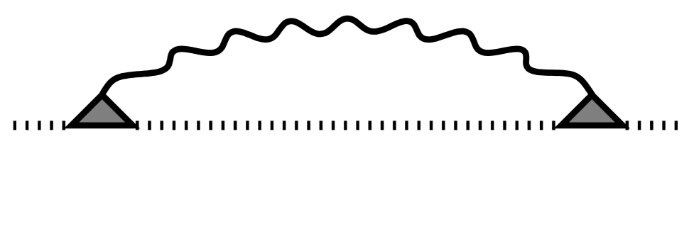
(c)

FIG. 4.: Magnon selfenergies describing the effect of magnon scattering on (a) orbital fluctuations, (b) charge fluctuations, and (c) phonons. Solid, dashed, dotted, and wiggled lines denote orbiton, holon, magnon, and phonon propagators, respectively.

An important piece of physics is still missed in the above treatment, namely the Jahn-Teller coupling of orbitals to the lattice.[21] In a cubic system there exist two independent Jahn-Teller modes $Q_{2}$ and $Q_{3}$ which lift the degeneracy of singly occupied $e_{g}$ orbitals. The interaction between orbitals and these two orthogonal lattice modes is described by

$$H_{\text{JT}}=-\sum_{i}\left(g_{2}Q_{2i}\sigma_{i}^{x}+g_{3}Q_{3i}\sigma^{z}_{i}\right),$$ (35)

where the Pauli matrices $\sigma^{x/z}_{i}$ act on the orbital subspace and the coupling constants $g_{2}\approx g_{3}$. The crystal dynamics is controlled by the Hamiltonian

$$H_{\text{ph}}=\frac{K}{2}\sum_{i}\mathchoice{{\hbox{\boldmath$\displaystyle Q$}}}{{\hbox{\boldmath$\textstyle Q$}}}{{\hbox{\boldmath$\scriptstyle Q$}}}{{\hbox{\boldmath$\scriptscriptstyle Q$}}}_{i}^{2}+K_{1}\sum_{\langle ij\rangle_{\gamma}}Q_{i}^{\gamma}Q_{j}^{\gamma}+\frac{1}{2M}\sum_{i}\mathchoice{{\hbox{\boldmath$\displaystyle P$}}}{{\hbox{\boldmath$\textstyle P$}}}{{\hbox{\boldmath$\scriptstyle P$}}}{{\hbox{\boldmath$\scriptscriptstyle P$}}}^{2}_{i},$$ (36)

with $Q_{i}^{x/y}=(Q_{3i}\pm\sqrt{3}Q_{2i})/2$, $Q_{i}^{z}=Q_{3i}$, and $\mathchoice{{\hbox{\boldmath$\displaystyle Q$}}}{{\hbox{\boldmath$\textstyle Q$}}}{{\hbox{\boldmath$\scriptstyle Q$}}}{{\hbox{\boldmath$\scriptscriptstyle Q$}}}_{i}=(Q_{2i},Q_{3i})$; $\mathchoice{{\hbox{\boldmath$\displaystyle P$}}}{{\hbox{\boldmath$\textstyle P$}}}{{\hbox{\boldmath$\scriptstyle P$}}}{{\hbox{\boldmath$\scriptscriptstyle P$}}}_{i}$ denotes the conjugate momentum vector corresponding to the lattice distortions $\mathchoice{{\hbox{\boldmath$\displaystyle Q$}}}{{\hbox{\boldmath$\textstyle Q$}}}{{\hbox{\boldmath$\scriptstyle Q$}}}{{\hbox{\boldmath$\scriptscriptstyle Q$}}}_{i}$. The three terms on the r.h.s. of Eq. (36) account for the crystal deformation energy, the correlations between neighboring sites, and the lattice kinetics, respectively. Equation (36) can be diagonalized in the momentum representation, yielding

$$H_{\text{ph}}=\sum_{\mathchoice{{\hbox{\boldmath$\displaystyle k$}}}{{\hbox{\boldmath$\textstyle k$}}}{{\hbox{\boldmath$\scriptstyle k$}}}{{\hbox{\boldmath$\scriptscriptstyle k$}}}\nu}\omega^{\nu}_{\mathchoice{{\hbox{\boldmath$\displaystyle k$}}}{{\hbox{\boldmath$\textstyle k$}}}{{\hbox{\boldmath$\scriptstyle k$}}}{{\hbox{\boldmath$\scriptscriptstyle k$}}}}a^{\dagger}_{\mathchoice{{\hbox{\boldmath$\displaystyle k$}}}{{\hbox{\boldmath$\textstyle k$}}}{{\hbox{\boldmath$\scriptstyle k$}}}{{\hbox{\boldmath$\scriptscriptstyle k$}}}\nu}a_{\mathchoice{{\hbox{\boldmath$\displaystyle k$}}}{{\hbox{\boldmath$\textstyle k$}}}{{\hbox{\boldmath$\scriptstyle k$}}}{{\hbox{\boldmath$\scriptscriptstyle k$}}}\nu},$$ (37)

with index $\nu=\pm$ and the phonon dispersions

$$\omega^{\pm}_{\mathchoice{{\hbox{\boldmath$\displaystyle k$}}}{{\hbox{\boldmath$\textstyle k$}}}{{\hbox{\boldmath$\scriptstyle k$}}}{{\hbox{\boldmath$\scriptscriptstyle k$}}}}=\omega_{0}\left(\kappa_{1\mathchoice{{\hbox{\boldmath$\displaystyle k$}}}{{\hbox{\boldmath$\textstyle k$}}}{{\hbox{\boldmath$\scriptstyle k$}}}{{\hbox{\boldmath$\scriptscriptstyle k$}}}}\pm\sqrt{\kappa_{2\mathchoice{{\hbox{\boldmath$\displaystyle k$}}}{{\hbox{\boldmath$\textstyle k$}}}{{\hbox{\boldmath$\scriptstyle k$}}}{{\hbox{\boldmath$\scriptscriptstyle k$}}}}^{2}+\kappa_{3\mathchoice{{\hbox{\boldmath$\displaystyle k$}}}{{\hbox{\boldmath$\textstyle k$}}}{{\hbox{\boldmath$\scriptstyle k$}}}{{\hbox{\boldmath$\scriptscriptstyle k$}}}}^{2}}\right)^{1/2}.$$ (38)

Here, $\kappa_{1\mathchoice{{\hbox{\boldmath$\displaystyle k$}}}{{\hbox{\boldmath$\textstyle k$}}}{{\hbox{\boldmath$\scriptstyle k$}}}{{\hbox{\boldmath$\scriptscriptstyle k$}}}}=1+k_{1}(c_{x}+c_{y}+c_{z})$, $\kappa_{2\mathchoice{{\hbox{\boldmath$\displaystyle k$}}}{{\hbox{\boldmath$\textstyle k$}}}{{\hbox{\boldmath$\scriptstyle k$}}}{{\hbox{\boldmath$\scriptscriptstyle k$}}}}=k_{1}\eta^{(2)}_{\mathchoice{{\hbox{\boldmath$\displaystyle k$}}}{{\hbox{\boldmath$\textstyle k$}}}{{\hbox{\boldmath$\scriptstyle k$}}}{{\hbox{\boldmath$\scriptscriptstyle k$}}}}$, $\kappa_{3\mathchoice{{\hbox{\boldmath$\displaystyle k$}}}{{\hbox{\boldmath$\textstyle k$}}}{{\hbox{\boldmath$\scriptstyle k$}}}{{\hbox{\boldmath$\scriptscriptstyle k$}}}}=k_{1}\eta^{(3)}_{\mathchoice{{\hbox{\boldmath$\displaystyle k$}}}{{\hbox{\boldmath$\textstyle k$}}}{{\hbox{\boldmath$\scriptstyle k$}}}{{\hbox{\boldmath$\scriptscriptstyle k$}}}}$ with $k_{1}=K_{1}/K$ and $\eta^{(2)}_{\mathchoice{{\hbox{\boldmath$\displaystyle k$}}}{{\hbox{\boldmath$\textstyle k$}}}{{\hbox{\boldmath$\scriptstyle k$}}}{{\hbox{\boldmath$\scriptscriptstyle k$}}}}=-\sqrt{3}(c_{x}-c_{y})/2$, $\eta^{(3)}_{\mathchoice{{\hbox{\boldmath$\displaystyle k$}}}{{\hbox{\boldmath$\textstyle k$}}}{{\hbox{\boldmath$\scriptstyle k$}}}{{\hbox{\boldmath$\scriptscriptstyle k$}}}}=c_{z}-\frac{1}{2}c_{x}-\frac{1}{2}c_{y}$ with $c_{\alpha}=\cos k_{\alpha}$, and $\omega_{0}=\sqrt{K/M}$.

While there is no direct coupling between spins and phonons in the present system, lattice modes nevertheless strongly affects the spin dynamics. The link between spin and lattice is established via the orbital channel: The coupling of orbitals to the lattice imposes low phononic frequencies onto orbital fluctuations. This acts to enhance the modulation of magnetic exchange bonds; thereby the effect of phonons extends onto the spin sector. To study this mechanism in more detail, we construct an effective spin-phonon-coupling Hamiltonian from which we then calculate the phononic contribution to the magnon selfenergy. Combining the spin-orbital-coupling term of the exchange Hamiltonians (18) and (LABEL:HJB) with the orbital-lattice Hamiltonian (35) we obtain (see Fig. 5):

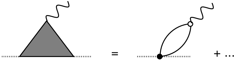
FIG. 5.: Effective spin-phonon-coupling vertex. The dominant contribution shown on the right stems from a combination of spin-orbital- (filled dot $\propto t$) and orbital-lattice- (open dot $\propto g_{2}$) coupling vertices. The orbital susceptibility depicted by a bubble controls the coupling strength. Solid, dotted, and wiggled lines represent orbiton, magnon, and phonon propagators, respectively.

$$H_{\text{s-ph}}=-\sum_{\mathchoice{{\hbox{\boldmath$\displaystyle p$}}}{{\hbox{\boldmath$\textstyle p$}}}{{\hbox{\boldmath$\scriptstyle p$}}}{{\hbox{\boldmath$\scriptscriptstyle p$}}}\mathchoice{{\hbox{\boldmath$\displaystyle q$}}}{{\hbox{\boldmath$\textstyle q$}}}{{\hbox{\boldmath$\scriptstyle q$}}}{{\hbox{\boldmath$\scriptscriptstyle q$}}}\nu}g_{\mathchoice{{\hbox{\boldmath$\displaystyle p$}}}{{\hbox{\boldmath$\textstyle p$}}}{{\hbox{\boldmath$\scriptstyle p$}}}{{\hbox{\boldmath$\scriptscriptstyle p$}}}\mathchoice{{\hbox{\boldmath$\displaystyle q$}}}{{\hbox{\boldmath$\textstyle q$}}}{{\hbox{\boldmath$\scriptstyle q$}}}{{\hbox{\boldmath$\scriptscriptstyle q$}}}}^{\nu}(a^{\dagger}_{\mathchoice{{\hbox{\boldmath$\displaystyle q$}}}{{\hbox{\boldmath$\textstyle q$}}}{{\hbox{\boldmath$\scriptstyle q$}}}{{\hbox{\boldmath$\scriptscriptstyle q$}}}\nu}+a_{\mathchoice{{\hbox{\boldmath$\displaystyle q$}}}{{\hbox{\boldmath$\textstyle q$}}}{{\hbox{\boldmath$\scriptstyle q$}}}{{\hbox{\boldmath$\scriptscriptstyle q$}}}\nu})B^{\dagger}_{\mathchoice{{\hbox{\boldmath$\displaystyle p$}}}{{\hbox{\boldmath$\textstyle p$}}}{{\hbox{\boldmath$\scriptstyle p$}}}{{\hbox{\boldmath$\scriptscriptstyle p$}}}}B_{\mathchoice{{\hbox{\boldmath$\displaystyle p$}}}{{\hbox{\boldmath$\textstyle p$}}}{{\hbox{\boldmath$\scriptstyle p$}}}{{\hbox{\boldmath$\scriptscriptstyle p$}}}+\mathchoice{{\hbox{\boldmath$\displaystyle q$}}}{{\hbox{\boldmath$\textstyle q$}}}{{\hbox{\boldmath$\scriptstyle q$}}}{{\hbox{\boldmath$\scriptscriptstyle q$}}}}.$$ (39)

The coupling constants in Eq. (39) are

$$g_{\mathchoice{{\hbox{\boldmath$\displaystyle p$}}}{{\hbox{\boldmath$\textstyle p$}}}{{\hbox{\boldmath$\scriptstyle p$}}}{{\hbox{\boldmath$\scriptscriptstyle p$}}}\mathchoice{{\hbox{\boldmath$\displaystyle q$}}}{{\hbox{\boldmath$\textstyle q$}}}{{\hbox{\boldmath$\scriptstyle q$}}}{{\hbox{\boldmath$\scriptscriptstyle q$}}}}^{+} = \epsilon_{0}\left(\frac{\omega_{0}}{\omega_{\mathchoice{{\hbox{\boldmath$\displaystyle q$}}}{{\hbox{\boldmath$\textstyle q$}}}{{\hbox{\boldmath$\scriptstyle q$}}}{{\hbox{\boldmath$\scriptscriptstyle q$}}}}^{+}}\right)^{1/2}\left(\lambda_{\mathchoice{{\hbox{\boldmath$\displaystyle p$}}}{{\hbox{\boldmath$\textstyle p$}}}{{\hbox{\boldmath$\scriptstyle p$}}}{{\hbox{\boldmath$\scriptscriptstyle p$}}}\mathchoice{{\hbox{\boldmath$\displaystyle q$}}}{{\hbox{\boldmath$\textstyle q$}}}{{\hbox{\boldmath$\scriptstyle q$}}}{{\hbox{\boldmath$\scriptscriptstyle q$}}}}^{(3)}\cos\Theta_{\mathchoice{{\hbox{\boldmath$\displaystyle q$}}}{{\hbox{\boldmath$\textstyle q$}}}{{\hbox{\boldmath$\scriptstyle q$}}}{{\hbox{\boldmath$\scriptscriptstyle q$}}}}-\lambda_{\mathchoice{{\hbox{\boldmath$\displaystyle p$}}}{{\hbox{\boldmath$\textstyle p$}}}{{\hbox{\boldmath$\scriptstyle p$}}}{{\hbox{\boldmath$\scriptscriptstyle p$}}}\mathchoice{{\hbox{\boldmath$\displaystyle q$}}}{{\hbox{\boldmath$\textstyle q$}}}{{\hbox{\boldmath$\scriptstyle q$}}}{{\hbox{\boldmath$\scriptscriptstyle q$}}}}^{(2)}\sin\Theta_{\mathchoice{{\hbox{\boldmath$\displaystyle q$}}}{{\hbox{\boldmath$\textstyle q$}}}{{\hbox{\boldmath$\scriptstyle q$}}}{{\hbox{\boldmath$\scriptscriptstyle q$}}}}\right),$$

$$g_{\mathchoice{{\hbox{\boldmath$\displaystyle p$}}}{{\hbox{\boldmath$\textstyle p$}}}{{\hbox{\boldmath$\scriptstyle p$}}}{{\hbox{\boldmath$\scriptscriptstyle p$}}}\mathchoice{{\hbox{\boldmath$\displaystyle q$}}}{{\hbox{\boldmath$\textstyle q$}}}{{\hbox{\boldmath$\scriptstyle q$}}}{{\hbox{\boldmath$\scriptscriptstyle q$}}}}^{-} = \epsilon_{0}\left(\frac{\omega_{0}}{\omega_{\mathchoice{{\hbox{\boldmath$\displaystyle q$}}}{{\hbox{\boldmath$\textstyle q$}}}{{\hbox{\boldmath$\scriptstyle q$}}}{{\hbox{\boldmath$\scriptscriptstyle q$}}}}^{-}}\right)^{1/2}\left(\lambda_{\mathchoice{{\hbox{\boldmath$\displaystyle p$}}}{{\hbox{\boldmath$\textstyle p$}}}{{\hbox{\boldmath$\scriptstyle p$}}}{{\hbox{\boldmath$\scriptscriptstyle p$}}}\mathchoice{{\hbox{\boldmath$\displaystyle q$}}}{{\hbox{\boldmath$\textstyle q$}}}{{\hbox{\boldmath$\scriptstyle q$}}}{{\hbox{\boldmath$\scriptscriptstyle q$}}}}^{(3)}\sin\Theta_{\mathchoice{{\hbox{\boldmath$\displaystyle q$}}}{{\hbox{\boldmath$\textstyle q$}}}{{\hbox{\boldmath$\scriptstyle q$}}}{{\hbox{\boldmath$\scriptscriptstyle q$}}}}+\lambda_{\mathchoice{{\hbox{\boldmath$\displaystyle p$}}}{{\hbox{\boldmath$\textstyle p$}}}{{\hbox{\boldmath$\scriptstyle p$}}}{{\hbox{\boldmath$\scriptscriptstyle p$}}}\mathchoice{{\hbox{\boldmath$\displaystyle q$}}}{{\hbox{\boldmath$\textstyle q$}}}{{\hbox{\boldmath$\scriptstyle q$}}}{{\hbox{\boldmath$\scriptscriptstyle q$}}}}^{(2)}\cos\Theta_{\mathchoice{{\hbox{\boldmath$\displaystyle q$}}}{{\hbox{\boldmath$\textstyle q$}}}{{\hbox{\boldmath$\scriptstyle q$}}}{{\hbox{\boldmath$\scriptscriptstyle q$}}}}\right),$$

with $\epsilon_{0}=(E_{\text{JT}}a_{0}^{2}\omega_{0}/S^{2})^{1/2}$ and $\lambda^{(\alpha)}_{\mathchoice{{\hbox{\boldmath$\displaystyle p$}}}{{\hbox{\boldmath$\textstyle p$}}}{{\hbox{\boldmath$\scriptstyle p$}}}{{\hbox{\boldmath$\scriptscriptstyle p$}}}\mathchoice{{\hbox{\boldmath$\displaystyle q$}}}{{\hbox{\boldmath$\textstyle q$}}}{{\hbox{\boldmath$\scriptstyle q$}}}{{\hbox{\boldmath$\scriptscriptstyle q$}}}}=(\eta^{(\alpha)}_{\mathchoice{{\hbox{\boldmath$\displaystyle q$}}}{{\hbox{\boldmath$\textstyle q$}}}{{\hbox{\boldmath$\scriptstyle q$}}}{{\hbox{\boldmath$\scriptscriptstyle q$}}}}-\eta^{(\alpha)}_{\mathchoice{{\hbox{\boldmath$\displaystyle p$}}}{{\hbox{\boldmath$\textstyle p$}}}{{\hbox{\boldmath$\scriptstyle p$}}}{{\hbox{\boldmath$\scriptscriptstyle p$}}}}-\eta^{(\alpha)}_{\mathchoice{{\hbox{\boldmath$\displaystyle p$}}}{{\hbox{\boldmath$\textstyle p$}}}{{\hbox{\boldmath$\scriptstyle p$}}}{{\hbox{\boldmath$\scriptscriptstyle p$}}}+\mathchoice{{\hbox{\boldmath$\displaystyle q$}}}{{\hbox{\boldmath$\textstyle q$}}}{{\hbox{\boldmath$\scriptstyle q$}}}{{\hbox{\boldmath$\scriptscriptstyle q$}}}})$. Further

$$\cos\Theta_{\mathchoice{{\hbox{\boldmath$\displaystyle q$}}}{{\hbox{\boldmath$\textstyle q$}}}{{\hbox{\boldmath$\scriptstyle q$}}}{{\hbox{\boldmath$\scriptscriptstyle q$}}}} = \frac{1}{\sqrt{2}}\left(1+\frac{\kappa_{3\mathchoice{{\hbox{\boldmath$\displaystyle q$}}}{{\hbox{\boldmath$\textstyle q$}}}{{\hbox{\boldmath$\scriptstyle q$}}}{{\hbox{\boldmath$\scriptscriptstyle q$}}}}}{\sqrt{\kappa_{2\mathchoice{{\hbox{\boldmath$\displaystyle q$}}}{{\hbox{\boldmath$\textstyle q$}}}{{\hbox{\boldmath$\scriptstyle q$}}}{{\hbox{\boldmath$\scriptscriptstyle q$}}}}^{2}+\kappa_{3\mathchoice{{\hbox{\boldmath$\displaystyle q$}}}{{\hbox{\boldmath$\textstyle q$}}}{{\hbox{\boldmath$\scriptstyle q$}}}{{\hbox{\boldmath$\scriptscriptstyle q$}}}}^{2}}}\right)^{1/2},$$

$$\sin\Theta_{\mathchoice{{\hbox{\boldmath$\displaystyle q$}}}{{\hbox{\boldmath$\textstyle q$}}}{{\hbox{\boldmath$\scriptstyle q$}}}{{\hbox{\boldmath$\scriptscriptstyle q$}}}} = \frac{1}{\sqrt{2}}\left(1-\frac{\kappa_{3\mathchoice{{\hbox{\boldmath$\displaystyle q$}}}{{\hbox{\boldmath$\textstyle q$}}}{{\hbox{\boldmath$\scriptstyle q$}}}{{\hbox{\boldmath$\scriptscriptstyle q$}}}}}{\sqrt{\kappa_{2\mathchoice{{\hbox{\boldmath$\displaystyle q$}}}{{\hbox{\boldmath$\textstyle q$}}}{{\hbox{\boldmath$\scriptstyle q$}}}{{\hbox{\boldmath$\scriptscriptstyle q$}}}}^{2}+\kappa_{3\mathchoice{{\hbox{\boldmath$\displaystyle q$}}}{{\hbox{\boldmath$\textstyle q$}}}{{\hbox{\boldmath$\scriptstyle q$}}}{{\hbox{\boldmath$\scriptscriptstyle q$}}}}^{2}}}\right)^{1/2}\text{sign}(\kappa_{2\mathchoice{{\hbox{\boldmath$\displaystyle q$}}}{{\hbox{\boldmath$\textstyle q$}}}{{\hbox{\boldmath$\scriptstyle q$}}}{{\hbox{\boldmath$\scriptscriptstyle q$}}}}).$$

The strength of the spin-lattice interaction is controlled by the orbital susceptibility $\langle(f^{\dagger}_{i+z,\uparrow}f_{i\uparrow})(\sigma_{i}^{z})\rangle_{\omega}$ which enters the parameter $a_{0}=t(x+x_{0})\langle(f^{\dagger}_{i+z,\uparrow}f_{i\uparrow})(\sigma_{i}^{z})\rangle_{\omega=0}$; the zero-frequency limit is admissible bearing in mind that the energy scale of orbital fluctuations exceeds the one of phonons. The phononic contribution to the magnon selfenergy that follows from Hamiltonian (39) can finally be calculated, the corresponding diagram is depicted in Fig. 4(c).

IV Comparison with Experiment

We are now in the position to evaluate the selfenergies of Fig. 4. Charge and orbital susceptibilities are calculated using mean-field Green’s functions in slave-boson $h_{i}$ and fermion $f_{i}$ subspaces. For the spectral density of Jahn-Teller phonons in Fig. 4(c) we employ the expression

$$\rho^{\text{ph}}_{\pm}(\omega,\mathchoice{{\hbox{\boldmath$\displaystyle q$}}}{{\hbox{\boldmath$\textstyle q$}}}{{\hbox{\boldmath$\scriptstyle q$}}}{{\hbox{\boldmath$\scriptscriptstyle q$}}})=\frac{1}{\pi}\frac{\omega}{\omega_{\mathchoice{{\hbox{\boldmath$\displaystyle q$}}}{{\hbox{\boldmath$\textstyle q$}}}{{\hbox{\boldmath$\scriptstyle q$}}}{{\hbox{\boldmath$\scriptscriptstyle q$}}}}^{\pm}}\frac{\Gamma}{(\omega-\omega_{\mathchoice{{\hbox{\boldmath$\displaystyle q$}}}{{\hbox{\boldmath$\textstyle q$}}}{{\hbox{\boldmath$\scriptstyle q$}}}{{\hbox{\boldmath$\scriptscriptstyle q$}}}}^{\pm})^{2}+\Gamma^{2}},$$ (40)

which phenomenologically accounts for the damping $\Gamma$ of phonons due to their coupling to orbital fluctuations. The phonon dispersion $\omega_{\mathchoice{{\hbox{\boldmath$\displaystyle q$}}}{{\hbox{\boldmath$\textstyle q$}}}{{\hbox{\boldmath$\scriptstyle q$}}}{{\hbox{\boldmath$\scriptscriptstyle q$}}}}^{\pm}$ is given by Eq. (38).

The expressions obtained from the diagrams in Fig. 4 contain summations over momentum space which we perform numerically using a Monte-Carlo algorithm. The result is shown by solid lines in Fig. 6.

FIG. 6.: Magnon dispersion along $(0,0,\xi)$, $(\xi,\xi,0)$, and $(\xi,\xi,\xi)$ directions, where $\xi=0.5$ at the cubic zone boundary. Experimental data from Ref. [8] are indicated by circles, the mean-field dispersion $\omega_{\mathchoice{{\hbox{\boldmath$\displaystyle p$}}}{{\hbox{\boldmath$\textstyle p$}}}{{\hbox{\boldmath$\scriptstyle p$}}}{{\hbox{\boldmath$\scriptscriptstyle p$}}}}$ of Eq. (29) is marked by a dashed line; the latter is of conventional nearest-neighbor Heisenberg form. Solid lines represent the theoretical result for the dispersion $\tilde{\omega}_{\mathchoice{{\hbox{\boldmath$\displaystyle p$}}}{{\hbox{\boldmath$\textstyle p$}}}{{\hbox{\boldmath$\scriptstyle p$}}}{{\hbox{\boldmath$\scriptscriptstyle p$}}}}$ defined by Eq. (26); it includes charge, orbital, and lattice effects. The upper curve is obtained for dispersionless phonons with $k_{1}=0$, the lower one is a fit to the experimental data with $k_{1}=-0.33$ corresponding to ferrotype orbital-lattice correlations.

For comparison, the experimental data of Ref. [8] are marked by circles and the bare mean-field dispersion $\omega_{\mathchoice{{\hbox{\boldmath$\displaystyle p$}}}{{\hbox{\boldmath$\textstyle p$}}}{{\hbox{\boldmath$\scriptstyle p$}}}{{\hbox{\boldmath$\scriptscriptstyle p$}}}}$ is indicated by a dashed line. The following parameters are chosen: The hopping amplitude $t=0.4$ eV is adjusted to fit the spin stiffness in Pr_0.63Sr_0.37MnO₃;[8] further we use $U_{1}=4$ eV.[14] The phonon contribution depends on the quantities $E_{\text{JT}}a_{0}^{2}\equiv(g_{2}a_{0})^{2}/2K=0.004$ eV,[22] $\omega_{0}=0.08$ eV,[23] and $\Gamma=0.04$ eV.

The upper solid line in Fig. 6 is obtained for $k_{1}=0$. In this case intersite orbital-lattice correlations in Hamiltonian (36) are discarded — phonons are dispersionless. A pronounced softening of magnons at large momenta can be observed. A more detailed analysis reveals this effect to be mostly due to fluctuations of the orbital and lattice degrees of freedom. In contrast, charge fluctuations are found to play only a minor role. We attribute this to the fact that the spectral density of charge fluctuations lies well above the magnon band. Orbital and lattice fluctuations, on the other hand, are of rather low frequency ($\propto xt$ and $\propto\omega_{0}^{\text{ph}}$, respectively) and hence affect the spin-wave dispersion in a more pronounced way.

The lower solid line in Fig. 6 is obtained for $k_{1}=-0.33$ which yields a fit to the experimental data of Ref. [8]. The directional dependence of the magnon renormalization seen in experiment is well reproduced: The effect is strongest in $(0,0,\xi)$ and $(0,\xi,\xi)$ directions. A key observation here is the crucial role of intersite correlations of orbital-lattice distortions — these are captured by the phononic dispersion being controlled by the parameter $k_{1}$. In order to reproduce the experimental data we are forced to assume these correlations to be of ferrotype, i.e., $k_{1}<0$. We believe this somewhat surprising result to reflect an important piece of new physics: Conventionally one would expect $k_{1}>0$ associated with a tendency of the orbital/lattice sector to develop antiferrotype order.[13] In the hole-doped system, however, this effect competes against charge mobility which prefers a ferrotype orbital orientation. The latter allows to minimize the kinetic energy by maximizing the transfer amplitude between sites. While Jahn-Teller lattice effects prevail at low doping, we speculate the kinetic energy to dominate at large enough hole concentrations. In fact, low-dimensional ferrotype orbital correlations (resonating $|x^{2}-y^{2}\rangle$, $|x^{2}-z^{2}\rangle$, $|y^{2}-z^{2}\rangle$ planar configurations) have been observed to evolve in a bosonic description of orbital fluctuations.[10] The fermionic description of orbitals employed in the present work emphasizes on modeling a strongly fluctuating orbital-liquid state, but underestimates these orbital-lattice instabilities. In order to simulate the competition between Jahn-Teller effect and kinetic energy we therefore turn to a phenomenological approach: By tuning the parameter $k_{1}$ we control the character of intersite orbital-lattice correlations. The result for different values of $k_{1}$ is shown in Fig. 7 where $E_{\text{JT}}a_{0}^{2}=0.006$ eV is used.

FIG. 7.: Magnon dispersion including charge, orbital, and lattice effects. Different values for $k_{1}$ controlling intersite orbital-lattice correlations are used. The softening enhances as $k_{1}\rightarrow-\frac{1}{3}$ corresponding to an instability point towards ferrotype orbital-lattice order.

Ferrotype orbital correlations with $k_{1}<0$ are found to be most effective in renormalizing the magnon spectrum. This is ascribed to slowly fluctuating layered orbital configurations which effectively reduce the dimensionality of exchange bonds. We note that magnons in $(\xi,\xi,\xi)$ direction are sensible to all three spatial directions of the exchange bonds; their dispersion therefore remains unaffected by the local symmetry breaking induced by low-dimensional orbital correlations. As an instability towards orbital-lattice order is approached, exchange-bond fluctuations become quasistatic. In the magnon spectrum this is reflected by a strong enhancement of the renormalization effect as is seen in Fig. 7 for $k_{1}\rightarrow-\frac{1}{3}$. The layered orbital structure which evolves at this point is accompanied by a layered spin structure; the latter is indeed experimentally observed at doping levels of about $x=0.5$.[24, 25]

We finally note that the softening of magnons at the zone boundary leads to a reduction of $T_{C}$. Remarkably, the small-$q$ spin stiffness $D$ remains unaffected which explains the anomalous enhancement of the $D/T_{C}$ ratio in low-$T_{C}$ manganites.[9]

V Conclusion

In summary, we have presented a theory of the spin dynamics in ferromagnetic manganites. Taking into account the orbital degeneracy and the correlated nature of $e_{g}$ electrons, we analyzed the structure of magnetic exchange bonds; these are established by the intersite transfer of electrons in coherent double-exchange and virtual superexchange processes. Orbital and charge fluctuations are shown to strongly modulate the exchange bonds, leading to a softening of the magnon excitation spectrum close to the Brillouin zone boundary. The presence of Jahn-Teller phonons further enhances the effect. This peculiar interplay between double-exchange physics and orbital-lattice dynamics becomes dominant close to the instability towards an orbital-lattice ordered state. The unusual magnon dispersion experimentally observed in low-$T_{C}$ manganites can hence be understood as a precursor effect of orbital-lattice ordering. While the softening of magnons at the zone boundary is responsible for reducing the value of $T_{C}$, the small-momentum spin dynamics that enters the spin-wave stiffness $D$ remains virtually unaffected. This explains the enhancement of the ratio $D/T_{C}$ observed in low-$T_{C}$ compounds. In general it can be concluded that strong correlations and orbital fluctuations play a crucial role in explaining the peculiar magnetic properties of metallic manganites.

We would like to thank H. Y. Hwang and P. Horsch for stimulating discussions.

REFERENCES

• [1] Permanent address: Kazan Physicotechnical Institute, 420029 Kazan, Russia.
• [2] C. Zener, Phys. Rev. 82, 403 (1951).
• [3] P. W. Anderson and H. Hasegawa, Phys. Rev. 100, 675 (1955).
• [4] P.-G. de Gennes, Phys. Rev. 118, 141 (1960).
• [5] K. Kubo and N. Ohata, J. Phys. Soc. Jpn. 33, 21 (1972).
• [6] N. Furukawa, J. Phys. Soc. Jpn. 65, 1174 (1996).
• [7] T. G. Perring, G. Aeppli, S. M. Hayden, S. A. Carter, J. P. Remeika, and S.-W. Cheong, Phys. Rev. Lett. 77, 711 (1996).
• [8] H. Y. Hwang, P. Dai, S.-W. Cheong, G. Aeppli, D. A. Tennant, and H. A. Mook, Phys. Rev. Lett. 80, 1316 (1998).
• [9] J. A. Fernandez-Baca, P. Dai, H. Y. Hwang, C. Kloc, and S.-W. Cheong, Phys. Rev. Lett. 80, 4012 (1998).
• [10] S. Ishihara, M. Yamanaka, and N. Nagaosa, Phys. Rev. B 56, 686 (1997).
• [11] R. Kilian and G. Khaliullin, Phys. Rev. B 58, R11 841 (1998).
• [12] N. Furukawa, cond-mat/9905133 (unpublished).
• [13] K. I. Kugel and D. I. Khomskii, Sov. Phys. Usp. 25, 231 (1982).
• [14] L. F. Feiner and A. M. Oleś, Phys. Rev. B 59, 3295 (1999).
• [15] A. Auerbach, Interacting Electrons and Quantum Magnetism (Springer-Verlag, New York, 1994).
• [16] It is noticed that the phase-dependent part of the fermionic hopping is only of order $1/S$ [see Eq. (18)].
• [17] A. J. Millis, P. B. Littlewood, and B. I. Shraiman, Phys. Rev. Lett. 74, 5144 (1995).
• [18] E. Müller-Hartmann and E. Dagotto, Phys. Rev. B 54, R6819 (1996).
• [19] Here we do not discuss the superexchange between core spins as well as finite-$J_{H}$ effects which are responsible for a variety of antiferromagnetic structures in manganites. These effects are only of minor importance in the cubic metallic phase under consideration.
• [20] The effect of superexchange-bond fluctuations on the magnon spectrum in the antiferromagnetic Kugel-Khomskii model was recently studied in G. Khaliullin and V. Oudovenko, Phys. Rev. B 56, R14 243 (1997).
• [21] A. J. Millis, B. Shraiman, and R. Mueller, Phys. Rev. Lett. 77, 175 (1996).
• [22] A mean-field calculation gives $a_{0}\approx 0.1$. Our fitting then implies a reasonable Jahn-Teller binding energy $E_{\text{JT}}\approx 0.4$ eV.
• [23] This number is consistent with optical reflectivity data in Y. Okimoto, T. Katsufuji, T. Ishikawa, A. Urushibara, T. Arima, and Y. Tokura, Phys. Rev. Lett. 75, 109 (1995).
• [24] H. Kawano, R. Kajimoto, H. Yoshizawa, Y. Tomioka, H. Kuwahara, and Y. Tokura, Phys. Rev. Lett. 78, 4253 (1997).
• [25] Y. Moritomo, T. Akimoto, A. Nakamura, K. Ohoyama, and M. Ohashi, Phys. Rev. B 58, 5544 (1998).