High-Acceleration Patterns in Thin Vibrated Granular Layers

Abstract

Theoretical and experimental study of high-acceleration patterns in vibrated granular layers is presented. The order parameter model based on parametric Ginzburg-Landau equation is used to describe strongly nonlinear excitations including hexagons, interface between flat anti-phase domains and new localized objects, super-oscillons. The experiments confirmed the existence of super-oscillons and bound states of super-oscillons and interfaces. On the basis of order parameter model we predict analytically and confirm experimentally that the additional subharmonic driving results in controlled motion of the interfaces.

The collective dynamics of granular materials is a subject of current interest [1, 2, 3, 4, 5]. The intrinsic dissipative nature of the interactions between the constituent macroscopic particles give rise to several basic properties specific to granular substances and setting granular matter apart from the conventional gaseous, liquid, or solid states.

Driven granular systems manifest collective fluid-like behavior: convection, surface waves, and pattern formation (see e.g. [1]). One of the most fascinating examples of this collective dynamics is the appearance of long-range coherent patterns and localized excitations in vertically-vibrated thin granular layers [2, 3, 4, 5, 6, 7]. The particular pattern is determined by the interplay between driving frequency $f$ and acceleration of the container $\Gamma=4\pi^{2}{\cal A}f^{2}/g$ (${\cal A}$ is the amplitude of oscillations, $g$ is the gravity acceleration) [2, 3].

Patterns appear at $\Gamma\approx 2.4$ almost independently of the driving frequency $f$. At small frequencies $f<f^{*}$ [3, 4] the transition is subcritical (hysteretic), leading to formation of squares. In the hysteretic region, localized excitations such as individual oscillons and various bound states of oscillons appear as $\Gamma$ is decreased. For higher frequencies $f>f^{*}$ the onset pattern is stripes, and at the frequency slightly higher than $f^{*}$ the transition becomes supercritical. Both squares and stripes, as well as oscillons, oscillate at half of the driving frequency $f/2$. At higher acceleration ($\Gamma>4$), stripes and squares become unstable, and hexagons appear instead. Further increase of acceleration at $\Gamma\approx 4.5$ converts hexagons into a domain-like structure of flat layers oscillating with frequency $f/2$ with opposite phases. Depending on parameters, interfaces separating flat domains, are either smooth or ”decorated” by periodic undulations. For $\Gamma>5.7$ various quarter-harmonic patters emerge.

The pattern formation in thin layers of granular material was studied theoretically by several groups. Direct molecular dynamics simulations [8, 9] (see also [10]) reproduced a majority of patterns observed in experiments and many features of the bifurcation diagram, although until now have not yielded oscillons and interfaces. Hydrodynamic and phenomenological models [11, 12] reproduced certain experimental features, however neither of them offered a systematic description of the whole rich variety of the observed phenomena. In Refs. [13, 14] we introduced the order parameter characterizing the complex amplitude of sub-harmonic oscillations. The equations of motion following from the symmetry arguments and mass conservation reproduced essential phenomenology of patterns near the threshold of primary bifurcation: stripes, squares, and, localized objects, oscillons.

In this paper we describe high acceleration patterns on the basis of the same order parameter model and compare it with experimental observations. Our preliminary results were published earlier in Refs. [5, 14, 15]. Here we show that at large amplitude of driving both hexagons and interfaces emerge. We find morphological instability leading to the formation of “decorated” interfaces. We study the motion of the interface under the influence of a small subharmonic component in the driving acceleration. We also find a new localized structure, ”super-oscillon”, which exists for high acceleration values. We discuss possible mechanisms of saturation of the interface instability. Our experimental results demonstrate the existence of super-oscillons and bound states of super-oscillons and interfaces. They also confirm theoretical predictions of the externally controlled interface motion.

The structure of the article is following. In Sec. I we introduce our phenomenological order-parameter model. In Sec. II we develop the weakly-nonlinear theory for the flat period-doubled state of the vibrated layer. In Sec. III we analyze the interface solution and study its stability with respect to transverse perturbations. In Sec. IV we discuss new localized solutions. In Sec. V we present the combined theoretical phase diagram of the model. In Sec. VI we demonstrate that in a certain limit our model can be reduced to the real Swift-Hohenberg equation. This equation also possesses a similar variety of patterns including stripes, hexagons, stable and unstable interface solutions, as well as localized solutions. In Sec. VII we demonstrate that additional subharmonic driving results in drift of the interface with the velocity determined by the amplitude of the driving and the direction determined by the relative phase. In Sec. VIII we present our experimental results. It includes the study phase diagram and the effect of additional subharmonic driving. Section IX summarizes our conclusions.

I Parametric Ginzburg-Landau Equation

The essence of the model [13, 14] is the order parameter equation for the complex amplitude $\psi$ of parametric layer oscillations $h=\psi\exp(i\pi ft)+c.c.$ at the frequency $f/2$ coupled with the equation for the thickness of the layer $\rho$ averaged over the period of vibrations,

$$\partial_{t}\psi = \gamma\psi^{*}-(1-i\omega)\psi+(1+ib)\nabla^{2}\psi-|\psi|^{2}\psi-\rho\psi$$ (1)

$$\partial_{t}\rho = \zeta\nabla\cdot(\rho\nabla|\psi|^{2})+\beta\nabla^{2}\rho$$ (2)

Here $\gamma$ is the normalized amplitude of forcing at the resonant frequency $f$. Linear terms in Eq. (1) can be obtained from the complex growth rate for infinitesimal periodic layer perturbations $h\sim\exp[\Lambda(k)t+ikx]$. Expanding $\Lambda(k)$ for small $k$, and keeping only two leading terms in the expansion $\Lambda(k)=-\Lambda_{0}-\Lambda_{1}k^{2}$ we obtain the linear terms in Eq. (1), where $b=Im\Lambda_{1}/Re\Lambda_{1}$ characterizes ratio of dispersion to diffusion and parameter $\omega=(\Omega_{0}-\pi f)/Re\Lambda_{0}$, $\Omega_{0}=-Im\Lambda_{0}$ characterizes the frequency of the driving. In Eq. (2) $\zeta,\beta$ are transport coefficients for $\rho$. Slowly-varying thickness of the layer $\rho$ controls the dissipation rate (the last term in Eq.(1)). The second equation (2) describes re-distribution of the averaged thickness due to the diffusive flux $\propto-\nabla\rho$, and an additional flux $\propto-\rho\nabla|\psi|^{2}$ caused by the spatially nonuniform vibrations of the granular material. This coupled model was used in Refs.[13, 14] to describe the pattern selection near the threshold of the primary bifurcation. It was shown that at small $\zeta\rho_{0}\beta^{-1}$ (which corresponds to low frequencies and thick layers), the primary bifurcation is subcritical and leads to the emergence of square patterns. For higher frequencies and/or thinner layers, transition is supercritical and leads to roll patterns. At intermediate frequencies ($f\approx f^{*}$), the stable localized solutions of Eqs.(1),(2) corresponding to isolated oscillons and variety of bound states were found in agreement with experiment.

In this paper we focus on high-acceleration patterns at high frequencies. In Ref. [13] it was indicated that the density transport coefficient $\beta$ is proportional to the energy of plate vibration ($\propto f^{2}$), and, therefore, it should increase with the driving frequency $f$. As a result, for high frequencies the coupling between $\rho$ and $\psi$ becomes less relevant, and one can assume $\rho=$const and exclude it from Eq.(1) by rescaling. Then the model can be reduced to a single order-parameter equation

$$\partial_{t}\psi = \gamma\psi^{*}-(1-i\omega)\psi+(1+ib)\nabla^{2}\psi-|\psi|^{2}\psi$$ (3)

Eq.(3) also describes the evolution of the order parameter for the parametric instability in vertically oscillating fluid layers (see [17, 18]).

It is convenient to shift the phase of the complex order parameter via $\tilde{\psi}=\psi\exp(i\phi)$ with $\sin 2\phi=\omega/\gamma$. The equations for real and imaginary part $\tilde{\psi}=A+iB$ are:

$$\partial_{t}A = (s-1)A-2\omega B-(A^{2}+B^{2})A+\nabla^{2}(A-bB)$$ (4)

$$\partial_{t}B = -(s+1)B-(A^{2}+B^{2})B+\nabla^{2}(B+bA)$$ (5)

where $s^{2}=\gamma^{2}-\omega^{2}$.

II Stability of uniform states

At $s<1$, Eqs. (4),(5) has only one trivial uniform state $A=0,\ B=0$, At $s>1$, two new uniform states appear, $A=\pm\sqrt{s-1},B=0$. The onset of these states corresponds to the period doubling of the layer flights sequence, observed in experiments [2] and predicted by the simple inelastic ball model [2, 19]. Signs $\pm$ reflect two relative phases of layer flights with respect to container vibrations[16].

The trivial flat state $A=B=0$ loses stability if the following condition fulfilled (compare [13]):

$$\gamma^{2}>\frac{(\omega+b)^{2}}{1+b^{2}}$$ (6)

Because of the symmetry of Eq.(3), small perturbations from the trivial state lead to the formation of a periodic sequence of rolls or stripes.

Let us analyze the stability of the non-trivial states $A=\pm\sqrt{s-1},B=0$ with respect to small perturbations with wavenumber $k$

$${A\choose B}={\pm\sqrt{s-1}\choose 0}+{U_{k}\choose V_{k}}\exp[\lambda(k)t+ikx].$$ (7)

At the threshold the uniform state loses its stability with respect to periodic modulations with the critical wavenumber $k_{c}$ at $s<s_{c}$ (correspondingly, $\gamma<\gamma_{c}$), where

$$s_{c} = \frac{\sqrt{(1+\omega^{2})(1+b^{2})}-\omega+b}{2b}$$ (8)

$$k_{c}^{2} = -\frac{2s-1-\omega b}{1+b^{2}}$$ (9)

Small perturbations with every direction of the wavevector grow at the same rate. The resultant selected pattern is determined by the nonlinear competition between the modes. In the presence of the reflection symmetry $\psi\to-\psi$, quadratic nonlinearity is absent, and cubic nonlinearity near the trivial state favors stripes corresponding to a single mode. Near the fixed points $A=\pm\sqrt{s-1},B=0$ the reflection symmetry for perturbations $U\to-U,\ V\to-V$ is broken, and hexagons emerge at the threshold of the instability. To clarify this point we perform weakly-nonlinear analysis of Eqs. (4),(5) for $s=s_{c}-\epsilon$, and $\epsilon\ll 1$. At $\epsilon\to 0$, the variables $U$ and $V$ are related as in linear system:

$${U\choose V} = {1\choose\eta}\Psi$$ (10)

$$\Psi = \sum A_{j}\exp[i{\bf kr}]+c.c.,$$ (11)

where $|k|=k_{c}$ and $\eta=\left[2(s_{c}-1)+k^{2}_{c}\right]/(bk^{2}_{c}-2\omega)$.

Corresponding adjoint eigenvector is

$${U^{+}\choose V^{+}}={1\choose\eta^{+}}$$ (12)

where $\eta^{+}=-\left[2(s_{c}-1)+k^{2}_{c}\right]/bk^{2}_{c}$. Substituting Eq. (11) into Eqs. (4),(5) and performing the orthogonalization, we obtain equations for the slowly-varying complex amplitudes $A_{j}$, $j=1,2,3$ (we assume only three waves with triangular symmetry, favored by quadratic nonlinearity)

$$\partial_{t}A_{j} = 2\epsilon A_{j}+a_{2}A_{j+1}^{*}A_{j-1}^{*}$$ (13)

$$- a_{3}\left(|A_{j}|^{2}+2(|A_{j-1}|^{2}+|A_{j+1}|^{2})\right)A_{j},$$ (14)

where the coefficients $a_{2},a_{3}$ are

$$a_{2}=\pm 2\sqrt{s-1}\left(2+\frac{1+\eta^{2}}{1+\eta\eta^{+}}\right)\;,\;a_{3}=3(1+\eta\eta^{+}).$$ (15)

Eqs. (14) are well-studied (see [20]). There are three critical values of $\epsilon$: $\epsilon_{A}=-a_{2}^{2}/40a_{3},\ \epsilon_{R}=a_{2}^{2}/2a_{3},$ and $\epsilon_{B}=2a_{2}^{2}/a_{3}$. The hexagons are stable for $\epsilon_{A}<\epsilon<\epsilon_{B}$, and the stripes are stable for $\epsilon>\epsilon_{R}$. Thus, near $s=s_{c}$ the model exhibit stable hexagons [21]. Since we have two symmetric fixed points, both up- and down-hexagons co-exist. For smaller $s$ stripes are stable, and for larger $s$, flat layers are stable, in agreement with observations[3, 15], as well as direct numerical simulations of Eq.(3)[22]. The above analysis requires the values of $\epsilon_{A,B,R}$ to be small. For parameters $\omega,b=O(1)$, this requirement is satisfied for $\epsilon_{A}$, but not for $\epsilon_{B,R}$. The estimates can be improved by substituting $s=s_{c}+\epsilon$ instead of $s=s_{c}$ in (15). The resulting range of stable hexagons is plotted in the phase diagram $(\omega,\gamma)$ (see below Fig.7).

III Interface Solution

At $s>1$, Eqs. (4),(5) have an interface solution connecting two uniform states $A=\pm\sqrt{s-1},\ B=0$. Let $x$ be the coordinate perpendicular to the interface and $y$ is parallel to the interface. The interface is the stationary solution to Eqs. (4),(5):

$$(s-1)A_{0}-2\omega B_{0}-(A^{2}_{0}+B^{2}_{0})A_{0}+A_{0xx}-bB_{0xx} = 0,$$ (16)

$$-(s+1)B_{0}-(A^{2}_{0}+B^{2}_{0})B_{0}+B_{0xx}+bA_{0xx} = 0.$$ (17)

For $b=0$ Eqs. (17) have a solution of the form $A_{0}=\pm\sqrt{s-1}\tanh(\sqrt{s-1}x/2),B_{0}=0$. For $b\neq 0$ the solution is available only numerically. We used shooting matching technique to find this solution in the range of parameters $\omega,b$ and $\gamma$. A typical solution is shown in Fig. 1. As one sees from the Figure, for $b\neq 0$ the asymptotic behavior of the interface exhibits decaying oscillations.

FIG. 1.: Interface solution to Eqs. 17 obtained numerically for $\omega=1,b=4,\gamma=2$. Solid line corresponds to $A$ and dashed line to $B$, respectively.

Let us now consider the perturbed solution

$${A\choose B}={A_{0}\choose B_{0}}+{\tilde{A}(x)\choose\tilde{B}(x)}\exp[\lambda(k)t+iky].$$ (18)

where $k$ is the transverse modulation wavenumber and $\lambda(k)$ is the corresponding growth rate. For $\tilde{A},\tilde{B}$ we obtain linear equations

$$\hat{L}{\tilde{A}\choose\tilde{B}}=(\lambda(k)+k^{2}){\tilde{A}\choose\tilde{B}}+bk^{2}{\tilde{B}\choose-\tilde{A}}$$ (19)

where the matrix $\hat{L}$ is of the form

$$\hat{L}=\left(\begin{array}[]{rl}s-1-3A_{0}^{2}-B_{0}^{2}+\partial_{x}^{2},&-2\omega-2A_{0}B_{0}-b\partial_{x}^{2}\\ -2A_{0}B_{0}+b\partial_{x}^{2},&-s-1-A_{0}^{2}-3B_{0}^{2}+\partial_{x}^{2}\end{array}\right)$$ (22)

In order to determine the spectrum of eigenvalues $\lambda(k)$ we have solved Eq. (19) along with stationary Eqs. (17) numerically using numerical matching-shooting technique. We have found that for small $\omega$ the interface is stable with respect to transverse undulations, i.e. $\lambda(k)\leq 0$. However, for the values of $\omega$ above certain critical value $\omega_{c}(\gamma,b)$ the interface exhibits transverse instability: $\lambda(k)>0$ in the band of wavenumbers $|k|<k_{c}$, see Fig. 2.

FIG. 2.: Spectrum of eigenvalues $\lambda(k)$ for $\omega=1.3,b=4$ and $\gamma=2$ (solid line) and $\omega=1,b=4$ and $\gamma=2$ (dashed line) obtained from numerical solution of Eqs. 19.

This instability is confirmed by direct numerical simulations of Eq.(3). An example of the evolution of slightly perturbed interface is shown in Fig. 4. Small perturbations grow to form a “decorated” interface. With time these decorations evolve slowly and eventually form a labyrinthine pattern.

The neutral curve for this instability can be determined as follows. Numerical analysis shows that at the threshold the most unstable wavenumber is $k=0$ and we can expect that for $k\to 0$ $\lambda\sim k^{2}$, see Fig. 2. Expanding Eqs.(19) in power series of $k^{2}$:

$${\tilde{A}\choose\tilde{B}}={A^{(0)}\choose B^{(0)}}+k^{2}{A^{(1)}\choose B^{(1)}}+...,$$ (23)

in the zeroth order in $k$ we obtain $\hat{L}(A^{(0)},B^{(0})=0$. The corresponding solution is the translation mode $A^{(0)}=\partial_{x}A_{0}(x),B^{(0)}=\partial_{x}B_{0}(x)$. In the first order in $k^{2}$ we arrive at the linear inhomogeneous problem

$$\hat{L}{A^{(1)}\choose B^{(1)}}=(\lambda(k)+k^{2}){A^{(0)}\choose B^{(0)}}+bk^{2}{B^{(0)}\choose-A^{(0)}}$$ (24)

A bounded solution to Eq. (24) exists if the r.h.s. is orthogonal to the localized mode of the adjoint operator $A^{+},B^{+}$. The adjoint operator $\hat{L}^{+}$ is of the form

$$\hat{L}^{+}=\left(\begin{array}[]{rl}s-1-3A_{0}^{2}-B_{0}^{2}+\partial_{x}^{2},&-2A_{0}B_{0}+b\partial_{x}^{2}\\ -2\omega-2A_{0}B_{0}-b\partial_{x}^{2},&-s-1-A_{0}^{2}-3B_{0}^{2}+\partial_{x}^{2}\end{array}\right)$$ (27)

Since the operator $\hat{L}^{+}$ is not self-adjoint, the adjoint mode does not coincide with the translation mode, and, therefore, must be obtained numerically.

The orthogonality condition fixes the relation between $\lambda$ and $k$:

$$\lambda=-\sigma k^{2},\sigma=1+b\frac{\int_{-\infty}^{\infty}(A^{(0)}B^{+}-B^{(0)}A^{+})dx}{\int_{-\infty}^{\infty}(A^{(0)}A^{+}+B^{(0)}B^{+})dx}$$ (28)

where $\sigma$ is ”surface tension” of the interface. The instability, corresponding to the negative surface tension of the interface, onsets at $\sigma=0$. Although the interface solution $A(x)$ is not localized (see Fig. 1), the integrals in Eq. (28) converge because the adjoint functions $A^{+},B^{+}$ are localized. The numerically-obtained adjoint eigen-mode is shown in Fig. 3. The neutral curve is shown in Fig. 7. Direct numerical simulations of Eq.(3) show that this instability leads to so called “decorated” interfaces (see Fig. 4,a), however At later stages the undulations grow and finally form labyrinthine patterns (Fig. 4, b-d).

FIG. 3.: Adjoint eigenfunction obtained numerically for $\omega=1.3,b=4,\gamma=2$. Solid line corresponds to $A^{+}$ and dashed line to $B^{+}$, respectively.

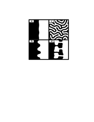
FIG. 4.: (a-d) Interface instability and labyrinth formation, Eq. (3), $\omega=2,b=4,\gamma=2.9$, domain size $100\times 100$ units, the snapshot are taken at times $t=1000,1600,2300,4640$.

The emergence of the labyrinthine patterns as a result of interface instability contradicts experiments [4, 5] where stable decorated interfaces are typically observed. Thus, the model Eq. (3) does not capture saturation of the interface instability and requires modification. We also checked that the coupling to the density field introduced in Ref. [13] also does not provide desired saturation.

Let us now discuss possible mechanisms of saturation of the transversal instability of the interface, which is not captured by Eq. (3). The reason for proliferation of the labyrinths is that local stabilization mechanisms cannot saturate the “negative surface tension instability” of the interface. Indeed, the behavior of small perturbation $\zeta$ of almost flat interface is described by the following linear equation: $\zeta_{t}=-\sigma\Delta\zeta$, where $\sigma$ is the surface tension. The linear growth must be counter-balanced by nonlinear terms. Due to translation invariance the local nonlinearity can be function of gradients of $\zeta$ only. In the lowest order the first term is $|\nabla\zeta|^{3}$, since the quadratic term does not saturate monotonic instability. Since for the modulation wavenumber $k\to 0$ one has $|\nabla\zeta|^{3}\sim k^{2}|\zeta|^{3}$ and $\Delta\zeta\sim k^{2}\zeta$, the linear instability always overcomes local nonlinearity at small wavenumbers. As a result small perturbations grow and saturation happens due to non-local interactions as in a labyrinthine pattern which is stabilized by non-local repulsion of the fronts (see [23]).

As we see, in our model the interface instability does not result in stable decorated interfaces. One of the possibility for the saturation of this instability could be local convection induced by the interface. Indeed, due to shear motion of grains at the interface (flat regions moves in anti-phase) local convective flow can be created. The scale of this flow can be large then the interface thickness. One of the possible manifestation of the convection beside grain transport is reduction of the effective ”viscosity” of flat layer, or increase in the sensitivity to external vibrations[24]. As we can see from Fig. 7 increase in vibration magnitude $\gamma$ suppresses the interface instability. As the instability develops, the length of the interface grows, which increases the convection and finally suppresses the instability. This feedback mechanism results in saturation of the interface instability and creates stable decorations.

Although the details of this coupling are not known yet, it can be implemented within the order-parameter approach in a phenomenological way. In Eq. 3 the forcing $\gamma\psi^{*}$ must be replaced by $(\gamma_{0}+w)\psi^{*}$, where $w$ includes the effect of local convective flow and $\gamma_{0}=const$. We take the simplest possible form of the coupling to the convective flow:

$$w=\frac{\epsilon}{S}\int dr^{\prime}\exp\left(-\frac{|r-r^{\prime}|^{2}}{r_{0}^{2}}\right)|\nabla\psi(r^{\prime})|^{2}$$ (29)

where $r_{0}$ characterizes the typical scale of the convective flow and $\epsilon$ is the amplitude of the coupling, and $S$ is the area of integration domain. Since $|\nabla\psi(r^{\prime})|$ is nonzero only at the interface, this integral is proportional to the total length of the interface. With the growth of the interface length the value of “effective forcing” $\gamma=\gamma_{0}+w$ grows as well, and eventually leaves the instability domain.

We performed numerical simulations with Eq. (3) modified in this fashion. The convolution integral (29) was calculated using the fast Fourier transform. The results are presented in Fig. 5. Remarkably, for certain range of parameters the instability indeed saturates due to nonlocal term Eq. (29), and we find interfaces with stable decorations, see Fig. 5,a.

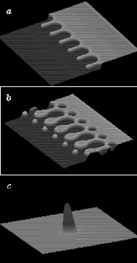
FIG. 5.: Computer simulations of modified Eq. (3). Surface plots show $Re\Psi$ for different stationary solutions: (a) the saturated interface, $\omega=1.2,\gamma=1.85,b=4$, $\epsilon=0.002$, $r_{0}=40$, $L=160$, (b) saturated interface with bound super-oscillons, $\omega=1.2,\gamma=1.75,b=4$, $\epsilon=0.002$, $r_{0}=40$, $L=160$. (c) single super-oscillon at $\omega=1.2,\gamma=2.2,b=4$, $\epsilon=0.002$, $r_{0}=40$, $L=100$ .

IV Localized Solutions

In addition to the interface solution which exists for $s>1$, Eq. (3) for even higher values of $s$ possesses a variety of other nontrivial two-dimensional solutions including localized ”super-oscillons”. The typical solution and its corresponding localized linear mode are shown in Fig. 6.

FIG. 6.: (a) Axi-symmetric localized solution (super-oscillon) obtained for $b=4,\omega=1$ and $\gamma=1.8$ for Eq. (3) at $b=4$, $A$-solid line, $B$- dashed line. (b) Localized eigenfunction corresponding to the maximum eigenvalue $\lambda=-0.0009$.

Although super-oscillon appears similar to the “conventional oscillon” discovered in Ref. [4], there is a significant difference. Asymptotic behavior of the super-oscillon is $\Psi\to A_{0}\neq 0$ for $r\to\infty$ whereas the regular oscillon has $\Psi\to 0$. As a result super-oscillons always have the same phase as their background. Oppositely-phased super-oscillons must be separated by the interface connecting two opposite phases of the period-doubled flat layer whereas oppositely-phased oscillons can form stable bound states (dipoles, [4]).

Super-oscillons exist in a relatively narrow domain of parameters of Eq. (3). Decrease of $\gamma$ leads to destabilization of the localized eigen-mode leading to subsequent nucleation of new ”super-oscillons” on the periphery of the unstable super-oscillon, with the increase of $\gamma$ super-oscillons disappear in a saddle-node bifurcation.

Interestingly, for certain values of $\gamma_{0}$ we also find an interesting structure consisting of a decorated interface and a chain of super-oscillons bound to the decorations, see Fig. 5,b. These objects can exist completely independently of the interface, Fig. 5 c, as one may expect for Eq. (3). Thus, we conclude that extended Eq. (3) qualitatively describes observed phenomenology.

V Phase diagram

The results of linear stability analysis can be summarized in the phase diagram shown in Fig. 7. Remarkably, the structure of the phase diagram Fig.7 is qualitatively similar to that of the experiments for high frequencies of vibration, see Fig. 10 and Refs. [2, 3, 4, 5, 9, 15]. Increasing vibration amplitude $\gamma$ leads to transition from a trivial state to stripes, hexagons, decorated interfaces, and finally, to stable interfaces. Transition from unstable to stable interfaces also occurs with decreasing $\omega$ (increasing vibration frequency $f$), in agreement with Ref.[15, 25]. In experiments, at yet higher $\Gamma$, quarter-harmonic patterns appear, however these patterns are not described by our model. Our analysis also predicts co-existence of stripes and hexagons in a very narrow parameter range (see Sec. II). Super-oscillons were found in a narrow domain close to line 7 of Fig. 7.

Note that square patterns which are emerge at lower frequencies, are not included in the phase diagram. They are obtained within the full model Eqs.(1),(2) with additional density field $\rho$, see [13].

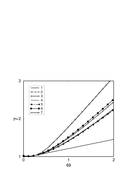
FIG. 7.: Phase diagram for Eq. (3) at $b=4$. Line 1, $\gamma^{2}=(\omega+b)^{2}/(1+b^{2})$; line 2, $s^{2}\equiv\gamma^{2}-\omega^{2}=1$; line 3, $s=s_{c}$; line 4, $s=s_{c}-\epsilon_{R}$; line 5, $s=s_{c}-\epsilon_{B}$; line 6, $s=s_{c}-\epsilon_{A}$; line 7, surface tension $\sigma=0$. Below line 1 there are no patterns, between lines 1 and 4 stripes are stable, between lines 5 and 6 hexagons are stable, above line 2, non-trivial flat states exist, and above line 3 they are stable. Interfaces are unstable below line 7. Hexagons and stripes coexist between lines $4$ and $5$

VI Swift-Hohenberg equation

Near the line $s=1$ (see Fig. 7) Eq. (3) can be simplified. In the vicinity of this line $A\sim(s-1)^{1/2}$ and $B\sim(s-1)^{3/2}\ll A$. In the leading order we can obtain from Eq. (5) $B=b\nabla^{2}A/2$, and Eq. (4) yields [26]:

$$\partial_{t}A=(s-1)A-A^{3}+(1-\omega b)\nabla^{2}A-\frac{b^{2}}{2}\ \nabla^{4}A.$$ (30)

Rescaling the variables $t\to(s-1)t,$ $A\to(s-1)^{-1/2}A,$ $x\to(2(s-1)/b^{2})^{1/4}$, we arrive to the Swift-Hohenberg equation (SHE)

$$\partial_{t}A=A-A^{3}-\delta\nabla^{2}A-\ \nabla^{4}A$$ (31)

where

$$\delta=\frac{\omega b-1}{b}\sqrt{\frac{2}{s-1}}.$$ (32)

The description by SHE is valid if $\delta\sim O(1)$ which implies additional condition for the validity of this approach $\omega b-1\ll 1$ at $s\to 1$.

Although this equation is simpler than Eq. (3), it captures many essential features of the original system dynamics, including existence and stability of stripes and hexagons in different parameter regions (see [27, 28]), existence of the interface solutions, interface instability, super-oscillons and emergence of labyrinthine patterns [29]. Indeed, simple analysis shows that the growth rate of the instability of the uniform state $A=1$ as a function of the perturbation wavenumber is determined by the formula $\lambda(k)=-2+\delta k^{2}-k^{4}$, so it becomes unstable at $\delta>\delta_{c}=2\sqrt{2}$ at critical wavenumber $k_{c}=\sqrt{2}$. As in the original model, near the threshold of this instability, subcritical hexagonal patterns are preferred. Interface stability can also be analyzed more simply as the linearized operator corresponding to the model (31) is self-adjoint. The threshold value of $\delta$ is obtained from the following solvability condition

$$\int_{-\infty}^{\infty}\left(\delta_{\mbox{th}}A_{0x}^{2}-2A_{0xx}^{2}\right)dx=0$$ (33)

which yields $\delta_{\mbox{th}}=1.011$. It yields the equation for the neutral curve of the interface instability in the Swift-Hohenberg limit in the form:

$$s=1+\frac{2(\omega b-1)^{2}}{\delta_{\mbox{th}}^{2}b^{2}}$$ (34)

Fig. 8, a-d shows the development of the interface instability within SHE with subsequent transition to labyrinthine patterns, similar to the dynamics of the full parametric equation (3). Again, to saturate the instability, an additional non-local mechanism is required.

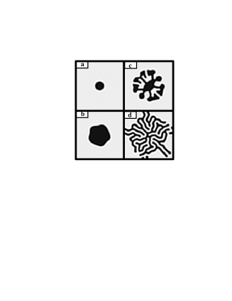
FIG. 8.: (a-d) labyrinth formation from a circular spot, SHE, $\delta=1.4$, domain size $100\times 100$ units, $t=200,1300,1700,1900$.

As it was shown recently, Swift-Hohenberg equation also possesses localized solutions (see [29, 30]). These localized states are analogous to the super-oscillons of Eq. (3).

VII Subharmonic forcing and interface motion

Let us focus on the effect of additional subharmonic driving on the motion of the interface. In the original model Eq. (3) the interface does not move due to symmetry between left and right halves of the interface. However, if the plate oscillates with two frequencies, $f$ and $f/2$, the symmetry between these two states connected by the interface, is broken, and interface moves. The velocity of interface motion depends on the relative phase of the sub-harmonic forcing with respect to the forcing at $f$. The effect of a small external subharmonic driving applied on the back-ground of primary harmonic driving with the frequency $f$ can be described by the following equation (cf. Eq. (3))

$$\partial_{t}\psi = \gamma\psi^{*}-(1-i\omega)\psi+(1+ib)\nabla^{2}\psi-|\psi|^{2}\psi+qe^{i\Phi}$$ (35)

where $q$ characterizes the amplitude of the sub-harmonic pumping, and $\Phi$ determines its relative phase.

For small $q$, we look for moving interface solution in the form $\psi=\psi_{0}(x-vt)+q\psi_{1}(x-vt)+...$ and $v=O(q)$, or, alternatively,

$${A\choose B}={A_{0}(x-vt)\choose B_{0}(x-vt)}+q{a(x-vt)\choose b(x-vt)}+O(q^{2})$$ (36)

Solvability condition (compare with Eq. (28)) fixes the interface velocity as a function of amplitude and the phase of external subharmonic driving

$$v=-q\frac{\cos\Phi\int{A^{+}dx}+\sin\Phi\int{B^{+}dx}}{\int{(A^{+}\partial_{x}A_{0}+B^{+}\partial_{x}B_{0})dx}}=q\alpha\sin(\Phi-\Phi_{0})$$ (37)

where $\alpha=const$ has the meaning of susceptibility of the interface for external forcing and $\Phi_{0}=const$ is some phase shift. The explicit answer is possible to obtain for $b=0$ when $A^{+}=\partial_{x}A_{0}$, and $\Phi=0,\pi$, which yields the interface velocity $v=\mp\frac{3}{2}qA_{0}^{-2}=\mp\frac{3}{2}q(s-1)^{-1}$. In general, $A,B$, $A^{+},B^{+}$, and hence $v$, can be found numerically. The interface velocity as function of $q,\Phi$ is shown in Fig. 9.

FIG. 9.: Interface velocity $v$ for $\omega=1,b=4,\gamma=2.5$ vs $q$ at $\Phi=0$. Inset: $v$ vs $\Phi$ at $q=0.01$. ($\bullet$) - numerical results, (—) - analytical expression (37).

Thus, from this analysis we conclude that additional subharmonic driving results in controlled motion of the interface. The velocity of the interface depends on the amplitude of the driving, and the direction is determined by the relative phase $\Phi$.

VIII Experimental results

We performed experiments with a thin layer of granular material subjected to periodic driving. Our experimental setup is similar to that of [5]. We used $0.15$mm diameter bronze or copper balls, and the layer thickness in our experiments was 10 particles. We performed experiments in a rectangular cell of $4\times 12$ cm². We varied the acceleration $\Gamma$ and the frequency $f$ of the primary driving signal as well as acceleration $\gamma$, frequency $f_{1}$ and the phase $\Phi$ of the secondary (additional) driving signal. The interface position and vertical accelerations were acquired using a high-speed video camera and accelerometers and further analyzed on a Pentium computer. To maintain and measure the proper acceleration at $f$ and $f/2$ we employ the lock-in technique with our signal originating from an accelerometer attached to the bottom of the cell. This allows for the simultaneous real-time feed back and control of the device. To reduce the interstitial gas effects[31] we reduced the pressure to 2 mTorr. Our visual data is acquired using a high speed digital camera (Kodak SR-1000c), in addition to high speed recording this also allows for a synchronization between the patterns and the image acquisition.

A Phase Diagram

The experimental phase diagram is shown in Fig. 10. It is similar to that of Ref. [3, 4], however the transition from hexagons to interfaces is elaborated in more detail. The dashed line indicates the stability line for interfaces with respect to periodic undulations. To determine this stability limit, we kept the value of acceleration $\Gamma$ fixed and increased the driving frequency $f$. For each value of the frequency we extracted the interface width by averaging up to 10 images of the interface. In order to find that amplitude of the periodic undulations $l$ we subtracted from the obtained value the thickness of the flat interface $l_{0}$. The resultant amplitude or undulations $l$ as function of driving frequency $f$ is shown in Fig. 11. As one sees from the Figure, the amplitude of undulations $l$ decreases gradually approaching the critical value of the frequency. However, a small hysteresis at the transition point cannot be excluded because of large error bars.

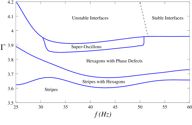
FIG. 10.: Phase diagram. Material is 150 $\mu m$ copper balls, layer thickness 10 particle diameters.

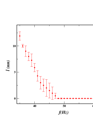
FIG. 11.: The amplitude of periodic undulations $l$ as a function of driving frequency $f$. The acceleration amplitude $\Gamma=4.1$

As it follows from the phase diagram, for small amplitude of the vertical acceleration $\Gamma<3.6$ stripes are the only stable pattern (note that we focus on high-frequency patterns when squares do not exist, compare [3]). At slightly higher $\Gamma=3.6..3.7$ stripes and hexagons coexist. For higher $\Gamma=3.7..4.0$ the hexagons becomes stable. Due to the sub-harmonic character of motion both up and down hexagons may co-exist separated by a line phase defect, Fig. 12,a. There exists a narrow band, from $\Gamma=3.85$ to $\Gamma=4.0$, where localized states, or super-oscillons, appear both within the bulk of the material and also pinned to the the front between the interface and the bulk Fig. 12,b. For even higher values of the acceleration $\Gamma>4.0$ the super-oscillons disappear (Fig. 12,c) leading to isolated interfaces with periodic decorations.

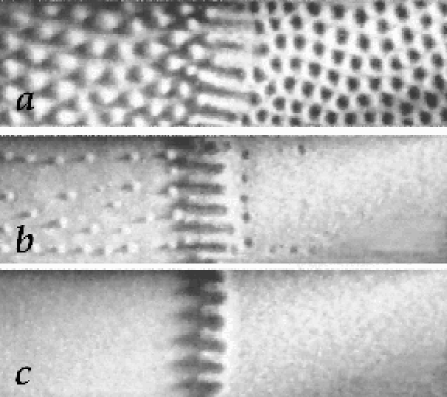
FIG. 12.: Representative high-acceleration patterns in the rectangular $4\times 12$ cm cell, driving frequency $f=40$ Hz: (a) $\Gamma=3.75$ shows the onset of the interface with up and down hexagons, (b) $\Gamma=3.94$ super-oscillons are present in the flat layer and are pinned to the front near the interface. (c) $\Gamma=4$, isolated decorated interface.

B Controlled Motion of Interface

In the absence of additional driving the interface drifts toward the middle of the cell (see Fig. 12). We attribute this effect to the feedback between the oscillating granular layer and the plate vibrations due to the finite ratio of the mass of the granular material to the mass of the vibrating plate. Even in the absence of subharmonic drive, the vibrating cell can acquire subharmonic motion from the periodic impacts of the granular layer on the bottom plate at half the driving frequency. If the interface is located in the middle of the cell, the masses of material on both sides of the interface are equal, and due to the anti-phase character of the layer motion on both sides, an additional subharmonic driving is not produced. The displacement of the interface $X$ from the center of the cell leads to a mass difference $\Delta m$ on opposite sides of the interface which in turn causes an additional subharmonic driving proportional to $\Delta m$. In a rectangular cell $\Delta m\propto X$. Our experiments show that the interface moves in such a way to decrease the subharmonic response, and the feedback provides an additional term $-X/\tau$ in the r.h.s. of Eq. (37), yielding

$$\frac{dX}{dt}=-X/\tau+q\alpha\sin(\Phi-\Phi_{0})$$ (38)

The relaxation time constant $\tau$ depends on the mass ratio (this also holds for the circular cell if $X$ is small compared to the cell radius). Thus, in the absence of an additional subharmonic drive ($q=0$), the interface will eventually divide the cell into two regions of equal area (see Fig. 12).

In order to verify the prediction of Eq. (38) we performed the following experiment. We positioned the interface off center by applying an additional subharmonic drive. Then we turned off the subharmonic drive and immediately measured the amplitude $\mu$ of the plate acceleration at the subharmonic frequency[32]. The results are presented in Fig. 13. The subharmonic acceleration of the cell decreases exponentially as the interface propagates to the center of the cell. The measured relaxation time $\tau$ of the subharmonic acceleration increases with the mass ratio of the granular layer and of the cell with all other parameters fixed. The mass of the granular layer was varied by using two different cell sizes: circular, diameter $15.3$ cm, and rectangular, $4\times 12$ cm, while keeping the thickness of the layer unchanged. For these cells we found that the relaxation time $\tau$ in the rectangular cell is about four times greater than for the circular cell (see Fig. 13). This is consistent with the ratio of the total masses of granular material (52 grams in rectangular cell and 198 grams in circular one). In a separate experiment the mass of the cell was changed by attaching an additional weight of 250 grams to the moving shaft, which weights 2300 grams. This led to an increase of the corresponding relaxation times of 15-25 %. The relaxation time $\tau$ increases rapidly with $\Gamma$ (see Fig. 13 inset).

FIG. 13.: Amplitude of the subharmonic acceleration $\mu$ of the cell averaged over 4 measurements vs time for the interface propagating to the center of the cell for $\Gamma=3.97$ and $f=40$ Hz. Circles/squares correspond to the circular/rectangular cells, open/closed symbols correspond to light/heavy cells, respectively. Heavy cells differ from light ones by an additional weight of 250 g attached to the moving shaft. Solid lines show exponential fit $\mu\sim\exp(t/\tau)+const$. Inset: $\tau$ vs $\Gamma$ for light rectangular cell.

When an additional subharmonic driving is applied, the interface is displaced from the middle of the cell. For small amplitude of the subharmonic driving $\gamma$, the stationary interface position is $X=q\alpha\tau\sin(\Phi-\Phi_{0})$, since the restoring force balances the external driving force. The equilibrium position $X$ as function of $\Phi$ is shown in Fig. 14a. The solid line depicts the sinusoidal fit predicted by the theory. Because of the finite mass ratio effect, the amplitude of the measured plate acceleration $\mu$ at frequency $f_{1}$ also shows periodic behavior with $\Phi$, (see Fig. 14b), enabling us to infer the interface displacement from the acceleration measurements. For even larger amplitude of subharmonic driving (more than 4-5 % of the primary driving) extended patterns (hexagons) re-emerge throughout the cell.

The velocity $V_{0}=q\alpha$ which the interface would have in an infinite system, can be found from the measurements of the relaxation time $\tau$ and maximum displacement $X_{m}$ at a given amplitude of subharmonic acceleration $\gamma$, $V_{0}=X_{m}/\tau$, see Eq.(38). We verified that in the rectangular cell the displacement $X$ depends linearly on $\gamma$ almost up to values at which the interface disappears at the short side wall of the cell (see Fig. 15, inset). Figure 15 shows the susceptibility $\alpha$ as a function of the amplitude of the primary acceleration $\Gamma$. The susceptibility decreases with $\Gamma$. The cusp-like features in the $\Gamma$-dependence of $\alpha$ (and $\tau$, see inset to Fig. 13), are presumably related to the commensurability between the lateral size of the cell and the wavelength of the interface decorations.

FIG. 14.: (a) Equilibrium position $X$ and (b) amplitude of measured subharmonic acceleration $\mu$ as functions of phase $\Phi$. Circular cell, $\Gamma=4.1$, $f=40$ Hz, $q=1.25\%$ of $\Gamma$.

FIG. 15.: Susceptibility $\alpha$ vs $\Gamma$ at $f=40$Hz, rectangular cell. Inset: Displacement $X$ as function of $q$ at $\Phi=260^{0}$.

We developed an alternative experimental technique which allowed us to measure simultaneously the relaxation time $\tau$ and the “asymptotic” velocity $V_{0}$. This was achieved by a small detuning $\Delta f$ of the additional frequency $f_{1}$ from the exact subharmonic frequency $f/2$, i.e. $\Delta f=f_{1}-f/2\ll f$. It is equivalent to the linear increase of phase shift $\Phi$ with the rate $2\pi\Delta f$. This linear growth of the phase results in a periodic motion of the interface with frequency $\Delta f$ and amplitude $X_{m}=V_{0}/\sqrt{\tau^{-2}+(2\pi\Delta f)^{2}}$ (see Eq (38)). The measurements of the “response functions” $X_{m}(\Delta f)$ are presented in Fig. 16. From the dependence of $X_{m}$ on $\Delta f$ we can extract parameters $V_{0},\alpha$ and $\tau$ by a fit to the theoretical function. The measurements are in a very good agreement with previous independent measurements of relaxation time $\tau$ and susceptibility $\alpha$. For comparison with the previous results, we indicate the values for $\tau$ and $\alpha$, obtained from the response function measurements of Figs. 13 and 15 (stars). The measurements agree within $5$ %.

FIG. 16.: Maximum displacement $X_{m}$ from center of rectangular cell as function of frequency difference $\Delta f=f_{1}-f/2$ for $f=40$ Hz, and for $\Gamma=3.97$ (circles) and $\Gamma=4.1$ (diamonds). Dashed lines are fit to $X_{m}=V_{0}/\sqrt{\tau^{-2}+(2\pi\Delta f)^{2}}$. The values of $\alpha$ and $\tau$ obtained from the fit are also indicated in Figs. 13 and 15 by arrows with stars.

IX conclusions

In this paper we studied the dynamics of thin vibrated granular layers in the framework of phenomenological model based on the Ginzburg-Landau type equation for the order parameter characterizing the amplitude of sub-harmonic sand vibrations. Although rigorous derivation of this model is not possible up to date, our approach gives a significant insight in the problem in hand and results in testable predictions. Our model is complementary to more elaborate fluid dynamics-like continuum descriptions or direct molecular dynamics simulations and allows us to carry out analytical calculations of various regimes and predict their stability. A challenging problem is to establish a quantitative relation between our order parameter model and other models and experiments.

We have shown in this paper that the generic parametric Ginzburg-Landau model Eq.(3) captures not only patterns of vibrated sand near the primary bifurcation, but also large acceleration patterns such as hexagons, interfaces, and super-oscillons. The structure of the phase diagram Fig.7 for high frequencies and amplitudes of vibrations is qualitatively similar to that of previous experiments Refs.[2, 3, 5, 15], as well as the experiments reported here. Increasing vibration amplitude leads to transition from a trivial state to stripes, hexagons, decorated interfaces, and finally, to stable interfaces. Interface decorations were found to be a result of the transversal instability of a flat interface which is analogous to the negative surface tension. We found that Eq. (3) is not sufficient to describe the saturation of interface instability. We propose a possible non-local mechanism of saturation of this instability which takes into account the dependence of the overall length of the interface and magnitude of parametric forcing, which may occur due to a large scale convective flow induced by the sand motion near the interface. We described analytically the motion of the interface under the symmetry-breaking influence of the small subharmonic driving.

In our experimental study we found that on a qualitative level the theoretical phase diagram is similar to the experimental one. The experiments also confirmed existence of super-oscillons and their bound states with the interface as it was predicted by the theory. Further experimental study is necessary to elucidate the specific mechanism for saturation of the interface instability.

Stimulated by the theoretical prediction, we also performed experimental studies of interface motion under additional subharmonic driving. The experiment confirmed that the direction and magnitude of the interface displacement depend sensitively on the amplitude and the relative phase of the subharmonic driving. Moreover, we found that period-doubling motion of the flat layers produces subharmonic driving because of the finite ratio of the mass of the granular layer and the cell. This in turn leads to the restoring force driving the interface towards the middle of the cell.

We thank L. Kadanoff, R. Behringer, H. Jaeger, H. Swinney and P. Umbanhowar for useful discussions. This research was supported by the US Department of Energy, grant # W-31-109-ENG-38, and by NSF, STCS #DMR91-20000. C.J. acknowledges support from joint ANL-UofC collaborative grant. L.T. thanks the Engineering Research Program of the Office of Basic Energy Sciences at the U.S. Department of Energy, grants #DE-FG03-96ER14592, DE-FG03-95ER14516 for support.

REFERENCES

- [1] H.M. Jaeger, S.R. Nagel, and R.P. Behringer, Physics Today 49, 32 (1996); Rev. Mod. Phys. 68, 1259 (1996).
- [2] F. Melo, P.B. Umbanhowar, and H.L. Swinney, Phys. Rev. Lett. 72, 172 (1994).
- [3] F. Melo, P.B. Umbanhowar, and H.L. Swinney, Phys. Rev. Lett.75, 3838 (1995).
- [4] P.B. Umbanhowar,F. Melo, and H.L. Swinney, Nature 382, 793-796 (1996); Physica A 249, 1 (1998).
- [5] I.S. Aranson, D. Blair, W. Kwok, G. Karapetrov, U. Welp, G. W. Crabtree, V.M. Vinokur, and L.S. Tsimring, Phys. Rev. Lett.82, 731 (1999).
- [6] T. H. Metcalf, J. B. Knight, H. M. Jaeger, Physica A 236, 202 (1997).
- [7] N. Mujica and F. Melo, Phys. Rev. Lett.80, 5121 (1998)
- [8] C. Bizon, M.D. Shattuck, J.B. Swift, W.D. McCormick, H.L. Swinney, Phys. Rev. Lett.80, 57 (1998)
- [9] J.R. De Bruyn, C. Bizon, M.D. Shattuck, D. Goldman, and H.L. Swinney, Phys. Rev. Lett.81, 1421 (1998)
- [10] S. Luding, E. Clement, J. Rajchenbach, and J. Duran, Europhys. Lett. 36, 247 (1996).
- [11] D. Rothman, Phys. Rev. E57 (1998); E. Cerda, F. Melo, and S. Rica, Phys. Rev. Lett.79, 4570 (1997); T. Shinbrot, Nature 389, 574 (1997); J. Eggers and H. Riecke, Phys. Rev. Lett.59, 4476 (1999); S. C. Venkataramani and E. Ott, Phys. Rev. Lett.80, 3495 (1998).
- [12] C. Crawford and H. Riecke, Physica D 129, 83 (1999)
- [13] L.S. Tsimring and I.S. Aranson, Phys. Rev. Lett.79, 213 (1997); I.S. Aranson and L.S. Tsimring, Physica A 249, 103 (1998).
- [14] I.S. Aranson, L.S. Tsimring, and V.M. Vinokur Phys. Rev. E59, 1327 (1999).
- [15] P.K. Das and D. Blair, Phys. Lett. A 242, 326 (1998).
- [16] Note that Eq.(3) also describes the evolution of the order parameter for the parametric instability in vertically oscillating fluids (see [17, 18]). However, unlike granular materials, fluid layer cannot leave the surface and therefore the non-trivial uniform states are prohibited.
- [17] W. Zhang and J. Vinals, Phys. Rev. Lett.74, 690 (1995).
- [18] S.V. Kiyashko, L.N. Korzinov, M.I. Rabinovich, and L.S. Tsimring, Phys. Rev. E54, 5037 (1996).
- [19] A. Mehta and J.M. Luck, Phys. Rev. Lett.65, 393 (1990).
- [20] M. Cross and P.C. Hohenberg, Rev. Mod. Phys. 65 851 (1993).
- [21] This analysis is similar to that of Ref. [27] where stability of hexagons was demonstrated for the SHE. In a certain limit Eq. (3) can be reduced to SHE (see below).
- [22] Numerical experiments were performed using quasi-spectral split-step method in a domain with mesh points and periodic boundary conditions.
- [23] D.M. Petrich and R.E. Goldstein, Phys. Rev. Lett.72, 1120 (1994); D.M. Petrich, D.J.Muraki, and R.E. Goldstein, Phys. Rev. E53, 3933 (1996).
- [24] The importance of large-scale flow was indirectly demonstrated also in Ref. [9].
- [25] P.B.Umbanhowar, Ph. Thesis, U.Texas, Austin, 1996.
- [26] SHE for oscillatory systems with strong resonance coupling was derived by P. Coullet and K. Emilson, Physica D 61, 119 (1992).
- [27] G. Dewel, S. Métens, M’F. Hilali, P. Borckmans and C.B. Price, Phys. Rev. Lett.74, 4647 (1995).
- [28] In Ref. [12] modified Swift-Hohenberg equations was used to describe squares and oscillons.
- [29] I. S. Aranson, B. A. Malomed, L. M. Pismen, and L. S. Tsimring, submitted to Phys. Rev. Lett.(1999).
- [30] K. Ouchi and H. Fujisaka, Phys. Rev. E54, 3895 (1996); K. Staliunas and V.J. Sánchez-Morcillo, Phys. Lett. A 241, 28 (1998).
- [31] H.K. Pak E. VanDoorn and R.P. Behringer Phys. Rev. Lett.74, 4643 (1995).
- [32] The measured acceleration may differ from the applied subharmonic (sinusoidal) driving since the granular material moves inside the cell. We measure independently by removing the granular material from the cell.