Spin correlation functions and Néel order in the 2D Heisenberg model: Effects of spatial anisotropy
C. Schindelin^a, D. Ihle^b, S.-L. Drechsler${}^{\rm\,c}$ and H. Fehske^{a a}Physikalisches Institut, Universität Bayreuth, D-95440 Bayreuth, Germany ^bInstitut für Theoretische Physik, Universität Leipzig, D-04109 Leipzig, Germany ^cInstitut für Festkörper- und Werkstofforschung Dresden e.V. D-01171 Dresden, Germany Abstract
      The ground-state properties of the square-lattice spin-1/2 Heisenberg antiferromagnet with spatially anisotropic couplings are investigated by Green’s-function projection approaches. The staggered magnetization and the two-spin correlators are calculated; the competition between magnetic long- and short-range order is discussed in comparison with experiments on $\rm Sr_{2}[Ca_{2}]CuO_{3}$. Keywords: spatial anisotropic Heisenberg model, magnetic short-range order, order-disorder transition
Motivated by experiments on quasi-1D quantum spin systems, such as $\rm Sr_{2}CuO_{3}$ and $\rm Ca_{2}CuO_{3}$ [1], many efforts were made to clarify the dimensional crossover in the square-lattice spin-1/2 antiferromagnetic (AFM) Heisenberg model [2, 3, 4]

$${\cal H}=\frac{J_{x}}{2}\Big{[}\sum_{\langle i,j\rangle_{x}}{\bf S}_{i}{\bf S}_{j}+R\sum_{\langle i,j\rangle_{y}}{\bf S}_{i}{\bf S}_{j}\Big{]}\,.$$ (1)

Here $R=J_{y}/J_{x}$ (throughout we set $J_{x}=1$), and $\langle i,j\rangle_{x,y}$ denote nearest neighbors along the $x$-, $y$-directions. In the ground state, the staggered magnetization reveals a transition from a long-range ordered (LRO) Néel state to a spin liquid with AFM short-range order (SRO) at the critical ratio $R_{c}$. Quantum Monte Carlo data provide strong evidence for $R_{c}=0$ [3], which also results from RPA theories [5, 1] and (multi-) chain mean-field approaches [3]. In previous work [4], based on a spin-rotation-invariant (SRI) Green’s function theory and Lanczos diagonalizations, we found a sharp crossover in the spatial dependence of the spin correlation functions at $R_{0}\simeq 0.2$.

In this paper we mainly focus on the SRO properties of the model (1) at $T=0$ studied by a generalized RPA theory compared with the SRI theory of Ref. [4]. Both approaches are based on the projection method for two-time retarded Green’s functions in calculating the dynamic spin susceptibility $\chi^{+-}({\bf q},\omega)=-\langle\langle S_{\bf q}^{+};S_{-{\bf q}}^{-}\rangle\rangle_{\omega}$.

\begin{picture}(70.0,74.0)\end{picture}

First, we extend the non-SRI theory of Ref. [6] to the case $R\neq 1$, hereafter referred to as theory I. Introducing two sublattices $(a,b)$ and taking the basis ${\bf A}=(S_{\bf q}^{a+},S_{\bf q}^{b+})^{T}$, where $S^{+}_{\bf q}=\frac{1}{\sqrt{2}}(S_{\bf q}^{a+}+S_{\bf q}^{b+})$, we get

$$\chi^{+-}({\bf q},\omega)=-\frac{M^{(1)}_{\bf q}}{\omega^{2}-\omega_{\bf q}^{2}}\,,$$ (2)

with $M_{{\bf q}}^{(1)}=-4C_{1,0}[1-\cos q_{x}+R\zeta(1-\cos q_{y})]$, $\zeta=C_{0,1}/C_{1,0}$, $C_{\bf r}=(C_{\bf r}^{+-}+2C_{\bf r}^{zz})/2\equiv C_{n,m}$, $C_{\bf r}^{+-}=\langle S_{\bf 0}^{+}S_{\bf r}^{-}\rangle=\frac{1}{N}\sum_{\bf q}\frac{M_{\bf q}^{(1)}}{2\omega_{\bf q}}\mbox{e}^{i{\bf q}{\bf r}}$, and ${\bf r}=n{\bf e_{x}}+m{\bf e_{y}}$. The magnon spectrum $\bar{\omega}_{\bf q}=\omega_{\bf q}/Z_{c}^{x}$ is

$$\bar{\omega}_{\bf q}^{2}=(1+R\zeta)^{2}-(\cos q_{x}+R\zeta\cos q_{y})^{2}\,,$$ (3)

where $Z_{c}^{x}=-2C_{1,0}/\langle S^{az}\rangle$. Using the identity $S_{i}^{z}=-\frac{1}{2}+S_{i}^{+}S_{i}^{-}$, the sublattice magnetization $m\equiv\langle S^{az}\rangle=-\langle S^{bz}\rangle$ is given by

$$m=\Big{[}\frac{2(1+R\zeta)}{N}\sum_{\bf q}\bar{\omega}_{\bf q}^{-1}\Big{]}^{-1}\,.$$ (4)

The theory contains one free parameter $\zeta$ which we fix by the requirement $C_{0,1}^{+-}/C_{1,0}^{+-}\stackrel{{\scriptstyle(!)}}{{=}}\zeta$. The spin-wave velocity renormalization factor $Z_{c}^{x}$ is calculated from $Z_{c}^{x}=(1+R)\Big{[}\frac{1}{N}\sum_{\bf q}\bar{\omega}_{\bf q}\Big{]}^{-1}$. In the RPA theory of Ref. [5], $m$ is given by Eqs. (4) and (3) with $\zeta\equiv 1$. For $R\ll 1$ we have $m=0.303[1-0.386\ln(R\zeta)]^{-1}$ [1].

In the SRI theory [4], hereafter referred to as theory II, the basis is chosen as ${{\bf A}=(S_{\bf q}^{+},i\dot{S}_{\bf q}^{+})^{T}}$ yielding $\chi^{+-}({\bf q},\omega)$ and $M_{\bf q}^{(1)}$ given by Eq. (2). The spectrum is calculated in the approximation $-\ddot{S}^{+}_{\bf q}=\omega_{\bf q}^{2}S^{+}_{\bf q}$, where $\omega_{\bf q}$ is expressed by correlation functions and vertex parameters. Again, one parameter is free and may be determined by adjusting either the ground-state energy per site $\varepsilon(R)$ [2] (case A), the uniform susceptibility (case B), or $m(R)$ [3] (case C) [ for details see Ref. [4]].

As seen in Fig. 1, the LRO in theory I is reduced compared with the RPA result [5] due to the ratio $\zeta$ expressing the SRO anisotropy. Considering, e.g., the ordered moment in $\rm Ca_{2}CuO_{3}$, where $R=0.023$ [1], in theory I we get $\zeta=0.157$ and $m=0.0956$ exceeding the experimental value [1] by a factor of about two, whereas the RPA and chain mean-field theory ($m=0.72\sqrt{R}$ at $R\ll 1$ [3]) yield $m=0.123$ and $m=0.109$, respectively. Comparing $\varepsilon(R)$ (inset) with the Ising expansion data of Ref. [2], theories I and II C (input $m(R)$ of Ref. [3], cf. Fig. 1) yield insufficient results at $R\stackrel{{\scriptstyle<}}{{\sim}}0.25$. On the other hand, in theory II B ($R_{c}\simeq 0.24$ [4]), $\varepsilon(R)$ nearly agrees with the exact data at $R\stackrel{{\scriptstyle<}}{{\sim}}0.25$. That is, in the Green’s-function theories describing LRO with $R_{c}=0$, the SRO at $R\stackrel{{\scriptstyle<}}{{\sim}}0.25$ is reproduced inadequately.

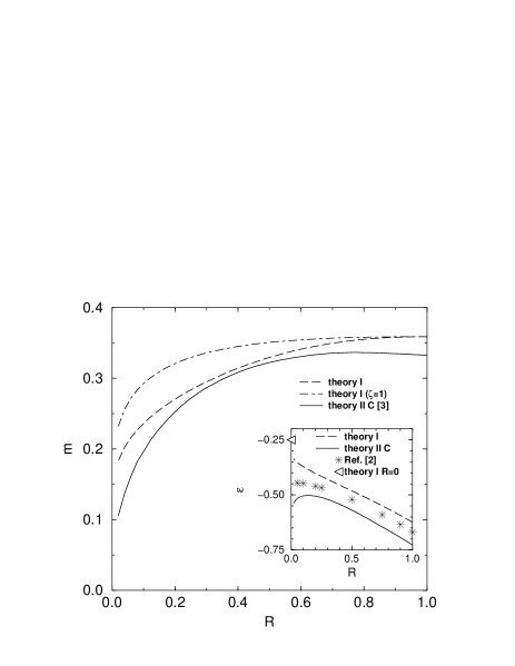
Figure 1: R-dependence of the magnetization $m$ and of the ground-state energy per site $\varepsilon$ (inset).

The same qualitative behavior can be seen from $C_{\bf r}$ depicted in Fig. 2. Compared with theory II A ($R_{c}\simeq 0.24$), where the correlators reasonably agree with the exact diagonalization data [4], theory I becomes unsatisfactory at $R\stackrel{{\scriptstyle<}}{{\sim}}0.25$. There we have $2|C_{1,0}^{zz}|\ll|C_{1,0}^{+-}|$ and, for $R<0.1$, $C_{1,0}^{zz}>0$ being incompatible with the AFM SRO. Equally, the correlators $C_{1,1}$ and $C_{2,0}$ (inset) in theory II C strongly deviate from those in theory II A at $R\stackrel{{\scriptstyle<}}{{\sim}}0.25$.

To conclude, our results call for an improved theory which may describe both the LRO and SRO equally well and explain the very small moments in $\rm Sr_{2}[Ca_{2}]CuO_{3}$.

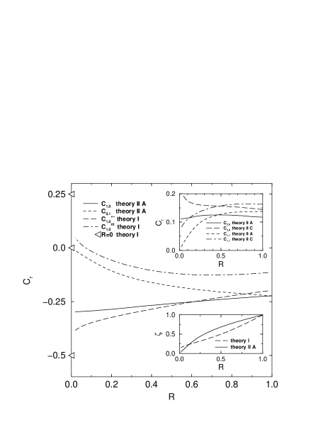
Figure 2: Nearest-neighbor and longer ranged (upper inset) spin correlation functions versus $R$. The lower inset demonstrates that there is no decoupling transition; i.e. $\zeta>0$ $\forall R$, contrary to the suggestion in [7].

References

[1]
H. Rosner, H. Eschrig, R. Hayn and S.-L. Drechsler,
J. Malek, Phys. Rev. B
56 (1997) 3402.
[2]
I. Affleck, M. P. Gelfand and R. R. P. Singh, J. Phys. A 27
(1994) 7313; 28 (E) (1995) 1787.
[3]
A. W. Sandvik, cond-mat//9904218.
[4]
D. Ihle, C. Schindelin, A. Weiße and H. Fehske, cond-mat/9904005.
[5]
N. Majlis, S. Selzer and G. C. Strinati, Phys. Rev. B 45 (1992) 7872;
ibid. 48, (1993) 957.
[6]
P. Krüger and P. Schuck, EuroPhys. Lett. 27 (1994) 395.
[7] A. Parola, S. Sorella and Q. F. Zhong,
Phys. Rev. Lett. 71 (1993) 4393.