Transition from quantum to classical Heisenberg trimers: Thermodynamics and time correlation functions

Abstract

We focus on the transition from quantum to classical behavior in thermodynamic functions and time correlation functions of a system consisting of three identical quantum spins $s$ that interact via isotropic Heisenberg exchange. The partition function and the zero-field magnetic susceptibility are readily shown to adopt their classical forms with increasing $s$. The behavior of the spin autocorrelation function (ACF) is more subtle. Unlike the classical Heisenberg trimer where the ACF approaches a unique non-zero limit for long times, for the quantum trimer the ACF is periodic in time. We present exact values of the time average over one period of the quantum trimer for $s\leq 7$ and for infinite temperature. These averages differ from the long-time limit, $(9/40)\ln 3+(7/30)$, of the corresponding classical trimer by terms of order $1/s^{2}$. However, upon applying the Levin $u$-sequence acceleration method to our quantum results we can reproduce the classical value to six significant figures.

PACS: 05.20.-y; 05.30.-d; 75.10.Hk; 75.10.Jm; 75.40.Cx; 75.40.Gb

Keywords: Quantum statistics; Canonical ensemble; Heisenberg model; Spin trimer; Levin u-sequence acceleration method

1 Introduction and summary

In recent years considerable attention has been devoted to the magnetic properties of synthesized organic complexes (“molecular magnets”) containing small numbers of paramagnetic ions [1, 2, 3, 4, 5]. With the ability to control the placement of magnetic moments of diverse species within stable molecular structures, it is now possible to test basic questions concerning their magnetic properties and to explore the design of novel systems that offer the prospect of useful applications [6, 7]. Intermolecular magnetic interactions are typically extremely weak compared to intramolecular interactions, so a bulk sample can be considered as independent individual molecular magnets.

The present study is motivated by the successful synthesis of two trimers, one [8] consisting of V⁴⁺ ions ($s=1/2$) and the second [9] consisting of Fe³⁺ ions ($s=5/2$). With the anticipation of the successful synthesis of yet other trimers, in this article we consider the thermodynamic functions and the time correlation functions for three identical quantum spins $s$ which interact via isotropic Heisenberg exchange in the absence of an external magnetic field. We are especially interested in comparing the behavior of these quantities for diverse $s$, and in particular in the transition to classical behavior which occurs for large $s$. This transition is readily analyzed for the thermodynamic functions. In particular, we show that the partition function and the zero-field magnetic susceptibility adopt the correct classical forms [10] with increasing $s$. Our analysis also provides results for the deviation from classical behavior depending on the size of $s$ and the temperature of the system.

Knowledge of the exact two-spin time correlation functions is of great importance since this enables one to predict the outcome of measurements such as the proton-spin lattice relaxation rate [11] by nuclear magnetic resonance (NMR) techniques and inelastic magnetic neutron scattering [12]. In an earlier publication [13] we examined in detail the properties of the thermal equilibrium autocorrelation function, to be denoted by $A_{s}(t,T)$, for a quantum Heisenberg dimer composed of two identical spins $s$ which interact with isotropic exchange. Some features of $A_{s}(t,T)$ that occur for a dimer are readily shown to occur for the trimer, too, and we will not deal with those issues. However, there are two features of $A_{s}(t,T)$ for the quantum trimer which deserve careful attention and these are considered in detail.

First, for the quantum Heisenberg trimers the quantity $A_{s}(t,T)$ is a periodic function of the time with a recurrence time $\tau$. For the corresponding classical Heisenberg trimer, whose ACF is denoted by $A_{c}(t,T)$, there exists a unique, non-zero long-time limit $A_{c}(\infty,T)$ [14]. To make a meaningful comparison between the asymptotic, long-time behavior of the classical Heisenberg trimer with a quantum trimer, we suggest comparing $A_{c}(\infty,T)$ with the time average of $A_{s}(t,T)$ over the corresponding recurrence time $\tau$, to be denoted by $\overline{A}_{s}(T)$; this value is equivalent to the coefficient of $\delta(\omega)$ in the expression for the Fourier time transform of $A_{s}(t,T)$. In particular we will explore the large $s$ behavior of $\overline{A}_{s}(T)$. Second, for the classical Heisenberg trimer, and for the special case of infinite temperature it has been shown that $A_{c}(\infty,\infty)=(9/40)\ln 3+7/30$ [14]. This curious exact value differs from the result, $1/N$, that follows from a phenomenological diffusive spin dynamics (DSD) [14] based on linear equations of motion for a ring of $N$, here $N=3$, interacting classical Heisenberg spins. By contrast, for both the quantum and classical dimers it has been found that $\overline{A}_{s}(\infty)=A_{c}(\infty,\infty)={\frac{1}{2}}$, independent of $s$ and in agreement with the DSD result. It is thus of interest to track the emergence of the exact classical result upon considering the sequence of quantum trimers for increasing $s$.

We have derived the exact values of $\overline{A}_{s}(\infty)$ for the quantum trimers for the choices $s=1/2,1,3/2,\dots,7$. It is necessary to consider the results for half-integer $s$ separately from those derived for integer $s$ since they exhibit different behaviour patterns. Each subsequence appears to converge very slowly to the above value of $A_{c}(\infty,\infty)$ for the classical trimer. For spins $s$ the deviation of $\overline{A}_{s}(\infty)$ from the classical result is of order $1/s^{2}$. However, when we apply the Levin $u$-sequence acceleration method [15, 16] to the subsequence for half-integer $s$ we arrive at an estimate for the large-$s$-limit which agrees to 6 significant figures with $A_{c}(\infty,\infty)$. For integer $s$ the Levin $u$-estimate agrees with $A_{c}(\infty,\infty)$ to 5 significant figures.

The layout of this paper is as follows. In Sec. 2 we calculate the partition function and the zero-field susceptibility of the quantum trimer for general $s$. We show that both quantities approach the corresponding results for the classical trimer. In Sec. 3 we derive a general formula for the time average $\overline{A}_{s}(\infty)$. Numerical evaluation of the formula becomes a very lengthy process with increasing $s$, however, we have been able to perform these calculations for $s\leq 7$. The Levin $u$-estimates for $\overline{A}_{s}(\infty)$ are also provided in Sec. 3.

2 Thermodynamic functions

The quantum trimer is specified by the Hamilton operator

$$\!\hbox{}\mathop{\vphantom{H}\smash{H}}\limits_{\sim}\!{}_{0} = \frac{J}{\hbar^{2}}\;\left(\!\hbox{}\mathop{\vphantom{{\!\vec{\,s}}}\smash{{\!\vec{\,s}}}}\limits_{\sim}\!{}_{1}\cdot\!\hbox{}\mathop{\vphantom{{\!\vec{\,s}}}\smash{{\!\vec{\,s}}}}\limits_{\sim}\!{}_{2}+\!\hbox{}\mathop{\vphantom{{\!\vec{\,s}}}\smash{{\!\vec{\,s}}}}\limits_{\sim}\!{}_{2}\cdot\!\hbox{}\mathop{\vphantom{{\!\vec{\,s}}}\smash{{\!\vec{\,s}}}}\limits_{\sim}\!{}_{3}+\!\hbox{}\mathop{\vphantom{{\!\vec{\,s}}}\smash{{\!\vec{\,s}}}}\limits_{\sim}\!{}_{3}\cdot\!\hbox{}\mathop{\vphantom{{\!\vec{\,s}}}\smash{{\!\vec{\,s}}}}\limits_{\sim}\!{}_{1}\right)$$

$$= \frac{J}{2\hbar^{2}}\;\left(\!\hbox{}\mathop{\vphantom{{\!\vec{\,S}}}\smash{{\!\vec{\,S}}}}\limits_{\sim}\!{}^{2}-\!\hbox{}\mathop{\vphantom{{\!\vec{\,s}}}\smash{{\!\vec{\,s}}}}\limits_{\sim}\!{}_{1}^{2}-\!\hbox{}\mathop{\vphantom{{\!\vec{\,s}}}\smash{{\!\vec{\,s}}}}\limits_{\sim}\!{}_{2}^{2}-\!\hbox{}\mathop{\vphantom{{\!\vec{\,s}}}\smash{{\!\vec{\,s}}}}\limits_{\sim}\!{}_{3}^{2}\right)\quad\ ;\quad\!\hbox{}\mathop{\vphantom{{\!\vec{\,S}}}\smash{{\!\vec{\,S}}}}\limits_{\sim}\hbox{}\!=\!\hbox{}\mathop{\vphantom{{\!\vec{\,s}}}\smash{{\!\vec{\,s}}}}\limits_{\sim}\!{}_{1}+\!\hbox{}\mathop{\vphantom{{\!\vec{\,s}}}\smash{{\!\vec{\,s}}}}\limits_{\sim}\!{}_{2}+\!\hbox{}\mathop{\vphantom{{\!\vec{\,s}}}\smash{{\!\vec{\,s}}}}\limits_{\sim}\!{}_{3}\ ,$$

where the spin operators satisfy the usual commutation relations and where $J$ has units of energy. $J>0$ describes antiferromagnetic and $J<0$ ferromagnetic coupling. Throughout this article it is assumed that the spin quantum numbers of the three sites are identical, $s_{1}=s_{2}=s_{3}=s$. The eigenstates $\,|\,{S,M,S_{23}}\,\rangle$ of the Hamilton operator can be chosen as simultaneous eigenstates of the total spin $\!\hbox{}\mathop{\vphantom{{\!\vec{\,S}}}\smash{{\!\vec{\,S}}}}\limits_{\sim}\!{}^{2}$, its $z$-component $\!\hbox{}\mathop{\vphantom{{S}}\smash{{S}}}\limits_{\sim}\!{}_{z}$, and of $\!\hbox{}\mathop{\vphantom{{\!\vec{\,S}}}\smash{{\!\vec{\,S}}}}\limits_{\sim}\!{}_{23}^{2}=(\!\hbox{}\mathop{\vphantom{{\!\vec{\,s}}}\smash{{\!\vec{\,s}}}}\limits_{\sim}\!{}_{2}+\!\hbox{}\mathop{\vphantom{{\!\vec{\,s}}}\smash{{\!\vec{\,s}}}}\limits_{\sim}\!{}_{3})^{2}$. The quantum numbers $S,M,S_{23}$ characterize the eigenstates completely. The eigenvalues $E_{S}$ of the Hamilton operator

$$E_{S} = \frac{J}{2}\;\left(S(S+1)-3\,s(s+1)\right)$$ (2)

do not depend on $S_{23}$ or $M$. Thus the partition function in the canonical ensemble reads

$$Z = \mbox{tr}\left\{e^{-\beta\!\hbox{}\mathop{\vphantom{H}\smash{H}}\limits_{\sim}\!{}_{0}}\right\}=\sum_{S,M,S_{23}}\langle\,{S,M,S_{23}}\,|\,e^{-\beta\!\hbox{}\mathop{\vphantom{H}\smash{H}}\limits_{\sim}\!{}_{0}}\,|\,{S,M,S_{23}}\,\rangle\ .$$ (3)

The respective classical Hamilton function $H_{c}$ is defined as [13]

$$H_{c}=J_{c}\;\left({\!\vec{\,e}}_{1}\cdot{\!\vec{\,e}}_{2}+{\!\vec{\,e}}_{2}\cdot{\!\vec{\,e}}_{3}+{\!\vec{\,e}}_{3}\cdot{\!\vec{\,e}}_{1}\right)\quad,\quad J_{c}=J\,s(s+1)\ ,$$ (4)

where ${\!\vec{\,e}}_{1}$, ${\!\vec{\,e}}_{2}$ and ${\!\vec{\,e}}_{3}$ are unit vectors (c-numbers). Then the classical partition function turns out to be [10]

$$Z_{c}=\int\,\mbox{d}E\,D_{c}(E)\exp(-\beta E)\ ,$$ (5)

with the classical density of states

$$D_{c}(E)=\left\{\begin{array}[]{l@{\quad:\quad}l}\vspace{2mm}\frac{1}{2J_{c}}\sqrt{\frac{2E}{J_{c}}+3}&-\frac{3}{2}\;J_{c}\leq E\leq-J_{c}\\ \vspace{2mm}\frac{1}{4J_{c}}(3-\sqrt{\frac{2E}{J_{c}}+3})&-J_{c}<E\leq 3J_{c}\\ 0&\mbox{else}\end{array}\right.\ ,$$ (6)

which is normalized to unity. In order to compare quantum and classical density of states, the energy spectra of the quantum trimers for different $s$ have to be mapped onto the same energy interval; we take $[-3J_{c}/2,3J_{c}]$, i.e. all energies are divided by $s(s+1)$.

Figure 1: Normalized density of states for quantum Heisenberg trimers (dashed lines) and their classical counterpart (solid line).

Figure 1 demonstrates how the quantum density of states approaches the classical limit with increasing spin $s$. Considering the eigenvalues (2) of the Hamilton operator (2) and their multiplicities, which originate from the degeneracy in the magnetic quantum number $M$ and from different possibilities to couple to a certain total spin $S$, one can show analytically that the quantum density of states converges against the classical one for infinite $s$ [17].

But the coincidence of the classical and the quantum density of states for high spin does not mean that other observables coincide, too. An interesting example is given by the zero field susceptibility. The susceptibility is defined as the derivative of the magnetisation

$${\mathcal{M}} = \frac{1}{Z}\,\mbox{tr}\left\{-g\mu_{B}\!\hbox{}\mathop{\vphantom{S}\smash{S}}\limits_{\sim}\!{}_{z}\mbox{e}^{-\beta\!\hbox{}\mathop{\vphantom{H}\smash{H}}\limits_{\sim}\hbox{}\!}\right\}\quad,\quad\!\hbox{}\mathop{\vphantom{H}\smash{H}}\limits_{\sim}\hbox{}\!=\!\hbox{}\mathop{\vphantom{H}\smash{H}}\limits_{\sim}\!{}_{0}+g\mu_{B}B\!\hbox{}\mathop{\vphantom{{S}}\smash{{S}}}\limits_{\sim}\!{}_{z}$$ (7)

with respect to the magnetic field $B$

$$\chi_{0} = \left(\frac{\partial\,{{\mathcal{M}}}}{\partial\,{B}}\;\right)_{B=0}=g^{2}\mu_{B}^{2}\beta\left(\frac{1}{Z}\,\mbox{tr}\left\{\left(\!\hbox{}\mathop{\vphantom{S}\smash{S}}\limits_{\sim}\!{}_{z}\right)^{2}\mbox{e}^{-\beta\!\hbox{}\mathop{\vphantom{H}\smash{H}}\limits_{\sim}\hbox{}\!}\right\}\right)_{B=0}\ .$$ (8)

For ferromagnetic coupling, Fig. 2 r.h.s., the graphs for different $s$ nearly coincide with each other and with the classical result. However, for antiferromagnetic coupling the zero field susceptibility behaves differently for integer and half-integer spin quantum numbers as shown on the l.h.s. of Fig. 2. The reason is that for integer spin the ground state, which is non-degenerate, has $S=0$ and thus the zero field susceptibility approaches zero for small temperatures $T$, whereas for half-integer spins the ground state, which is fourfold degenerate, has $S=1/2$ which causes the susceptibility to go to infinity for small $T$. However, if we consider a fixed nonzero value of $T$, the susceptibilities tend to the classical result with increasing $s$. The classical result is “indifferent” at $T=0$, it approaches $1$.

   

Figure 2: Zero-field susceptibility for $N=3$ and choices $s=1/2,1,\dots,9$. The solid lines show the result for half integer spins, the dashed lines for integer spin quantum numbers. The classical result is given by the thick dotted line. L.h.s.: antiferromagnetic coupling, r.h.s.: ferromagnetic coupling.

3 Autocorrelation function

Another important observable is the two-spin time correlation function because it serves as a major ingredient for several quantities such as the spin lattice relaxation rate and the neutron scattering cross section.

Considering that the Hamilton operator (2) is isotropic, one obtains for the autocorrelation function

$$A_{s}(t,T) = \frac{\mbox{Re}\left(\sum_{S,M,S_{23}}\langle\,{S,M,S_{23}}\,|\,\!\hbox{}\mathop{\vphantom{{s}}\smash{{s}}}\limits_{\sim}\!{}_{1z}(t)\cdot\!\hbox{}\mathop{\vphantom{{s}}\smash{{s}}}\limits_{\sim}\!{}_{1z}(0)\,e^{-\beta\!\hbox{}\mathop{\vphantom{H}\smash{H}}\limits_{\sim}\!{}_{0}}\,|\,{S,M,S_{23}}\,\rangle\right)}{\sum_{S,M,S_{23}}\langle\,{S,M,S_{23}}\,|\,\!\hbox{}\mathop{\vphantom{{s}}\smash{{s}}}\limits_{\sim}\!{}_{1z}(0)\cdot\!\hbox{}\mathop{\vphantom{{s}}\smash{{s}}}\limits_{\sim}\!{}_{1z}(0)\,e^{-\beta\!\hbox{}\mathop{\vphantom{H}\smash{H}}\limits_{\sim}\!{}_{0}}\,|\,{S,M,S_{23}}\,\rangle}\ .$$ (9)

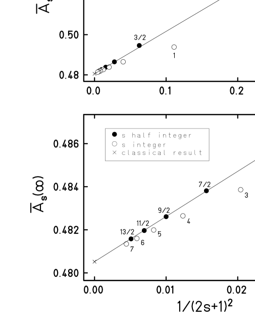
Figure 3: Results for $\overline{A}_{s}(\infty)$ (open and full circles) and $A_{c}(\infty,\infty)$ (cross). The line, which connects the results for $s=11/2$ and $s=13/2$, is drawn to guide the eye.

Since $\langle\,{S,M,S_{23}}\,|\,\!\hbox{}\mathop{\vphantom{{s}}\smash{{s}}}\limits_{\sim}\!{}_{1z}\,|\,{S^{\prime},M^{\prime},S_{23}^{\prime}}\,\rangle$ is zero if $|S-S^{\prime}|>1$, the contributing frequencies are $\omega=J(S+1)/\hbar$. They are all multiples of a basic frequency, which is $\omega_{r}=J/\hbar$ for integer spin quantum numbers and $\omega_{r}=J/(2\hbar)$ for half integer spin quantum numbers. Thus the autocorrelation function is periodic with a recurrence time $2\pi/\omega_{r}$.

We have evaluated the expression $\overline{A}_{s}(\infty)$

$$\overline{A}_{s}(\infty) = \lim_{T\rightarrow\infty}\int_{0}^{\frac{2\pi}{\omega_{r}}}\mbox{d}t\;A_{s}(t,T)$$ (10)

for half-integer values $1/2\leq s\leq 13/2$ and for integer values $1\leq s\leq 7$, and these are listed in table 1. It appears to be impractical to extend these results to larger spin values since the amount of computer time required grows at an astonishing rate with increasing $s$. Fortunately additional calculations are unwarranted. In Fig. 3 we display our results versus the independent variable $1/(2s+1)^{2}$ along with the solid line which has been chosen to pass through the quantum results for s=11/2 and s=13/2. The good agreement between the results for the larger half-integer values of $s$ and the solid line is consistent with the conclusion that the deviation between the quantum results and the classical trimer decreases monotonically to zero but very slowly, the deviation being of order $1/(2s+1)^{2}$. In fact, if we approximate $\overline{A}_{s}(\infty)$ by the form

$$\overline{A}_{s}(\infty)=A+\frac{B}{(2s+1)^{2}}\ ,$$ (11)

we may use our results for $s=11/2$ and $13/2$ to determine the unknown parameters $A$ and $B$. In particular the result $A=0.480511$ provides an estimate for $lim_{s\rightarrow\infty}\overline{A}_{s}(\infty)$. This result is rather close to the exact classical result [14]

$$A_{c}(\infty,\infty)=(9/40)\ln 3+7/30=0.4805210983\ .$$ (12)

Adopting Eq. (11) for the case of integer values of $s$ and using our results for $s=6$ and $s=7$ we find that $A=0.480575$.

We may obtain an improved estimate for $lim_{s\rightarrow\infty}\overline{A}_{s}(\infty)$ by exploiting the Levin $u$-sequence acceleration method [15, 16] which is tailor-made for such slowly convergent, monotonic sequences as the ones we face. If the sequence elements are labelled $U_{1},U_{2},U_{3},\dots$ (to be identified with $\overline{A}_{1/2}(\infty),\overline{A}_{3/2}(\infty),\dots$) and if we define the quantities $u_{1}=U_{1},u_{2}=U_{2}-U_{1},u_{3}=U_{3}-U_{2},\dots$ then the Levin $u$-estimate for $lim_{n\rightarrow\infty}U_{n}$ based on employing the first $M$ values of $U_{n}$ is given by

$$U[M]=\frac{\sum_{k=1}^{M}(-1)^{k-1}\binom{M}{k}k^{M-2}\frac{U_{k}}{u_{k}}}{\sum_{k=1}^{M}(-1)^{k-1}\binom{M}{k}k^{M-2}\frac{1}{u_{k}}}\ .$$ (13)

We find that $U[7]=0.48052085\dots$. For the corresponding sequence of integer values of $s$ we find that $U[7]=0.4805179\dots$.

It is interesting to note that for half-integer values of $s$ the Levin $u$-estimates are closer to the exact classical result than those for integer $s$.

$s$	$\overline{A}_{s}(\infty)$	$s$	$\overline{A}_{s}(\infty)$
1/2	$\frac{5}{9}=0.55555556$	1	$\frac{40}{81}=0.49382716$
3/2	$\frac{779}{1575}=0.49460317$	2	$\frac{5473}{11250}=0.48648889$
5/2	$\frac{986093}{2027025}=0.48647303$	3	$\frac{59747}{123480}=0.48385973$
7/2	$\frac{21117673}{43648605}=0.48381095$	4	$\frac{464441}{962280}=0.48264642$
9/2	$\frac{302812778207}{627448696875}=0.48260962$	5	$\frac{26536}{55055}=0.48199074$
11/2	$\frac{2796327017071}{5801928464475}=0.4819651$	6	$\frac{33240299}{69020952}=0.48159723$
13/2	$\frac{19699872589701257}{40906818968140125}=0.48157919$	7	$\frac{11459968711}{23808330000}=0.48134282$

Table 1: Time average, $\overline{A}_{s}(\infty)$, of the quantum autocorrelation function in the high-temperature limit for $s=1/2,1,\dots,7$.

References

- [1] A. Bencini, D. Gatteschi, Electron parametric resonance of exchange coupled systems, Springer, Berlin, Heidelberg (1990)
- [2] D. Gatteschi, A. Caneschi, L. Pardi, R. Sessoli, Large clusters of metal ions: The transition from molecular to bulk magnets, Science 265 (1994) 1054
- [3] D. Gatteschi, Molecular magnetism: A basis for new materials, Adv. Mater. 6 (1994) 635
- [4] J. Friedman, M.P. Sarachik, J. Tejada, R. Ziolo, Macroscopic measurement of resonant magnetization tunneling in high-spin molecules, Phys. Rev. Lett. 76 (1996) 3830
- [5] B. Pilawa, R. Desquiotz, M.T. Kelemen, M. Weickenmeier; A. Geisselman, Magnetic properties of new Fe6 (triethanolaminate(3-))6 spin clusters, J. Magn. Magn. Mater. 177 (1997) 748
- [6] A. Hernando (ed.), Nanomagnetism, NATO Applied Sciences, vol. 247, Kluwer Academic Publishing (1993)
- [7] R.J. Bushby, J.P. Paillaud, in Introduction to molecular electronics, edited by M.C. Petty, M.R. Bryce, D. Bloor, Oxford University Press, New York (1995) 72–91
- [8] A. Müller, J. Meyer, H. Bögge, A. Stammler, A. Bota, Trinuclear Fragments as Nucleation Centres: New Polyoxoalkoyvanadates by (induced ) Self-Assembly, Chem. Eur. J. 4 (1998) 1388
- [9] A. Caneschi, A. Cornia, A.C. Fabretti, D. Gatteschi, W. Malavasi, Polyiron(III)-Alkoxo Clusters: A novel Trinuclear Complex and Its Relevance to the Extended Lattices of Iron Oxides and Hydroxides, Inorg. Chem. 34 (1995) 4660
- [10] O. Ciftja, M. Luban, M. Auslender, J.H. Luscombe, Equations of state and spin correlation functions of ultra-small classical Heisenberg magnets, accepted for Phys. Rev. B (1999)
- [11] T. Moriya, Nuclear magnetic relaxation in antiferromagnets, Prog. Theor. Phys. 16 (1956) 23
- [12] E. Balcar, S.W. Lovesey, Theory of magnetic neutron and photon scattering, Clarendon, Oxford (1989)
- [13] D. Mentrup, J. Schnack, M. Luban, Spin dynamics of quantum and classical Heisenberg dimers, Physica A 272 (1999) 153
- [14] M. Luban, T. Bandos, and O. Ciftja, Exact time correlation functions for small classical Heisenberg magnets, in preparation
- [15] D. Levin, Development of non-linear transformations for improving convergence of sequences, Intern. J. Computer Math. B 2 (1973) 371
- [16] M. Luban Acceleration of convergence of the 1/d expansion for the critical temperature of the spherical model, Prog. Theor. Phys. 58 (1977) 1177
- [17] D. Mentrup, Untersuchungen zu kleinen Heisenberg-Spin-Systemen diploma thesis, University of Osnabrück (1999), available on request