Cluster-Growth in Freely Cooling Granular Media

Abstract

When dissipative particles are left alone, their fluctuation energy decays due to collisional interactions, clusters build up and grow with time until the system size is reached. When the effective dissipation is strong enough, this may lead to the “inelastic collapse”, i.e. the divergence of the collision frequency of some particles. The cluster growth is an interesting physical phenomenon, whereas the inelastic collapse is an intrinsic effect of the inelastic hard sphere (IHS) model used to study the cluster growth – involving only a negligible number of particles in the system. Here, we extend the IHS model by introducing an elastic contact energy and the related contact duration $t_{c}$. This avoids the inelastic collapse and allows to examine the long-time behavior of the system. For a quantitative description of the cluster growth, we propose a burning–like algorithm in continuous space, that readily identifies all particles that belong to the same cluster. The criterion for this is here chosen to be only the particle distance.

With this method we identify three regimes of behavior. First, for short times a homogeneous cooling state (HCS) exists, where a mean-field theory works nicely, and the clusters are tiny and grow very slowly. Second, at a certain time which depends on the system’s properties, cluster growth starts and the clusters increase in size and mass until, in the third regime, the system size is reached and most of the particles are collected in one huge cluster.

Lead paragraph

Granular media consist of discrete particles and their interaction is governed by two major concepts: excluded volume and dissipation. Adhesive and frictional forces are neglected in this study for the sake of simplicity. Since the particles are solid, each particle occupies a certain amount of space, and no other particle may enter this volume. If another particle approaches, the pair eventually collides. During collisions, energy is lost from those degrees of freedom (linear motion) which are important for the behavior of the material. Heat or sound is radiated and plastic deformation takes place so that energy is irreversibly gone.

Already such a simple, classical system shows an enormous number of interesting phenomena like, e.g., shock-waves, size-segregation, surface-waves, or the clustering in freely cooling systems. The latter will be examined more closely here. Since granular particles dissipate energy, the multi-particle system is usually not in equilibrium. This leads to various complex, non-linear phenomena, as mentioned above. In this study, we use a rather simple simulation method for inelastic, hard spheres, and examine the time dependent size of “clusters”, i.e. collections of particles whose nearest-neighbor separation is much smaller than the particle size. We propose a burning–type algorithm to identify those particles which belong to one cluster. Our new approach is a simple alternative to the analysis involving fourier spectra and structure factors or mode coupling-theory.

1 Introduction

An essential difference between a classical gas and a granular medium is the dissipation of energy. In a classical, conservative system in equilibrium, energy is conserved. In a dissipative system, the energy loss is quantified by the restitution coefficient $r$ that describes the ratio of the relative velocities of a pair of particles after and before the collision so that $r=1$ corresponds to the perfectly elastic situation. In dissipative granular systems with $r<1$ and only weak energy input, the phenomenology can be very rich [1, 2]. In this study we focus on the clustering phenomenon. Starting with a homogeneous density, one observes, after a short time, the evolution of patterns: Clusters of particles form and grow with time [3, 4]. This leads to the coexistence of almost empty regions and areas where the particles are densely packed. This is a general scenario in dissipative systems, rather independent of the details of the interaction.

The cluster formation may be understood in a qualitative manner: The homogeneous state contains density and velocity fluctuations. Convergent velocity fluctuations can lead to increasing densities in certain regions. As the collision rate increases in these regions, so does the energy dissipation rate. If the energy dissipation rate is great enough, the pressure cannot reverse the convergent flow and, if this process is not terminated by sufficiently strong perturbations, it is self-stabilizing, causes clusters and may eventually lead to the “inelastic collapse”. Note that inelastic collapse is not another expression for clustering, rather it describes the divergence of the collision frequency in the system, possibly involving a few particles only.

The size of the clusters, and thus one of the typical lengths of the system, grows until the system size is reached [3, 4, 5]. The beginning of cluster growth can also be explained by means of a hydrodynamic stability analysis [4, 6]. Clusters build up only if the effective density or dissipation is large enough. In the other case, the fluctuations of the kinetic energy can act as perturbations and destroy evolving clusters so that the system stays homogeneous. In intermediate situations shear modes are observed, for example see [4].

The clustering instability and the inelastic collapse were carefully examined in 1D [7, 8, 9, 10, 11, 12, 13], and in 2D [14, 3, 15, 16, 4, 17, 18, 19, 5]; systematic three dimensional studies were not performed to our knowledge. Dissipation reduces the fluctuation velocities and thus reduces the free volume. A decreasing free volume can lead to disorder–order transitions [20] and the inelastic collapse [4]. The inelastic collapse is due to the perfectly rigid interaction potential of the particles in the frequently used inelastic hard-sphere (IHS) model. Those potentials allow instantaneous contacts and thus a diverging number of collisions within small time-intervals.

In theoretical approaches, simplifying assumptions are made to keep the system tractable, these are, e.g., constant density, weak dissipation, and vanishing gradients of the field variables [21, 22, 23, 24]. A phenomenon like cluster growth cannot be described easily in the case of strong dissipation, where it is usually observed. Even if the global density is small and initially homogeneous, the density can get large locally and large gradients at the boundary between the clusters and the “vacuum” exist. For low densities and weak dissipation, the predictions of kinetic theory and stability analysis are true [4] and in the case of a homogeneous density, a perfect agreement between numerical simulations and kinetic theory was obtained for inelastic, rough, spherical particles in 2D and 3D also for high densities [25].

In order to model clustering, the inelastic hard sphere (IHS) model is frequently used, since the event driven nature of the modelling algorithm allows simulations over many orders of magnitude in time [25, 5]. The only drawback is the occurence of the inelastic collapse due to the rigid nature of contacts. In the framework of the IHS, the inelastic collapse is related to a divergence of the collision frequency and a vanishing particle separation and relative velocity. Different possibilities to avoid the unphysical inelastic collapse were proposed, and are reviewed in Ref. [5]. One of them introduces a virtual time of contact (TC), as also used in the following. The so-called TC model was examined in detail and seems to influence only a small fraction of the particles in the system [5]. The idea is to introduce an elastic energy which cannot be dissipated. When two particles are in contact, energy is stored in the deformed contact volume. This contact energy is not dissipated, but eventually converted into kinetic energy when the particles separate. In the TC model, particles that collide too frequently, i.e. more than once in a time-interval $t_{c}$, are assumed to be in contact, and their kinetic energy is not dissipated by further collisions. The time $t_{c}$ can be identified as the contact duration. The contact energy cannot be dissipated so that the collision frequency cannot diverge further, which implies that also the relative velocity and the separation cannot decrease further.

Using the TC model, vibrated [26, 27] and freely cooling [5] systems were examined in detail. For sufficiently weak dissipation, the homogeneous cooling state (HCS) is observed. In the HCS only a negligible number of particles collide twice within a short time $t_{c}$. If dissipation becomes stronger, clusters build up and the collision frequency inside the clusters increases. In this situation, the TC model is active, i.e. dissipation is switched off during a considerable number of collisions, and thus limits the steady increase of the collision frequency in the centers of the clusters. However, even when the collision frequency is strongly influenced by the TC model, the global cooling, i.e. the energy of the system, is almost unaffected. Furthermore, one observes that the TC model is able to avoid the inelastic collapse in the case of very strong dissipation, i.e. very small restitution coefficients $r$, and also in the case of large systems, where clusters can grow correspondingly [5].

In the following, we use the TC model extension of the IHS to investigate the freely cooling granular system. The homogeneous cooling state is discussed in section 2, and the influence of the parameters $r$ and $t_{c}$ is examined using small systems in section 3. Cluster growth in large systems is presented in section 4, and its quantitative analysis with a “burning”-type algorithm is introduced in section 5.

2 The homogeneous cooling state

In order to examine a system with homogeneous density, it is convenient to use periodic boundary conditions [28]. In a periodic, freely cooling system, given an isotropic initial condition, each point is a-priori identical to every other point, besides fluctuations in the initial configuration. In such a system without walls and without externally applied gradients in, say, temperature, the system has the chance to stay homogeneous; the presence of walls or other external forces can cause inhomogeneities which are thus due to the boundaries, but not intrinsic to the material. If the system is prepared with a homogeneous density and, as usual, relaxed for a certain time without dissipation, $r=1$, so that a Maxwell-Boltzmann velocity distribution is achieved, one has a starting configuration that allows examination of both the homogeneous cooling state (HCS) and the growth of clusters. The HCS occurs as long as dissipation is small, and fluctuations remain strong enough to disrupt the formation of clusters.

The dimensionless kinetic energy $K=E(t)/E(0)$ of a freely cooling system (where $E(t)$ is the kinetic translational energy), is well predicted by the analytical solution for the HCS of smooth particles (see Ref. [29] and references therein):

$$K=\left({1+\frac{1-r^{2}}{4}~{}\tau}\right)^{-2}~{}.$$ (1)

In Eq. (1) $\tau=t_{E}^{-1}(0)\,t$ is the time rescaled with the Enskog collision rate

$$t_{E}^{-1}(t)=2d\frac{N}{V}\sqrt{\pi\frac{E(t)}{M}}\,g(2a)$$ (2)

at time $t=0$, with the particle diameter $d$, the particle number $N$, the system volume $V$, the total particle mass $M=Nm$, and the particle-particle correlation function at contact $g(2a)$ [5]. The decay of energy in the rescaled time frame depends only on $r$, and all dependencies on quantities like system size and density are hidden in $\tau$.

3 Effect of $r$ and $t_{c}$

In the following, systems of length $L=l/d$ with $N$ particles of diameter $d$ are examined with event driven (ED) simulations [25, 5] in two dimensions (2D). The volume fraction is defined as $\varrho=N\pi(d/2l)^{2}=(\pi/4)N/V$. Initially the particles are arranged on a square lattice with random velocities drawn from an interval with constant probability for each coordinate. The mean total velocity, i.e. the random momentum due to the fluctuations, is disregarded in order to have a system with its center of mass at rest. The system is evolved for some time, until the arbitrary initial condition is forgotten, i.e. the density is homogeneous, and the velocity distribution is a Gaussian in each coordinate.

From those initial configurations, the simulation is started with $r<1$ at time $t=0$. In 2D the dimensionless kinetic energy $K=E(t)/E(0)=K_{x}+K_{z}$ has two contributions, one from each direction $x$ and $z$. If the system is isotropic $K_{x}\approx K_{z}$, and on the other hand, if shear modes or clusters are present, one of the components usually dominates. The first set of simulations concerns a small system with $N=784$, $L=50$, $t_{c}=10^{-5}$ s, and $\varrho\approx 0.25$. Simulations are performed for different $r=0.99$, 0.97, 0.95, 0.9, 0.8, 0.6, and 0.2 until every particle carried out $C/N=1000$ collisions on average. The initial collision rate for these simulations was $t_{E}^{-1}(0)=251.2$ s^-1. In Fig. 1(a), $K$ is plotted against time $t$, while in Fig. 1(b) it is plotted against the accumulated mean number of collisions per particle $C/N$. Only the simulations with $r=0.99$ (squares) and $r=0.97$ (circles) are described well by the theoretical solution of the HCS in Eq. (1). For smaller values of $r$, i.e. stronger dissipation, the simulations cool more slowly than predicted by the corresponding analytical solution. This is due to the build-up of clusters, where many particles move together while their relative velocity is rather small. For large $r$ the energy behaves as

$$K=\exp\left[-\frac{1-r^{2}}{2}\frac{C}{N}\right]~{},$$ (3)

as can be derived using Eq. (1) for the integration of the collision rate over time $t$ or the normalized fluctuation velocity over $\tau$:

$$\frac{C}{N}=\int_{0}^{t}t_{E}^{-1}(t)dt=\int_{0}^{t}\sqrt{K}d\tau=\frac{4}{1-r^{2}}\ln\sqrt{K^{-1}}~{}.$$ (4)

If we were to plot Eq. (3) then it would appear as a straight line in Fig. 1(b). Such a behavior is observed for $r\approx 1$ or for small $C/N$, but already for $r\leq 0.95$ the simulations deviate from the theoretical prediction.

Note that the system dissipates energy slower for small $r$ and rather large times $t$. This non-intuitive result can be explained as follows. For small times, the simulations follow the theoretical prediction, the smaller $r$, the stronger is the decay of energy. However, for smaller $r$ the deviation from Eq. (1) starts earlier, since clusters can build up and grow faster for smaller $r$. As soon as the clusters have reached a size, so that an incoming particle (or another cluster) is practically absorbed ($r_{\rm eff}\approx 0$) the behavior will no longer directly depend on $r$. Naturally, the size of a cluster, necessary for an effective restitution of $r_{\rm eff}\approx 0$, is smaller for stronger dissipation and thus smaller $r$. The fluctuations from one simulation to the other are quite large in Fig. 1(a), due to the small systems. Other simulations with larger systems show that the variations become less important, and that the system’s energy is in fact almost independent of the value of $r$ for intermediate to large times [5].

In Fig. 1(c) the real-time $t$ is plotted against the system inherent accumulated number of collisions per particle $C/N$. The latter grows faster for weaker dissipation, since in this situation the relative energy remains longer in the system so that the collision rate decays more slowly. Following the estimate of a critical restitution coefficient, see Eq. (9) in Ref. [4], the inelastic collapse can be expected if $r$ is smaller than

$$r_{c}(N,\varrho)\approx\tan^{2}\left[\frac{\pi}{4}\left(1-\frac{1}{\lambda_{\rm opt}}\right)\right]~{},$$ (5)

with the non-dimensional optical depth $\lambda_{\rm opt}=\sqrt{\pi N\varrho}/2$. In the opposite case when $r>r_{c}(N,\varrho)$ the system remains in the homogeneous cooling state, whereas in the intermediate regime, density variations occur but do not in general lead to a divergence of the collision frequency.

In Figs. 1(b-d), horizontal jumps from one data-point to the next indicate clusters and cluster-collisions, with many collisions occuring within a short time, and thus increasing $C/N$ discontinuously. The energy $K$ is not affected in the same way, since only a few particles carry out the large number of collisions. Note that the TC model is activated when these few particles collide more than once in the time-interval $t_{c}$.

(a)    (b)   
(c)    (d)   

Figure 1: (a) Double-logarithmic plot of the dimensionless energy $K$ as function of time $t$ for different restitution coefficients $r$ as given in the inset. For the other simulation parameters see the text. The solid line indicates the $K\propto t^{-2}$ behavior in the HCS. (b) Log-linear plot of $K$ against $C/N$ from the same simulations as in (a). (c) Log-lin plot of $t$ as function of $C/N$. (d) Linear-logarithmic plot of $(K_{x}-K_{z})/K$ as function of $C/N$.

In Fig. 1(d), the fraction of energy in the two coordinate directions is compared. The difference $(K_{x}-K_{z})/K$ lies always between $-1$ and $+1$. If $(K_{x}-K_{z})/K>0$ the major part of the energy is contained in the horizontal degree of freedom, otherwise, if $(K_{x}-K_{z})/K<0$, the larger part contributes to vertical motion. Thus $(K_{x}-K_{z})/K$ is a measure for the inhomogeneity of the system concerning convective motion. It is evident, that a deviation from the theoretical prediction for the HCS is correlated to non-zero values of $(K_{x}-K_{z})/K$. The lower $r$ is, the earlier the deviations begin.

For a better understanding in how far the TC model changes the system behavior, the simulation with $r=0.6$ is examined for different $t_{c}=10^{-10}$ s, $10^{-8}$ s, $10^{-6}$ s, $10^{-5}$ s and $10^{-3}$ s. In Fig. 2 the combinations of $K$, $t$, $C/N$, and $(K_{x}-K_{z})/K$ are displayed as in Fig. 1. From Figs. 2(a-c), it follows that the system behavior does not depend on $t_{c}$ for small $C/N$ and short times. Also, the global kinetic energy is almost independent of $t_{c}$ for large times, as long as $t_{c}<10^{-5}$ s. For $C/N>40$, a shear mode builds up, see Fig. 2(d), and the orientation, i.e. the value of $(K_{x}-K_{z})/K$, depends strongly on $t_{c}$, since tiny changes due to a modiefied $t_{c}$ may lead to rather random situations from one realization to the next, even when identical initial conditions are used.

(a)    (b)   
(c)    (d)   

Figure 2: (a) Log-log plot of $K$ against $t$ for different contact durations $t_{c}$, with $-\log_{10}t_{c}$ given in the inset. For the other simulation parameters see the text. (b) Log-log plot of $K$ against $C/N$ from the same simulations. (c) Log-log plot of $t$ as function of $C/N$. (d) Lin-log plot of $(K_{x}-K_{z})/K$ as function of $C/N$.

As soon as strong fluctuations in density exist, a comparatively large number of particles is affected by the TC model and the details of the behavior of the system depend on $t_{c}$. One sees the tendency in Fig. 2(a) that larger values of $t_{c}$ lead to a weaker dissipation during time. On the other hand, especially the simulation with $t_{c}=10^{-8}$ s deviates strongly from the other ones, see Fig. 2(b) and (c). For a more detailed discussion of the effect of $t_{c}$ on the system behavior see Ref. [5].

4 Cluster Growth

For $r<0.97$ the system becomes inhomogenous quite rapidly. Clusters, and thus also dilute regions, build up and have the tendency to grow. Since the system is finite, their extension will reach system size at a finite time. Thus we distinguish between three phases of development of the system: (i) the initially (almost) homogeneous state, (ii) the cluster growth regime, and (iii) the system size dependent final stage where the clusters have reached system size.

In order to examine the cluster growth regime we turn to a much larger system with $N=79524$, $L=500$, $\varrho=0.25$, $r=0.8$, and $t_{c}=10^{-5}$ s. In Fig. 3 the energy $K$ and the total number of collisions $C/N$ are displayed as functions of time $t$.

(a)    (b)   

Figure 3: (a) Log-log plot of $K$ against $t$ for a large simulation, for details see the text. (b) Log-log plot of $C/N$ against $t$ for the same simulation as in (a). The circles correspond to $C/N$ and the squares give the accumulated number of collisions per particle when the TC model was active, i.e. for which the involved particles collided more than once within time $t_{c}$.

The energy $K$ decays with time, initially following the prediction for the HCS, until $t\approx 0.2$ s. For $t>0.2$ s clustering starts and energy dissipation is slowed down. Much later, at $t\approx 50$ s energy decays faster again, since the clusters reach system size and interact via the periodic boundaries of the system. These three regimes, which will be discussed later on, lead to the wiggly shape of the curve $K(t)$. The lines in Fig. 3(a), correspond to the slopes $-1$ and $-2$. For the homogeneous cooling state one would expect a slope of $-2$ for long times, however, due to clustering the mean decay of energy is slower in the simulation. The line in Fig. 3(b) indicates that $C/N$ increases linearly with time, both for short and long times. In the intermediate regime which can be identified with the cluster growth regime the collision rate is smaller so that $C/N$ increases more slowly. For $t<50$ s, only a small percentage of secondary collisions occur within $t_{c}$, but at larger times, the fraction of elastic collisions increases strongly. Snapshots of the system at different times are displayed in Fig. 4.

$t=0.640$ s, $C/N=39$ $t=2.56$ s, $C/N=70$
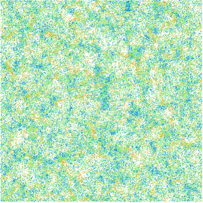
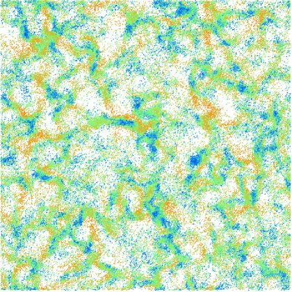
$t=40.96$ s, $C/N=670$ $t=446.6$ s, $C/N=5258$

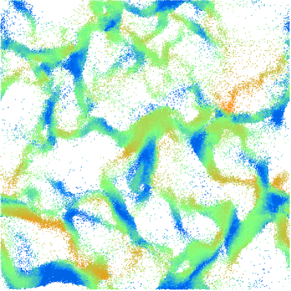
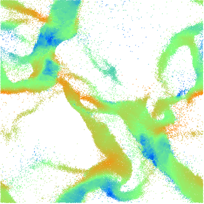
Figure 4: ED simulations with $N=79524$ particles in a system of length $L=500$ and volume fraction $\varrho=0.25$. The restitiution coefficient is $r=0.8$ and the critical collision frequency is $1/t_{c}=10^{5}$ s^-1. The energy of the single particles is color-coded according to the maximum (red), the mean (green), and the minimum (blue).

Density variations increase with time until, at long times, the size of the largest cluster is of order the system size. Snapshots of the system at different times are displayed, in that regime, in Fig. 4. The color codes the energy in the center of mass reference frame. Thus, different colors inside a cluster indicate either strong relative shear motion, expansion or compression. We note that a cluster does not behave like a solid body, but has internal motion and can eventually break into pieces after some time.

In Fig. 5 data from the same simulation are presented with a different color coding. Particles with a time between collisions smaller than $t_{c}$ can be seen mainly in the centers of the clusters colored in red. Note that most of the computational effort is spent in predicting collisions and to compute the velocities after the collisions. Therefore, the regions with the largest collision frequencies require the major part of the computational resources.

$t=40.96$ s, $C/N=670$ $t=446.6$ s, $C/N=5258$

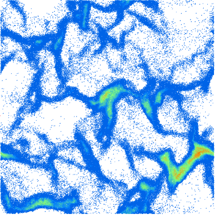
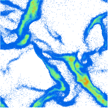
Figure 5: Collision frequency of individual particles from the simulation in Fig. 4. The colors indicate large (red), medium (green), and small (blue) collision frequencies.

An alternative color-coding of the same simulation allows us to view the mixing in the system. Particles with similar vertical coordinates are initially colored identically and keep their color in Fig. 6. At the upper and lower boundary, blue and red particles penetrate the others, respectively, due to the periodic boundaries. The shape of the initially flat boundary-interface between red and blue particles has strong contrast and is thus most evident. At sufficiently large times red and blue particles have travelled to the center of the system, and even later, inside the large clusters, one observes thin stripes of one color due to internal shear in the clusters. At the final stage, particles coming from different origin can be very close together at any point in the system due to the diffusive and ballistic mixing.

$t=40.96$ s, $C/N=670$ $t=446.6$ s, $C/N=5258$

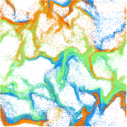
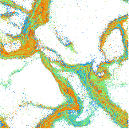
Figure 6: The particles from the simulation in Fig. 4 are initially colored corresponding to their vertical position and do not change their color.

5 Quantitative description of cluster growth

In order to describe the cluster growth more quantitatively, we propose a method to define clusters and to identify all the particles belonging to a specific cluster. Similar to the so-called “burning”-algorithm for percolation problems [30], our method identifies all particles that are in “contact” with each other. In contrast to the traditional method, that is applied to regular lattices where the sites are either occupied or not, our method works in the continuum and identifies particles that are in “contact”. Since we use perfectly rigid particles, we have to define contact in some arbitrary way. Two particles $i$ and $j$ with positions $\vec{r}_{i}$ and $\vec{r}_{j}$, and diameters $d_{i}$ and $d_{j}$, are assumed to be in contact if

$$|\vec{r}_{i}-\vec{r}_{j}|\leq S_{c}(d_{i}+d_{j})/2~{},$$ (6)

with the distance factor $S_{c}>1$. Consequently, all third particles $k$ for which the condition in Eq. (6) is true relative to particle $j$, are also in the same cluster as particle $i$, and so on.

For the identification of clusters, first, all particles are sorted into a “linked-cell” structure [28] what is convenient also for the simulation, and absolutely necessary for large particle numbers $N$ to avoid the numerical effort O$(N^{2})$ connected to nested loops of length $N$. The size of the cells is larger than the maximum of all $S_{c}(d_{i}+d_{j})/2$ here. From each cell starts a linked list that contains all particles with their center inside the cell. Now the criterion in Eq. (6) is tested for all particles $i$, but applied only to the particles $j$ in the same cell as $i$, or in the nearest-neighbor and next-nearest-neighbor cells.

The cluster identification algorithm starts with all particles $i$ being individual clusters of size $M_{i}=1$, stored in a linked list of length $i_{max}=N$, so that one has $N$ clusters at the beginning. Then, the distance between all particle pairs ($i$,$j$) that are close enough in the linked-cell structure is compared according to Eq. (6), but only if both particles belong to different clusters $i_{1}$ and $i_{2}$. If both particles are close enough, all particles from cluster $i_{2}$ are added to cluster $i_{1}$, while cluster $i_{2}$ is replaced by the last cluster $i_{max}$. At the same time, the number of clusters $i_{max}$ is reduced by one, so that the former cluster $i_{max}-1$ becomes the last one in the list. This is repeated until every pair ($i$,$j$) is examined once. If two particles belong already to the same cluster, one can proceed with the next pair, because no cluster merging is necessary.

After all pairs are examined, one has the size $M_{i}$ of every cluster $i$, the number of clusters $I_{c}=i_{max}$, the size of the largest cluster $M_{max}$, and the mean cluster size

$$\langle M\rangle=\frac{1}{I_{c}}\sum_{i=1}^{I_{c}}M_{i}~{}.$$ (7)

The size of a cluster is in this context the number of particles in it, and thus proportional to its mass, since we use mono-disperse particles. In Fig. 7 the quantities introduced above are displayed for the simulation in Figs. 3-6.

	Figure 7: (a) Number of clusters $I_{c}$ in the system from Figs. 3-6, plotted against time $t$, for different $S_{c}=1.05$, 1.1, 1.2, 1.3, and 1.4. (b) Mean cluster size $\langle M\rangle$ plotted against $t$. (c) Size of the largest cluster $M_{\rm max}$ plotted against $t$.

Since the parameter $S_{c}$ is arbitrary, we examine the simulation presented above for different $S_{c}$ values. The qualitative behavior is independent of $S_{c}$: (i) The number of clusters decreases with time, (ii) the mean cluster size grows correspondingly, and (iii) the largest cluster also grows in size during the simulation. In Figs. 7(a-c) it is easy to identify the three different regimes discussed above. In the homogeneous state, for times $t<1$ s, the change of $I_{c}$, $\langle M\rangle$, and $M_{\rm max}$ with time is very weak. At larger times, until about $t\approx 40$ s, the cluster growth regime is evidenced, and at very long times, one guesses a regime where $I_{c}$, $\langle M\rangle$, and $M_{\rm max}$ are again varying slowly.

Quantitatively, however, the behavior depends strongly on $S_{c}$. The larger $S_{c}$, the higher is the probability to find a particle $j$ that is close enough to a given particle $i$ so to be assumed as belonging to the same cluster. Only the maximum cluster size at large times is a quantity that becomes rather independent of $S_{c}$ for long enough times and small enough $S_{c}\leq 1.2$. This is because the regions outside the largest cluster are almost empty, so that a variation in $S_{c}$ has almost no effect. The few particles that hit the largest cluster are absorbed into it with high probability, so that it grows on and on.

The lines in Figs. 7(a,b) are fits of the cluster growth behavior to the laws

$$I_{c}\propto t^{-\cal M}{\rm~{}~{}and~{}}\langle M\rangle\propto t^{\cal M},$$ (8)

yielding the power ${\cal M}\approx 0.3$. Thus, the behavior of $I_{c}$ and $\langle M\rangle$ is described by one power with opposite sign. Unfortunately, the limited system size allows a reasonable fit only over a little more than one order of magnitude in time, so that the power law is a guess rather than a reliable functional behavior.

6 Summary and Conclusion

Simulations of freely cooling, two dimensional systems were presented. The behavior of the system was examined as a function of the restitution coefficient $r$ and the contact duration $t_{c}$. The system is initially in a homogeneous cooling state, and the deviations from this theoretically well understood situation occur earlier with stronger dissipation. The parameter that resembles a contact duration of the particle pairs is $t_{c}$ and has – varied over several orders of magnitude – only a weak effect on the behavior of the system, given that it is essentially smaller than the typical time between collisions.

When dissipation is strong enough, density variations build up and lead to clusters of particles. The deviation from the homogenous cooling state goes ahead with the growth of these formations. In order to quantify the cluster growth, we introduced a continuous “burning”-algorithm that allows to access e.g. the number of clusters in the system, the mean cluster size, and the size of the largest cluster. During the evolution of the system, the number of clusters decreases, and the mean cluster size increases correspondingly. The size of the maximum cluster also increases with time, and finally most particles in the system belong to the largest cluster.

The criterion to decide whether two particles belong to the same cluster or not, is based on the ratio of the interparticle distance and the particle size. Both the choice of this criterion and the magnitude of the distance factor $S_{c}$ are arbitrary. Alternatives would involve the collision frequency or the relative velocity of the particles under examination. However, we prefer the distance criterion for several reasons: (i) If $S_{c}$ is neither too small nor too large ($1.01\leq S_{c}\leq 1.2$ leads to reasonable results), the criterion accounts for nearest neighbors in a close packing, and particles that “feel” each other in the sense that a shear displacement would need a dilation of neighboring layers. (ii) The criterion is independent of the dimension (it is easily applied also to 3D situations – data not shown here), and (iii) the distance criterion can be applied to snapshots from a simulation, whereas other criteria might need more data and information. (iv) Finally, the distance criterion is independent of initial conditions like temperature, in contrast to a criterion that is based on the relative velocities of particles or on their collision frequencies.

We conclude that even about $10^{5}$ particles are not enough to examine the cluster growth regime over long enough times. Possibly, much larger simulations are necessary, in order to extend the available range in time. The presented large simulation was carried out on a small IBM 43P Power PC with 64 MB memory in several days of CPU time, so that a factor of at least 10 in the particle number should be possible with a faster computer. The event driven algorithm used is optimized for scalar machines, so that parallelization or vectorization are not feasible in the present state. However, there exist alternative schemes like the DSMC simulation method [31, 32, 25], which can be parallelized so that much larger particle numbers are accessible.

On the other hand, a more detailed parameter study, involving different collision models and possibly rotational degrees of freedom, might uncover parameter combinations with much slower cluster growth. The few simulations, we performed with different restitution coefficients and also with more realistic collision laws that couple to the rotational degrees of freedom [33], however, did not lead to remarkably different behavior. A more detailed parameter study and also the analysis of the cluster-size probability distribution in 2D and 3D are future perspectives requiring the use of a cluster-identification algorithm as proposed in this study.

References

- [1] R. P. Behringer and J. T. Jenkins, editors. Powders & Grains 97. Balkema, Rotterdam, 1997.
- [2] H. J. Herrmann, J.-P. Hovi, and S. Luding, editors. Physics of dry granular media - NATO ASI Series E 350. Kluwer Academic Publishers, Dordrecht, 1998.
- [3] I. Goldhirsch and G. Zanetti. Clustering instability in dissipative gases. Phys. Rev. Lett., 70(11):1619–1622, 1993.
- [4] S. McNamara and W. R. Young. Dynamics of a freely evolving, two-dimensional granular medium. Phys. Rev. E, 53(5):5089–5100, 1996.
- [5] S. Luding and S. McNamara. How to handle the inelastic collapse of a dissipative hard-sphere gas with the TC model. Granular Matter, 1(3):113–128, 1998. cond-mat/9810009.
- [6] J. J. Brey, J. W. Dufty, C. S. Kim, and A. Santos. Hydrodynamics for granular flow at low density. Phys. Rev. E, 58(4):4638, 1998.
- [7] B. Bernu and R. Mazighi. One-dimensional bounce of inelastically colliding marbles on a wall. J. Phys. A: Math. Gen., 23:5745, 1990.
- [8] S. McNamara and W. R. Young. Inelastic collapse and clumping in a one-dimensional granular medium. Phys. Fluids A, 4(3):496, 1992.
- [9] S. McNamara and W. R. Young. Kinetics of a one-dimensional granular medium in the quasielastic limit. Phys. Fluids A, 5(1):34, 1993.
- [10] S. Luding, E. Clément, A. Blumen, J. Rajchenbach, and J. Duran. Studies of columns of beads under external vibrations. Phys. Rev. E, 49(2):1634, 1994.
- [11] E. L. Grossman and B. Roman. Density variations in a one-dimensional granular system. Phys. Fluids, 8:3218, 1996.
- [12] A. Kudrolli and J. P. Gollub. Studies of cluster formation due to collisions in granular material. In Powders & Grains 97, page 535, Rotterdam, 1997. Balkema.
- [13] A. Kudrolli, M. Wolpert, and J.P. Gollub. Cluster formation due to collisions in granular material. Phys. Rev. Lett., 78(7):1383–1386, 1997.
- [14] M. Sibuya, T. Kawai, and K. Shida. Equipartition of particles forming clusters by inelastic collisions. Physica A, 167:676, 1990.
- [15] S. McNamara and W. R. Young. Inelastic collapse in two dimensions. Phys. Rev. E, 50(1):R28–R31, 1994.
- [16] E. Trizac and J. P. Hansen. Dynamic scaling behavior of ballistic coalescence. Phys. Rev. Lett., 74(21):4114–4117, 1995.
- [17] F. Spahn, U. Schwarz, and J. Kurths. Clustering of granular assemblies with temperature dependent restitution and under keplerian differential rotation. Phys. Rev. Lett., 78:1596–1599, 1997.
- [18] P. Deltour and J.-L. Barrat. Quantitative study of a freely cooling granular medium. J. Phys. I France, 7:137–151, 1997.
- [19] J. A. G. Orza, R. Brito, T. P. C. van Noije, and M. H. Ernst. Patterns and long range correlations in idealized granular flows. Int. J. of Mod. Phys. C, 8:953, 1997.
- [20] J. S. Olafsen and J. S. Urbach. Clustering, order and collapse in a driven granular monolayer. Phys. Rev. Lett., 81:4369, 1998. cond-mat/9807148.
- [21] P. K. Haff. Grain flow as a fluid-mechanical phenomenon. J. Fluid Mech., 134:401–430, 1983.
- [22] S. B. Savage. Gravity flow of cohesionless granular materials in chutes and channels. J. Fluid Mech., 92:53, 1979.
- [23] J. T. Jenkins and S. C. Cowin. Theories for flowing granular materials. In S. C. Cowin, editor, Mechanics Applied to the Transport of Bulk Materials, New York, 1979. Am. Soc. Mech. Eng.
- [24] R. Brito and M. H. Ernst. Extension of Haff’s cooling law in granular flows. cond-mat/9807224, 1998.
- [25] S. Luding. Clustering instabilities, arching, and anomalous interaction probabilities as examples for cooperative phenomena in dry granular media. T.A.S.K. Quarterly, Scientific Bulletin of Academic Computer Centre of the Technical University of Gdansk, 2(3):417–443, July, 1998.
- [26] S. Luding, E. Clément, J. Rajchenbach, and J. Duran. Simulations of pattern formation in vibrated granular media. Europhys. Lett., 36(4):247–252, 1996.
- [27] S. Luding. Surface waves and pattern formation in vibrated granular media. In Powders & Grains 97, pages 373–376, Amsterdam, 1997. Balkema.
- [28] M. P. Allen and D. J. Tildesley. Computer Simulation of Liquids. Oxford University Press, Oxford, 1987.
- [29] S. Luding, M. Huthmann, S. McNamara, and A. Zippelius. Homogeneous cooling of rough dissipative particles: Theory and simulations. Phys. Rev. E, 58:3416–3425, 1998.
- [30] H. J. Herrmann, D. C. Hong, and H. E. Stanley. Backbone and elastic backbone of percolation clusters obtained by the new method of ‘burning’. J. Phys. A, 17:L261, 1984.
- [31] M. Müller, S. Luding, and H. J. Herrmann. Simulations of vibrated granular media in 2d and 3d. In D. E. Wolf and P. Grassberger, editors, Friction, Arching and Contact Dynamics, Singapore, 1997. World Scientific.
- [32] S. Luding, M. Müller, and S. McNamara. The validity of “molecular chaos” in granular flows. In World Congress on Particle Technology, Davis Building, 165-189 Railway Terrace, Rugby CV21 3HQ, UK, 1998. Institution of Chemical Engineers. ISBN 0-85295-401-9.
- [33] S. Luding. Collisions & contacts between two particles. In H. J. Herrmann, J.-P. Hovi, and S. Luding, editors, Physics of dry granular media - NATO ASI Series E350, page 285, Dordrecht, 1998. Kluwer Academic Publishers.