Abstract

Granular media are examined with the focus on polydisperse mixtures in the presence of two localized heat-baths. If the two driving energies are similar, the large particles prefer to stay in the ‘cold’ regions of the system – as far away from the energy source as possible. If one of the temperatures is larger than the other, the cold region is shifted towards the colder reservoir; if the temperature of one source is much higher, a strong, almost constant temperature gradient builds up between the two reservoirs and the large particles are found close to the cold reservoir. Furthermore, clustering is observed between the heat reservoirs, if dissipation is strong enough.

1 Introduction

The segregation of granular materials is an effect of eminent importance for industrial operations and has been a subject of research for decades. The behavior of powders within the industrial environment, e.g. silos, hoppers, conveyor belts or chutes, displays interesting effects - one of them is size segregation. Segregation or the mixing properties of granular media are not yet completely understood and thus cannot be controlled under all circumstances. For a review of experimental techniques, theoretical approaches, and numerical simulations see Refs. [1, 2] and the references therein.

A lot of effort has been invested in the understanding of size-segregation (see this proceedings for a recent overview of the state of the art). It turns out that segregation can be driven by geometric effects, shear, percolation and also by a convective motion of the small particles in the system [3]. Segregation due to convection, in rather dilute, more dynamic systems appears to be orders of magnitude faster than segregation due to purely geometrical effects in dense, quasi-static situations [4, 5]. However, there are still a lot of open questions which are subject to current research on model granular media [6, 7, 8, 1, 9].

Most of the segregation phenomena are obtained in the presence of gradients in density or temperature. Here we isolate the latter case, i.e. we examine the segregation of two species of grains in the presence of local heat reservoirs, but in the absence of external forces like e.g. gravity.

2 The inelastic hard sphere model

In this study, we use the standard interaction model for the instantaneous collisions of particles with radii $a_{k}$, and mass $m_{k}$, with the subscripts $k=S$ or $L$, for small and large particles, respectively. This model accounts for dissipation, using the restitution coefficient $r$, and is introduced and discussed in more detail in Refs. [10, 11, 12, 13, 9]. The post-collisional velocities ${\mathbf{v}}^{\prime}$ are given in terms of the pre-collisional velocities ${\mathbf{v}}$ by

$${\mathbf{v}}_{1,2}^{\prime} = {\mathbf{v}}_{1,2}\mp\frac{(1+r)~{}m_{\rm red}}{m_{1,2}}{\mathbf{v}}_{n}~{},$$ (1)

with ${\mathbf{v}}_{n}\equiv\left[({\mathbf{v}}_{1}-{\mathbf{v}}_{2})\cdot{\mathbf{v}}_{n}\right]{\mathbf{\hat{}}n}$, the normal component of ${\mathbf{v}}_{1}-{\mathbf{v}}_{2}$, parallel to ${\mathbf{\hat{}}n}$, the unit vector pointing along the line connecting the centers of the colliding particles. The reduced mass is here $m_{\rm red}=m_{1}m_{2}/(m_{1}+m_{2})$. If two particles collide, their velocities are changed according to Eq. (1).

If a particle $i$ crosses a line of fixed temperature $T_{j}$, its velocity is changed in magnitude, but not in direction, according to the rule

$${\mathbf{v}}_{i}^{\prime}=\pm v^{T_{j}}\frac{{\mathbf{v}}_{i}}{|{\mathbf{v}}_{i}|}~{},$$ (2)

with the random thermal velocity $\pm v^{T_{j}}$ drawn from a Maxwellian velocity distribution, and with random sign. (If the ‘$+$’ sign is used in Eq. (2), a large net mass flux occurs when a cluster of particles crosses a line of fixed temperature. If the ‘$-$’ sign is used the two subsystems have conserved particle numbers, but are still coupled via collisions across the boundaries.) In 2D one has $v^{T_{j}}=\sqrt{v_{x}^{2}+v_{y}^{2}}~{}$, where $v_{x}$ and $v_{y}$ are the components of the thermal velocity vector, each distributed according to a Gaussian distribution. Eq. (2) is also applied to particles after a collision, if the particle’s center of mass is closer than $a_{L}$ to one of the heat reservoirs $j$.

In order to obtain the two random velocities $v_{x}$ and $v_{y}$, two random numbers $r_{1}$ and $r_{2}$, homogeneously distributed in the interval $[0:1]$ are used. With the desired typical thermal velocity $\bar{v}=\sqrt{2T_{j}/m_{i}}$, one has

$$v_{x}=\sqrt{-\bar{v}^{2}\ln r_{2}}\cos(2\pi r_{1})~{},{\rm~{}and~{}}$$ (3)

$$v_{y}=\sqrt{-\bar{v}^{2}\ln r_{2}}\sin(2\pi r_{1})~{},~{}~{}~{}~{}~{}~{}~{}$$ (4)

using the method by Box and Muller, as described in Ref. [14].

If the velocity of the particle would be set to ${\bf v}^{\prime}=(v_{x},v_{y})$, artificial peaks in the density at the positions $Z_{1}$ and $Z_{2}$ would be observed. This artefact was the reason to choose the above described way of thermal coupling. Note, that our coupling to a reservoir does not guarantee a certain temperature in a small volume around the reservoir [15, 16]. It rather adjusts the velocity of all particles that came along the reservoir and touched it with their center of mass. Those particles which approach the reservoir usually have a lower temperature and thus reduce the mean. As $r$ decreases, the reduction increases. Our choice of thermal coupling is arbitrary, however, the discussion of thermostating is far from the scope of the present paper – therefore, we restrict ourselves to the method introduced here.

Our method of imposing a temperature gradient does not have any simple physical analog, but it does allow us to isolate the effects of the temperature gradient. More physically feasible energy sources, such as vibrating walls perturb the motion more than the method used here.

3 The event-driven simulation method

For the simulation of the hard spheres, we use the event-driven algorithm, originally introduced by Lubachevsky [17], and applied to the simulation of granular media e.g. in Refs. [13]. In these simulations, the particles follow an undisturbed translational motion until an event occurs. An event is either the collision of two particles, the crossing of one particle with the boundary of a cell (in the linked-cell structure which is used for algorithmic optimization only), or the crossing of one of the lines with fixed temperature. A particle-particle collision is treated as described in the previous section, a cell-boundary crossing has no effect on the particle-motion, and the crossing of a fixed temperature location leads to a change of velocity according to Eq. (2). Only the particle(s) involved in the last event is (are) treated and their next event is computed. In the next step (which does not imply a fixed step in time), the next event out of all possible events is treated.

4 Boundary conditions and system parameters

$r=1.0$ $r=0.95$

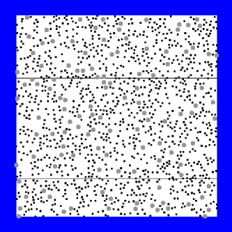
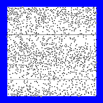
$r=0.90$ $r=0.60$

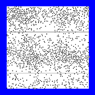
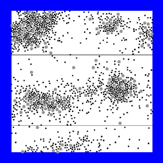
Figure 1.  : Snapshots from different simulations with $r=1.0$, 0.95, 0.90, and 0.60. The heat reservoirs are indicated by horizontal lines; the large particles are displayed in light grey, the small in black.

The simulations presented here (typical situations are displayed in Fig. 1) were performed with $N=1296$ particles in a two-dimensional (2D) box of size $l=l_{x}=l_{y}=0.04$ m. The box has periodic boundaries, i.e. a particle that leaves the volume at the bottom (left), immediately enters it at the top (right) and vice-versa. Two particle types ($S$, $L$) are used with $a_{S}=a=2.5\times 10^{-4}$ m and $a_{L}=2a=5\times 10^{-4}$ m. In the system with dimensionless size $L=l/a=80$, $N_{S}=1176$ particles of the small species and $N_{L}=120$ particles of the large species coexist. Note that we used a rather arbitrary choice for the calculation of the particle mass (see above) so that $m_{L}=8m_{S}$ for the size ratio used here. The fraction of the area which is occupied by the particles, i.e. the total volume fraction, is $\nu=\pi(N_{S}a_{S}^{2}+N_{L}a_{L}^{2})/l^{2}\approx 0.2$.

The hot and cold temperature reservoirs are situated at the vertical positions $Z_{2}=z_{2}/a=15$ and $Z_{1}=z_{1}/a=55$, respectively, and reach over the whole width of the system. The temperatures of the reservoirs are $T_{1}$ and $T_{2}$ – but since no external body force like gravity is involved the behavior of the system does not depend on the absolute value of $T_{1}$ or $T_{2}$; only the ratio $T_{2}/T_{1}$ is important, and it is varied in the range from $T_{2}/T_{1}=1$ to 9 in the following. In Fig. 1 snapshots of simulations with $T_{2}/T_{1}=1$ and different values of $r$ are plotted. For small $r$, clustering is observed and the averaging over horizontal slices (data are presented in Fig. 2) becomes questionable.

Figure 2.  : Density $\rho$ (top) and temperature $\tau$ (bottom), plotted as function of the vertical position in the system $Z=z/a$. Data for small (Left) and large (Right) particles are presented for $T_{2}/T_{1}=1$ and different restitution coefficients $r$ as given in the inset. The data at $z/a=0$ and $z/a=80$ are identical due to periodic boundaries.

5 Results

A quantitative measure of segregation is the partial density of the different species. We present $\rho_{k}=n_{k}/N_{k}$, the particle number density $n_{k}(z)$ weighed by the number of particles $N_{k}$ of species $k$ in Fig. 2. The strength of segregation increases with decreasing $r$, only for small $r=0.60$, segregation is rather weak due to clustering. Fluctuations in density are correlated to the heat reservoirs: Close to a “hot” region in the vicinity of a energy source, the density is lower than in the “cold” regions in between. Note that the large particles segregate, while the small particles make up a “background fluid” with a comparatively small density variation, if dissipation is weak. Thus, all particles prefer regions of low temperature, but the large ones are attracted by the cold regions more strongly.

Figure 3.  : Density $\rho$ (top) and temperature $\tau$ (bottom), plotted as function of the vertical position in the system $Z=z/a$. Data for small (Left) and large (Right) particles are presented for $r=0.99$ and different temperature ratios $T_{2}/T_{1}$.

Now, the restitution coefficient is fixed to $r=0.99$ and the temperature ratio $T_{2}/T_{1}$ is modified. In Fig. 3 the situation is presented for different ratios $T_{2}/T_{1}=1$, 2, 3, 5, and 9. The large particles segregate from the “background fluid” made up by the small particles and the quality of segregation increases with the magnitude of the temperature gradient. For $T_{2}>T_{1}$ the large (and heavier) particles can be found close to the colder heat reservoir, as different to the situation discussed above. When heavier particles have the same temperature as light ones, their mean velocity is reduced, so that they can not diffuse away from the cold heat reservoir.

6 Summary and Conclusion

In summary, we presented simulations of different size particles in the presence of a temperature gradient. If the temperature gradient is due to the dissipative nature of the material, the large particles move towards the cold regions, as far away from an energy source as possible. If the gradient in temperature is externally imposed, most of the large particles prefer to move towards the colder heat reservoir. When dissipation is strong enough, clustering is observed in the locally driven system.

Further possible studies involve the prediction of the density and temperature profiles with kinetic theory – first for the monodisperse and later also for the polydisperse case.

References

- [1] Physics of dry granular media - NATO ASI Series E 350, edited by H. J. Herrmann, J.-P. Hovi, and S. Luding (Kluwer Academic Publishers, Dordrecht, 1998).
- [2] Z. T. Chowhan, Pharm. Technol. 19, 56 (1995).
- [3] J. B. Knight, H. M. Jaeger, and S. R. Nagel, Phys. Rev. Lett. 70, 3728 (1993).
- [4] J. Duran, T. Mazozi, E. Clément, and J. Rajchenbach, Phys. Rev. E 50, 5138 (1994).
- [5] S. Dippel and S. Luding, J. Phys. I France 5, 1527 (1995).
- [6] A. D. Rosato, K. J. Strandburg, F. Prinz, and R. H. Swendsen, Phys. Rev. Lett. 58, 1038 (1987).
- [7] E. Clément, J. Rajchenbach, and J. Duran, Europhys.Lett. 30, 7 (1995).
- [8] F. Cantelaube, Y. L. Duparcmeur, D. Bideau, and G. H. Ristow, J. Phys. I France 5, 581 (1995).
- [9] B. Arnarson and J. T. Willits, Phys. Fluids 10, 1324 (1998).
- [10] J. T. Jenkins and M. W. Richman, Phys. of Fluids 28, 3485 (1985).
- [11] C. K. K. Lun, J. Fluid Mech. 233, 539 (1991).
- [12] A. Goldshtein and M. Shapiro, J. Fluid Mech. 282, 75 (1995).
- [13] S. Luding, M. Huthmann, S. McNamara, and A. Zippelius, Phys. Rev. E 58, 3416 (1998).
- [14] W. H. Press, S. A. Teukolsky, W. T. Vetterling, and B. P. Flannery, Numerical Recipes (Cambridge University Press, Cambridge, 1992).
- [15] P. J. Cause and M. Mareschal, Phys Rev A 38, 4241 (1988).
- [16] M. Mareschal, M. Monsour, G. Sonnino, and E. Kestamont, Phys Rev A 45, 7180 (1992).
- [17] B. D. Lubachevsky, J. of Comp. Phys. 94, 255 (1991).