Density Matrix Renormalization

Abstract

The Density Matrix Renormalization Group (DMRG) has become a powerful numerical method that can be applied to low-dimensional strongly correlated fermionic and bosonic systems. It allows for a very precise calculation of static, dynamic and thermodynamic properties. Its field of applicability has now extended beyond Condensed Matter, and is successfully used in Statistical Mechanics and High Energy Physics as well. In this article, we briefly review the main aspects of the method. We also comment on some of the most relevant applications so as to give an overview on the scope and possibilities of DMRG and mention the most important extensions of the method such as the calculation of dynamical properties, the application to classical systems, inclusion of temperature, phonons and disorder and a recent modification for the ab initio calculation of electronic states in molecules.

1 Introduction

The basics of the Density Matrix Renormalization Group were developed by S. White in 1992[1] and since then DMRG has proved to be a very powerful method for low dimensional interacting systems. Its remarkable accuracy can be seen for example in the spin-1 Heisenberg chain: for a system of hundreds of sites a precision of $10^{-10}$ for the ground state energy can be achieved. Since then it has been applied to a great variety of systems and problems (principally in one dimension) including, among others, spin chains, fermionic and bosonic systems, disordered models, impurities, etc. It has also been improved substantially in several directions like two dimensional (2D) classical systems, phonons, molecules, the inclusion of temperature and the calculation of dynamical properties. Some calculations have also been performed in 2D quantum systems. All these topics are treated in detail and in a pedagogical way in a book published recently, where the reader can find an extensive review on DMRG[2].

In this article we will attempt to cover the different areas where it has been applied. Regretfully, however, we won’t be able to review the large number of papers that have been written using different aspects of this very efficient method. We have chosen what, in our opinion, are the most representative contributions and we suggest the interested reader to look for further information in these references. Our aim here is to give the reader a general overview on the subject.

One of the most important limitations of numerical calculations in finite systems is the great amount of states that have to be considered and its exponential growth with system size. Several methods have been introduced in order to reduce the size of the Hilbert space to be able to reach larger systems, such as Monte Carlo, renormalization group (RG) and DMRG. Each method considers a particular criterion to keep the relevant information.

The DMRG was originally developed to overcome the problems that arise in interacting systems in 1D when standard RG procedures were applied. Consider a block B (a block is a collection of sites) where the Hamiltonian $H_{B}$ and end-operators are defined. These traditional methods consist in putting together two or more blocks (e.g. B-B’, which we will call the superblock), connected using end-operators, in a basis that is a direct product of the basis of each block, forming $H_{BB^{\prime}}$. This Hamiltonian is then diagonalized, the superblock is replaced by a new effective block $B_{new}$ formed by a certain number $m$ of lowest-lying eigenstates of $H_{BB^{\prime}}$ and the iteration is continued (see Ref. [3]). Although it has been used successfully in certain cases, this procedure, or similar versions of it, has been applied to several interacting systems with poor performance. For example, it has been applied to the 1D Hubbard model keeping $m\simeq 1000$ states. For 16 sites, an error of 5-10% was obtained [4]. Other results[5] were also discouraging. A better performance was obtained [6] by adding a single site at a time rather than doubling the block size. However, there is one case where a similar version of this method applies very well: the Kondo model. Wilson[7] mapped the one-impurity problem onto a one-dimensional lattice with exponentially descreasing hoppings. The difference with the method explained above is that in this case, one site (equivalent to an “onion shell”) is added at each step and, due to the exponential decrease of the hopping, very accurate results can be obtained.

Returning to the problem of putting several blocks together, the main source of error comes from the election of eigenstates of $H_{BB^{\prime}}$ as representative states of a superblock. Since $H_{BB^{\prime}}$ has no connection to the rest of the lattice, its eigenstates may have unwanted features (like nodes) at the ends of the block and this can’t be improved by increasing the number of states kept. Based on this consideration, Noack and White[8] tried including different boundary conditions and boundary strengths. This turned out to work well for single particle and Anderson localization problems but, however, it did not improve significantly results in interacting systems. These considerations lead to the idea of taking a larger superblock that includes the blocks $BB^{\prime}$, diagonalize the Hamiltonian in this large superblock and then somehow project the most favorable states onto $BB^{\prime}$. Then $BB^{\prime}$ is replaced by $B_{new}$. In this way, awkward features in the boundary would vanish and a better representation of the states in the infinite system would be achieved. White[1, 3] proposed the density matrix as the optimal way of projecting the best states onto part of the system and this will be discussed in the next section. The justification of using the density matrix is given in detail in Ref.[2]. A very easy and pedagogical way of understanding the basic functioning of DMRG is applying it to the calculation of simple quantum problems like one particle in a tight binding chain [9, 10].

In the following Section we will briefly describe the standard method; in Sect. 3 we will mention some of the most important applications; in Sect. 4 we review the most relevant extensions to the method and finally in Sect. 5 we concentrate on the way dynamical calculations can be performed within DMRG.

2 The Method

The DMRG allows for a systematic truncation of the Hilbert space by keeping the most probable states describing a wave function (e.g. the ground state) instead of the lowest energy states usually kept in previous real space renormalization techniques.

The basic idea consists in starting from a small system (e.g with $N$ sites) and then gradually increase its size (to $N+2$, $N+4$,…) until the desired length is reached. Let us call the collection of $N$ sites the universe and divide it into two parts: the system and the environment (see Fig. 1). The Hamiltonian is constructed in the universe and its ground state $|\psi_{0}>$ is obtained. This is considered as the state of the universe and called the target state. It has components on the system and the envorinment. We want to obtain the most relevant states of the system, i.e., the states of the system that have largest weight in $|\psi_{0}\rangle$. To obtain this, the environment is considered as a statistical bath and the density matrix[11] is used to obtain the desired information on the system. So instead of keeping eigenstates of the Hamiltonian in the block (system), we keep eigenstates of the density matrix. We will be more explicit below.

Figure 1: A scheme of the superblock (universe) configuration for the DMRG algorithm[3].

Let’s define block [B] as a finite chain with $l$ sites, having an associated Hilbert space with $m$ states where operators are defined (in particular the Hamiltonian in this finite chain, $H_{B}$ and the operators at the ends of the block, useful for linking it to other chains or added sites). Except for the first iteration, the basis in this block isn’t explicitly known due to previous basis rotations and reductions. The operators in this basis are matrices and the basis states are characterized by quantum numbers (like $S^{z}$, charge or number of particles, etc). We also define an added block or site as [a] having $n$ states.

A general iteration of the method consists of:

i) Define the Hamiltonian $H_{BB^{\prime}}$ for the superblock (the universe) formed by putting together two blocks [B] and [B’] and two added sites [a] and [a’] in this way: [B a a’ B’ ] (the primes are only to indicate additional blocks, but the primed blocks have the same structure as the non-primed ones; this can vary, see the finite size algorithm below). In general, blocks [B] and [B’] come from the previous iteration. The total Hilbert space of this superblock is the direct product of the individual spaces corresponding to each block and the added sites. In practice a quantum number of the superblock can be fixed (in a spin chain for example one can look at the total $S^{z}=0$ subspace), so the total number of states in the superblock is much smaller than $(mn)^{2}$. As, in some cases, the quantum number of the superblock consists of the sum of the quantum numbers of the individual blocks, each one must contain several subspaces (several values of $S^{z}$ for example).

Here periodic boundary conditions can be attached to the ends and a different block layout should be considered (e.g. [B a B’ a’ ]) to avoid connecting blocks [B] and [B’] which takes longer to converge. The boundary conditions are between [a’] and [B]. For closed chains the performance is poorer than for open boundary conditions [3].

ii) Diagonalize the Hamiltonian $H_{BB^{\prime}}$ to obtain the ground state $|\psi_{0}\rangle$ (target state) using Lanczos[12] or Davidson[13] algorithms. Other states could also be kept, such as the first excited ones: they are all called target states.

iii) Construct the density matrix:

$$\rho_{ii^{\prime}}=\sum_{j}\psi_{0,ij}\psi_{0,i^{\prime}j}$$ (1)

on block [B a], where $\psi_{0,ij}=\langle i\otimes j|\psi_{0}\rangle$, the states $|i\rangle$ belonging to the Hilbert space of the block [B a] and the states $|j\rangle$ to the block [B’ a’]. The density matrix considers the part [B a] as a system and [B’ a’], as a statistical bath. The eigenstates of $\rho$ with the highest eigenvalues correspond to the most probable states (or equivalently the states with highest weight) of block [B a] in the ground state of the whole superblock. These states are kept up to a certain cutoff, keeping a total of $m$ states per block. The density matrix eigenvalues sum up to unity and the truncation error, defined as the sum of the density matrix eigenvalues corresponding to discarded eigenvectors, gives a qualitative indication of the accuracy of the calculation.

iv) With these $m$ states a rectangular matrix $O$ is formed and it is used to change basis and reduce all operators defined in [B a]. This block [B a] is then renamed as block [B_new] or simply [B] (for example, the Hamiltonian in block [B a], $H_{Ba}$, is transformed into $H_{B}$ as $H_{B}=O^{\dagger}H_{Ba}O$).

v) A new block [a] is added (one site in our case) and the new superblock [B a a’ B’] is formed as the direct product of the states of all the blocks.

vi) This iteration continues until the desired length is achieved. At each step the length is $N=2l+2$ (if [a] consists of one site).

When more than one target state is used, i.e more than one state is wished to be well described, the density matrix is defined as:

$$\rho_{ii^{\prime}}=\sum_{l}p_{l}\sum_{j}\phi_{l,ij}\phi_{l,i^{\prime}j}$$ (2)

where $p_{l}$ defines the probability of finding the system in the target state $|\phi_{l}\rangle$ (not necessarily eigenstates of the Hamiltonian).

The method described above is usually called the infinite system algorithm since the system size increases in two lattice sites (if the added block [a] has one site) at each iteration. There is a way to increase precision at each length $N$ called the finite system algorithm. It consists of fixing the lattice size and zipping a couple of times until convergence is reached. In this case and for the block configuration [B a a’ B’ ], $N=l+1+1+l^{\prime}$ where $l$ and $l^{\prime}$ are the number of sites in $B$ and $B^{\prime}$ respectively. In this step the density matrix is used to project onto the left $l+1$ sites. In order to keep $N$ fixed, in the next block configuration, the right block $B^{\prime}$ should be defined in $l-1$ sites such that $N=(l+1)+1+1+(l-1)^{\prime}$. The operators in this smaller block should be kept from previous iterations (in some cases from the iterations for the system size with $N-2$)[2].

The calculation of static properties like correlation functions is easily done by keeping the operators in question at each step and performing the corresponding basis change and reduction, in a similar manner as done with the Hamiltonian in each block[3]. The energy and measurements are calculated in the superblock. A faster convergence of Lanczos or Davidson algorithm is achieved by choosing a good trial vector[14, 15]. An interesting analysis on DMRG accuracy is done in Ref. [16]. Fixed points of the DMRG and their relation to matrix product wave functions were studied in [17] and an analytic formulation combining the block renormalization group with variational and Fokker-Planck methods in [18]. The connection of the method with quantum groups and conformal field theory is treated in [19]. There are also interesting connections between the density matrix spectra and integrable models[20] via corner transfer matrices. These articles give a deep insight into the essence of the DMRG method.

3 Applications

Since its development, the number of papers using DMRG has grown enormously and other improvements to the method have been performed. We would like to mention some applications where this method has proved to be useful. Other applications related to further developments of the DMRG will be mentioned in Sect. 4.

A very impressive result with unprecedented accuracy was obtained by White and Huse [21] when calculating the spin gap in a $S=1$ Heisenberg chain obtaining $\Delta=0.41050J$. They also calculated very accurate spin correlation functions and excitation energies for one and several magnon states and performed a very detailed analysis of the excitations for different momenta. They obtained a spin correlation length of 6.03 lattice spacings. Simultaneously Sørensen and Affleck[22] also calculated the structure factor and spin gap for this system up to length 100 with very high accuracy, comparing their results with the nonlinear $\sigma$ model. In a subsequent paper[23] they applied the DMRG to the anisotropic $S=1$ chain, obtaining the values for the Haldane gap. They also performed a detailed study of the $S=1/2$ end excitations in an open chain. Thermodynamic properties in open $S=1$ chains such as specific heat, electron paramagnetic resonance (EPR) and magnetic susceptibility calculated using DMRG gave an excellent fit to experimental data, confirming the existence of free spins 1/2 at the boundaries[24]. A related problem, i.e. the effect of non-magnetic impurities in spin systems (dimerized, ladders and 2D) was studied in [25].

For larger integer spins there have also been some studies. Nishiyama and coworkers[26] calculated the low energy spectrum and correlation functions of the $S=2$ antiferromagnetic Heisenberg open chain. They found $S=1$ end excitations (in agreement with the Valence Bond Theory). Edge excitations for other values of $S$ have been studied in Ref. [27]. Almost at the same time Schollwöck and Jolicoeur[28] calculated the spin gap in the same system, up to 350 sites, ($\Delta=0.085J$), correlation functions that showed topological order and a spin correlation length of 49 lattice spacings. More recent accurate studies of $S=2$ chains are found in [29, 30]. In Ref. [31] the dispersion of the single magnon band and other properties of the $S=2$ antiferromagnetic Heisenberg chains were calculated.

Concerning $S=1/2$ systems, DMRG has been crucial for obtaining the logarithmic corrections to the $1/r$ dependence of the spin-spin correlation functions in the isotropic Heisenberg model [32]. For this, very accurate values for the energy and correlation functions were needed. For $N=100$ sites an error of $10^{-5}$ was achieved keeping $m=150$ states per block, comparing with the exact finite-size Bethe Ansatz results. For this model it was found that the data for the correlation function has a very accurate scaling behaviour and advantage of this was taken to obtain the logarithmic corrections in the thermodynamic limit. Other calculations of the spin correlations have been performed for the anisotropic case [33].

Similar calculations have been performed for the $S=3/2$ Heisenberg chain [34]. In this case a stronger logarithmic correction to the spin correlation function was found. For this model there was interest in obtaining the central charge $c$ to elucidate whether this model corresponds to the same universality class as the $S=1/2$ case, where the central charge can be obtained from the finite-size scaling of the energy. Although there have been previous attempts[35], these calculations presented difficulties since they involved also a term $\sim 1/\ln^{3}N$. With the DMRG the value $c=1$ was clearly obtained.

In Ref. [36], DMRG was applied to an effective spin Hamiltonian obtained from an SU(4) spin-orbit critical state in 1D. Another application to enlarged symmetry cases (SU(4)) was done to study coherence in arrays of quantum dots[37].

Dimerization and frustration have been considered in Refs. [38, 39, 40, 41, 42, 43, 44, 45] and alternating spin chains in [46]. The case of several coupled spin chains (ladder models) [47], magnetization properties and plateaus for quantum spin ladder systems[48] and finite 2D systems like an application to $CaV_{4}O_{9}$ reaching 24x11 square lattices [14] have also been studied.

There has been a great amount of applications to fermionic systems such as 1D Hubbard and t-J models [49]. Also several coupled chains at different dopings have been considered [50]. Quite large systems can be reached, for example in [51], a 4x20 lattice was considered to study ferromagnetism in the infinite U Hubbard model; the ground state of a 4-leg t-J ladder in [52]; the one and two hole ground state in a 10x7 t-J lattice[53]; a doped 3-leg t-J ladder[54] and the study of striped phases and domain walls in 19x8 t-J systems[55]. Impurity problems have been studied for example in one- [56] and two-impurity [57] Kondo systems, Kondo and Anderson lattices [58, 59, 60], Kondo lattices with localized $f^{2}$ configurations[61], a t-J chain coupled to localized Kondo spins[62] and ferromagnetic Kondo models for manganites [63].

4 Other extensions to DMRG

There have been several extensions to DMRG like the inclusion of symmetries to the method such as spin and parity[64, 65]. Total spin conservation and continuous symmetries have been treated in [66] and in interaction-round a face Hamiltonians[67], a formulation that can be applied to rotational-invariant sytems like $S=1$ and 2 chains[30]. A momentum representation of this technique [68] that allows for a diagonalization in a fixed momentum subspace has been developed as well as applications in dimension higher than one[14, 69] and Bethe lattices[70]. The inclusion of symmetries is essential to the method since it allows to consider a smaller number of states, enhance precision and obtain eigenstates with a definite quantum number.

Other recent applications have been in nuclear shell model calculations where a two level pairing model has been considered[71] and in the study of ultrasmall superconducting grains, in this case, using the particle (hole) states around the Fermi level as the system (environment) block[72].

A very interesting and successful application is a recent work in High Energy Physics[73]. Here the DMRG is used in an asymptotically free model with bound states, a toy model for quantum chromodynamics, namely the two dimensional delta-function potential. For this case an algorithm similar to the momentum space DMRG[68] was used where the block and environment consist of low and high energy states respectively. The results obtained here are much more accurate than the similarity renormalization group[74] and a generalization to field-theoretical models is proposed based on the discreet light-cone quantization in momentum space[75].

Below we briefly mention other important extensions, leaving the calculation of dynamical properties for the next Section.

4.1 Classical systems

The DMRG has been very successfully extended to study classical systems. For a detailed description we refer the reader to Ref. [76]. Since 1D quantum systems are related to 2D classical systems[77], it is natural to adapt DMRG to the classical 2D case. This method is based on the renormalization group transformation for the transfer matrix $T$. It is a variational method that maximizes the partition function using a limited number of degrees of freedom, where the variational state is written as a product of local matrices[17]. For 2D classical systems, this algorithm is superior to the classical Monte Carlo method in accuracy, speed and in the possibility of treating much larger systems.

A further improvement to this method is based on the corner transfer matrix[78], the CTMRG[79] and can be generalized to any dimension[80].

It was first applied to the Ising model[76, 81] and also to the Potts model[82], where very accurate density profiles and critical indices were calculated. Further applications have included non-hermitian problems in equilibrium and non-equilibrium physics. In the first case, transfer matrices may be non-hermitian and several situations have been considered: a model for the Quantum Hall effect[83] and the $q$-symmetric Heisenberg chain related to the conformal series of critical models[84]. In the second case, the adaptation of the DMRG to non-equilibrium physics like the asymmetric exclusion problem[85] and reaction-diffusion problems [86, 87] has shown to be very successful.

4.2 Finite temperature DMRG

The adaptation of the DMRG method for classical systems paved the way for the study of 1D quantum systems at non zero temperature, by using the Trotter-Suzuki method [88, 89, 90, 91]. In this case the system is infinite and the finiteness is in the level of the Trotter approximation. Standard DMRG usually produces its best results for the ground state energy and less accurate results for higher excitations. A different situation occurs here: the lower the temperature, the less accurate the results.

Very nice results have been obtained for the dimerized, $S=1/2$, XY model, where the specific heat was calculated involving an extremely small basis set[88] ($m=16$), the agreement with the exact solution being much better in the case where the system has a substantial gap.

It has also been used to calculate thermodynamic properties of the anisotropic $S=1/2$ Heisenberg model, with relative errors for the spin susceptibility of less than $10^{-3}$ down to temperatures of the order of $0.01J$ keeping $m=80$ states[90]. A complete study of thermodynamic properties like magnetization, susceptibility, specific heat and temperature dependent correlation functions for the $S=1/2$ and 3/2 Heisenberg models was done in [92]. Other applications have been the calculation of the temperature dependence of the charge and spin gap in the Kondo insulator[93], the calculation of thermodynamic properties of ferrimagnetic chains[94], the study of impurity properties in spin chains[95], frustrated quantum spin chains[96], t-J ladders[97] and dimerized frustrated Heisenberg chains[98].

An alternative way of incorporating temperature into the DMRG procedure was developed by Moukouri and Caron[99]. They considered the standard DMRG taking into account several low-lying target states (see Eq. 2) to construct the density matrix, weighted with the Boltzmann factor ($\beta$ is the inverse temperature):

$$\rho_{ii^{\prime}}=\sum_{l}e^{-\beta E_{l}}\sum_{j}\phi_{l,ij}\phi_{l,i^{\prime}j}$$ (3)

With this method they performed reliable calculations of the magnetic susceptibility of quantum spin chains with $S=1/2$ and $3/2$, showing excellent agreement with Bethe Ansatz exact results. They also calculated low temperature thermodynamic properties of the 1D Kondo Lattice Model[100] and Zhang et al.[101] applied the same method in the study of a magnetic impurity embedded in a quantum spin chain.

4.3 Phonons, bosons and disorder

A significant limitation to the DMRG method is that it requires a finite basis and calculations in problems with infinite degrees of freedom per site require a large truncation of the basis states[102]. However, Jeckelmann and White developed a way of including phonons in DMRG calculations by transforming each boson site into several artificial interacting two-state pseudo-sites and then applying DMRG to this interacting system[103] (called the “pseudo-site system”). The idea is based on the fact that DMRG is much better able to handle several few-states sites than few many-state sites[104]. The key idea is to substitute each boson site with $2^{N}$ states into $N$ pseudo-sites with 2 states[105]. They applied this method to the Holstein model for several hundred sites (keeping more than a hundred states per phonon mode) obtaining negligible error. In addition, up to date, this method is the most accurate one to determine the ground state energy of the polaron problem (Holstein model with a single electron).

An alternative method (the “Optimal phonon basis”)[106] is a procedure for generating a controlled truncation of a large Hilbert space, which allows the use of a very small optimal basis without significant loss of accuracy. The system here consists of only one site and the environment has several sites, both having electronic and phononic degrees of freedom. The density matrix is used to trace out the degrees of freedom of the environment and extract the most relevant states of the site in question. In following steps, more bare phonons are included to the optimal basis obtained in this way. A variant of this scheme is the “four block method”, as described in [107]. They obtain very accurately the Luttinger liquid-CDW insulator transition in the 1D Hostein model for spinless fermions.

The method has also been applied to pure bosonic systems such as the disordered bosonic Hubbard model[108], where gaps, correlation functions and superfluid density are obtained. The phase diagram for the non-disordered Bose-Hubbard model, showing a reentrance of the superfluid phase into the insulating phase was calculated in Ref. [109]

The DMRG has been also been generalized to 1D random systems, and applied to the random antiferromagnetic and ferromagnetic Heisenberg chains[110], including quasiperiodic exchange modulation[111] and a detailed study of the Haldane phase in these systems[112]. It has also been used in disordered Fermi systems such as the spinless model[113]. In particular, the transition from the Fermi glass to the Mott insulator and the strong enhancement of persistent currents in the transition was studied in correlated one-dimensional disordered rings[114].

4.4 Molecules

There have been several applications to molecules and polymers, such as the Pariser-Parr-Pople (PPP) Hamiltonian for a cyclic polyene[115] (where long-range interactions are included). It has also been applied to conjugated organic systems (polymers), adapting the DMRG to take into account the most important symmetries in order to obtain the desired excited states[64]. Also conjugated one dimensional semiconductors [116] have been studied, in which the standard approach can be extended to complex 1D oligomers where the fundamental repeat is not just one or two atoms, but a complex molecular building block.

Recent attempts to apply DMRG to the ab initio calculation of electronic states in molecules have been successful[117, 118]. Here, DMRG is applied within the conventional quantum chemical framework of a finite basis set with non-orthogonal basis functions centered on each atom. After the standard Hartree-Fock (HF) calculation in which a Hamiltonian is produced within the orthogonal HF basis, DMRG is used to include correlations beyond HF, where each orbital is treated as a “site” in a 1D lattice. One important difference with standard DMRG is that, as the interactions are long ranged, several operators must be kept, making the calculation somewhat cumbersome. However, very accurate results have been obtained in a check performed in a water molecule (keeping up to 25 orbitals and $m\simeq 200$ states per block), obtaining an offset of 0.00024Hartrees with respect to the exact ground state energy[119], a better performance than any other approximate method[117].

In order to avoid the non-locality introduced in the treatment explained above, White introduced the concept of orthlets, local, orthogonal and compact wave functions that allow prior knowledge about singularities to be incorporated into the basis and an adequate resolution for the cores[118]. The most relevant functions in this basis are chosen via the density matrix.

5 Dynamical correlation functions

The DMRG was originally developed to calculate static ground state properties and low-lying energies. However, it can also be useful to calculate dynamical response functions. These are of great interest in condensed matter physics in connection with experiments such as nuclear magnetic resonance (NMR), neutron scattering, optical absorption, photoemission, etc. We will describe three different methods in this Section.

5.1 Lanczos and correction vector techniques

An effective way of extending the basic ideas of this method to the calculation of dynamical quantities is described in Ref.[120]. It is important to notice here that due to the particular real-space construction, it is not possible to fix the momentum as a quantum number. However, we will show that by keeping the appropriate target states, a good value of momentum can be obtained.

We want to calculate the following dynamical correlation function at $T=0$:

$$C_{A}(t-t^{\prime})=\langle\psi_{0}|A^{\dagger}(t)A(t^{\prime})|\psi_{0}\rangle,$$ (4)

where $A^{\dagger}$ is the Hermitean conjugate of the operator $A$, $A(t)$ is the Heisenberg representation of $A$, and $|\psi_{0}\rangle$ is the ground state of the system. Its Fourier transform is:

$$C_{A}(\omega)=\sum_{n}|\langle\psi_{n}|A|\psi_{0}\rangle|^{2}\;\delta(\omega-(E_{n}-E_{0})),$$ (5)

where the summation is taken over all the eigenstates $|\psi_{n}\rangle$ of the Hamiltonian $H$ with energy $E_{n}$, and $E_{0}$ is the ground state energy.

Defining the Green’s function

$$G_{A}(z)=\langle\psi_{0}|A^{\dagger}(z-H)^{-1}A|\psi_{0}\rangle,$$ (6)

the correlation function $C_{A}(\omega)$ can be obtained as

$$C_{A}(\omega)=-\frac{1}{\pi}\lim_{\eta\to 0^{+}}{\rm Im}\;G_{A}(\omega+i\eta+E_{0}).$$ (7)

The function $G_{A}$ can be written in the form of a continued fraction:

$$G_{A}(z)=\frac{\langle\psi_{0}|A^{\dagger}A|\psi_{0}\rangle}{z-a_{0}-\frac{b_{1}^{2}}{z-a_{1}-\frac{b_{2}^{2}}{z-...}}}$$ (8)

The coefficients $a_{n}$ and $b_{n}$ can be obtained using the following recursion equations [121, 122]:

$$|f_{n+1}\rangle=H|f_{n}\rangle-a_{n}|f_{n}\rangle-b_{n}^{2}|f_{n-1}\rangle$$ (9)

where

$$|f_{0}\rangle = A|\psi_{0}\rangle$$

$$a_{n} = \langle f_{n}|H|f_{n}\rangle/\langle f_{n}|f_{n}\rangle,$$

$$b_{n} = \langle f_{n}|f_{n}\rangle/\langle f_{n-1}|f_{n-1}\rangle;\;\;b_{0}=0$$ (10)

For finite systems the Green’s function $G_{A}(z)$ has a finite number of poles so only a certain number of coefficients $a_{n}$ and $b_{n}$ have to be calculated. The DMRG technique presents a good framework to calculate such quantities. With it, the ground state, Hamiltonian and the operator $A$ required for the evaluation of $C_{A}(\omega)$ are obtained. An important requirement is that the reduced Hilbert space should also describe with great precision the relevant excited states $|\psi_{n}\rangle$. This is achieved by choosing the appropriate target states. For most systems it is enough to consider as target states the ground state $|\psi_{0}\rangle$ and the first few $|f_{n}\rangle$ with $n=0,1...$ and $|f_{0}\rangle=A|\psi_{0}\rangle$ as described above. In doing so, states in the reduced Hilbert space relevant to the excited states connected to the ground state via the operator of interest $A$ are included. The fact that $|f_{0}\rangle$ is an excellent trial state, in particular, for the lowest triplet excitations of the two-dimensional antiferromagnet was shown in Ref. [123]. Of course, if the number $m$ of states kept per block is fixed, the more target states considered, the less precisely each one of them is described. An optimal number of target states and $m$ have to be found for each case. Due to this reduction, the algorithm can be applied up to certain lengths, depending on the states involved. For longer chains, the higher energy excitations will become inaccurate. Proper sum rules have to be calculated to determine the errors in each case.

As an application of the method we calculate

$$S^{zz}(q,\omega)=\sum_{n}|\langle\psi_{n}|S^{z}_{q}|\psi_{0}\rangle|^{2}\;\delta(\omega-(E_{n}-E_{0})),$$ (11)

for the 1D isotropic Heisenberg model with spin $S=1/2$.

The spin dynamics of this model has been extensively studied. The lowest excited states in the thermodynamic limit are the des Cloiseaux-Pearson triplets [124], having total spin $S^{T}=1$. The dispersion of this spin-wave branch is $\omega^{l}_{q}=\frac{J\pi}{2}|\sin(q)|$. Above this lower boundary there exists a two-parameter continuum of excited triplet states that have been calculated using the Bethe Ansatz approach [125] with an upper boundary given by $\omega^{u}_{q}=J\pi|\sin(q/2)|$. It has been shown [126], however, that there are excitations above this upper boundary due to higher order scattering processes, with a weight that is at least one order of magnitude lower than the spin-wave continuum.

In Fig. 2 we show the spectrum for $q=\pi$ and $N=24$ for different values of $m$, where exact results are available for comparison. The delta peaks of Eq. (11) are broadened by a Lorentzian for visualizing purposes. As is expected, increasing $m$ gives more precise results for the higher excitations. This spectra has been obtained using the infinite system method and more precise results are expected using the finite system method, as described later.

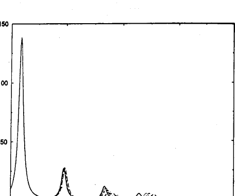
Figure 2: Spectral function for a Heisenberg chain with $N=24$ and $q=\pi$. Full line: exact result [127]. The rest are calculated using DMRG with $m=100$ (long-dashed line), $m=150$ (dashed line) and $m=200$ (dotted line).

In Fig. 3 we show the spectrum for two systems lengths and $q=\pi$ and $q=\pi/2$ keeping $m=200$ states and periodic boundary conditions. For this case it was enough to take 3 target states, i. e.  $|\psi_{0}\rangle$, $|f_{0}\rangle=S^{z}_{\pi}|\psi_{0}\rangle$ and $|f_{1}\rangle$. Here we have used $\sim 40$ pairs of coefficients $a_{n}$ and $b_{n}$, but we noticed that if we considered only the first ($\sim 10$) coefficients $a_{n}$ and $b_{n}$, the spectrum at low energies remains essentially unchanged. Minor differences arise at $\omega/J\simeq 2$. This is another indication that only the first $|f_{n}\rangle$ are relevant for the low energy dynamical properties for finite systems.

In the inset of Fig. 3 the spectrum for $q=\pi/2$ and $N=28$ is shown. For this case we considered 5 target states i. e.  $|\psi_{0}\rangle$, $|f_{0}\rangle=S^{z}_{\pi/2}|\psi_{0}\rangle$, $|f_{n}\rangle\;n=1,3$ and $m=200$. Here, and for all the cases considered, we have verified that the results are very weakly dependent on the weights $p_{l}$ of the target states (see Eq.(2)) as long as the appropriate target states are chosen. For lengths where this value of $q$ is not defined we took the nearest value.

Figure 3: Spectral densities for $q=\pi$, $N=28$ (continuous line) and $N=40$ (dotted line). Inset: Spectral density for $q=\pi/2$ for $N=28$ ($\eta=0.05$).

Even though we are including states with a given momentum as target states, due to the particular real-space construction of the reduced Hilbert space, this translational symmetry is not fulfilled and the momentum is not fixed. To check how the reduction on the Hilbert space influences the momentum $q$ of the target state $|f_{0}\rangle=S^{z}_{q}|\psi_{0}\rangle$, we calculated the expectation values $\langle\psi_{0}|S_{-q^{\prime}}^{z}S_{q}^{z}|\psi_{0}\rangle$ for all $q^{\prime}$. If the momenta of the states were well defined, this value is proportional to $\delta_{q-q^{\prime}}$ if $q\neq 0$. For $q=0$, $\sum_{r}S^{z}_{r}=0$.

The momentum distribution for $q=\pi$ is shown in Fig. 4 in a semilogarithmic scale where the $y$-axis has been shifted by .003 so as to have well-defined logarithms. We can see here that the momentum is better defined, even for much larger systems, but, as expected, more weight on other $q^{\prime}$ values arises for larger $N$.

Figure 4: Momentum weights of a target state with $q=\pi$ for $N=28$ (circles), $N=44$ (squares), $N=60$ (diamonds) and $N=72$ (triangles). The dotted lines are a guide to the eye.

As a check of the approximation we calculated the sum rule

$$\frac{1}{4\pi^{2}}\int_{0}^{\infty}d\omega\int_{q=0}^{2\pi}S^{zz}(q,\omega)\equiv\langle\psi_{0}|(S_{r=0}^{z})^{2}|\psi_{0}\rangle=\frac{1}{4}$$ (12)

for $N=28$, 5 target states and $m=200$. We obtain a relative error of 0.86%.

Recently, important improvements to this method have been published [128]: By considering the finite system method in open chains, Kühner and White obtained a higher precision in dynamical responses of spin chains. In order to define a momentum in an open chain and to avoid end effects, they introduce a filter function with weight centered in the middle of the chain and zero at the boundaries.

In this section we presented a method of calculating dynamical responses with DMRG. Although the basis truncation is big, this method keeps only the most relevant states and, for example, even by considering a $0.1\%$ of the total Hilbert space (for $N=28$ only $\sim$ 40000 states are kept) a reasonable description of the low energy excitations is obtained. We show that it is also possible to obtain states with well defined momenta if the appropriate target states are used.

5.1.1 Correction vector technique

Introduced in Ref. [129] in the DMRG context and improved in Ref. [128], this method focuses on a particular energy or energy window, allowing a more precise description in that range and the possibility of calculating spectra for higher energies. Instead of using the tridiagonalization of the Hamiltonian, but in a similar spirit regarding the important target states to be kept, the spectrum can be calculated for a given $z=w+i\eta$ by using a correction vector (related to the operator $A$ that can depend on momentum $q$).

Following (6), the (complex) correction vector $|x(z)\rangle$ can be defined as:

$$|x(z)\rangle=\frac{1}{z-H}A|\psi_{0}\rangle$$ (13)

so the Green’s function can be calculated as

$$G(z)=\langle\psi_{0}|A^{\dagger}|x(z)\rangle$$ (14)

Separating the correction vector in real and imaginary parts $|x(z)\rangle=|x^{r}(z)\rangle+i|x^{i}(z)\rangle$ we obtain

$$((H-w)^{2}+\eta^{2})|x^{i}(z)\rangle=-\eta A|\psi_{0}\rangle$$ (15)

and

$$|x^{r}(z)\rangle=\frac{1}{\eta}(w-H)|x^{i}(z)\rangle$$ (16)

The former equation is solved using the conjugate gradient method.

In order to keep the information of the excitations at this particular energy the following states are targeted in the DMRG iterations: The ground state $|\psi_{0}\rangle$, the first Lanczos vector $A|\psi_{0}\rangle$ and the correction vector $|x(z)\rangle$. Even though only a certain energy is focused on, DMRG gives the correct excitations for an energy range surrounding this particular point so that by running several times for nearby frequencies, an approximate spectrum can be obtained for a wider region [128].

5.2 Moment expansion

This method[130] relies on a moment expansion of the dynamical correlations using sum rules that depend only on static correlation functions which can be calculated with DMRG. With these moments, the Green’s functions can be calculated using the maximum entropy method.

The first step is the calculation of sum rules. As an example, and following [130], the spin-spin correlation function $S^{z}(q,w)$ of the Heisenberg model is calculated where the operator $A$ of Eq. (4) is $S^{z}(q)=N^{-1/2}\sum S^{z}(l)\exp(iql)$ and the sum rules are[131]:

$$m_{1}(q) = \int_{0}^{\infty}\frac{dw}{\pi}\frac{S^{z}(q,w)}{w}=\frac{1}{2}\chi(q,w=0)$$

$$m_{2}(q) = \int_{0}^{\infty}\frac{dw}{\pi}w\frac{S^{z}(q,w)}{w}=\frac{1}{2}S^{z}(q,t=0)$$

$$m_{3}(q) = \int_{0}^{\infty}\frac{dw}{\pi}w^{2}\frac{S^{z}(q,w)}{w}=-\frac{1}{2}\langle[[H,S^{z}(q)],S^{z}(-q)]\rangle$$ (17)

$$= 2[1-\cos(q)]\sum_{i}\langle S^{+}_{i}S^{-}_{i+1}+S^{-}_{i}S^{+}_{i+1}\rangle$$

where $\chi(q,w=0)$ is the static susceptibility. These sum rules can be easily generalized to higher moments:

$$m_{l}(q) = \int_{0}^{\infty}\frac{dw}{\pi}w^{l-1}\frac{S^{z}(q,w)}{w}$$ (18)

$$= -\frac{1}{2}\langle[[H,...,[H,S^{z}(q)]...],S^{z}(-q)]\rangle$$

for $l$ odd. A similar expression is obtained for $l$ even, where the outer square bracket is replaced by an anticommutator and the total sign is changed. Here $H$ appears in the commutator $l-2$ times.

Apart from the first moment which is given by the static susceptibility, all the other moments can be expressed as equal time correlations (using a symbolic manipulator). The static susceptibility $\chi$ is calculated by applying a small field $h_{q}\sum_{i}n_{i}\cos(qi)$ and calculating the density response $\langle n_{q}\rangle=1/N\sum_{i}\langle n_{q}\rangle\cos(qi)$ with DMRG. Then $\chi=\langle n_{q}\rangle/h_{q}$ for $h_{q}\to 0$. These moments are calculated for several chain lengths and extrapolated to the infinite system. Once the moments are calculated, the final spectra is constructed via the Maximum Entropy method (ME), which has become a standard way to extract maximum information from incomplete data (for details see Ref. [130] and references therein). Reasonable spectra are obtained for the XY and isotropic models, although information about the exact position of the gaps has to be included. Otherwise, the spectra are only qualitatively correct.

This method requires the calculation of a large amount of moments in order to get good results: The more information given to the ME equations, the better the result.

5.3 Finite temperature dynamics

In order to include temperature in the calculation of dynamical quantities, the Transfer Matrix RG described above (TMRG[88, 90, 91]) was extended to obtain imaginary time correlation functions[132, 133, 134]. After Fourier transformation in the imaginary time axis, analytic continuation from imaginary to real frequencies is done using maximum entropy (ME). The combination of the TMRG and ME is free from statistical errors and the negative sign problem of Monte Carlo methods. Since we are dealing with the transfer matrix, the thermodynamic limit can be discussed directly without extrapolations. However, in the present scheme, only local quantities can be calculated.

A systematic investigation of local spectral functions is done in Ref. [134] for the anisotropic Heisenberg antiferromagnetic chain. They obtain good qualitative results especially for high temperatures but a quantitative description of peaks and gaps are beyond the method, due to the severe intrinsic limitation of the analytic continuation. This method was also applied with great success to the 1D Kondo insulator[133]. The temperature dependence of the local density of states and local dynamic spin and charge correlation functions was calculated.

6 Conclusions

We have presented here a very brief description of the Density Matrix Renormalization Group technique, its applications and extensions. The aim of this article is to give the unexperienced reader an idea of the possibilities and scope of this powerful, though relatively simple, method. The experienced reader can find here an extensive (however incomplete) list of references covering most applications to date using DMRG, in a great variety of fields such as Condensed Matter, Statistical Mechanics and High Energy Physics.

References

- [1] S. White, Phys. Rev. Lett. 69, 2863 (1992)
- [2] Density Matrix Renormalization, edited by I. Peschel, X. Wang, M. Kaulke and K. Hallberg (Series: Lecture Notes in Physics, Springer, Berlin, 1999)
- [3] S. White, Phys. Rev. B 48, 10345 (1993)
- [4] J. Bray and S. Chui, Phys. Rev. B 19, 4876 (1979)
- [5] C. Pan and X. Chen, Phys. Rev. B 36, 8600 (1987); M. Kovarik, Phys. Rev. B 41, 6889 (1990)
- [6] T. Xiang and G. Gehring, Phys. Rev. B 48, 303 (1993)
- [7] K. Wilson, Rev. Mod. Phys. 47, 773 (1975)
- [8] S. White and R. Noack, Phys. Rev. Lett. 68, 3487, (1992); R. Noack and S. White, Phys. Rev. B 47, 9243 (1993)
- [9] R. Noack and S. White in Ref. [2], Chap. 2(I)
- [10] M. Martín-Delgado, G. Sierra and R. Noack, J. Phys. A: Math. Gen. 32, 6079 (1999)
- [11] R.P. Feynman, Statistical Mechanics: A Set of Lectures, (Benjamin, Reading, MA, 1972)
- [12] See E. Dagotto, Rev. Mod. Phys. 66, 763 (1994)
- [13] E. R. Davidson, J. Comput. Phys. 17, 87 (1975); E.R. Davidson, Computers in Physics 7, No. 5, 519 (1993).
- [14] S. White, Phys. Rev. Lett. 77, 3633 (1996)
- [15] T. Nishino and K. Okunishi, Phys. Soc. Jpn. 64, 4084 (1995); U. Schollwöck, Phys. Rev. B 58, 8194 (1998) and Phys. Rev. B 59, 3917 (1999) (Erratum).
- [16] Ö. Legeza and G. Fáth, Phys. Rev. B 53, 14349 (1996); M-B Lepetit and G. Pastor, Phys. Rev. B 58, 12691 (1998)
- [17] S. Östlund and S. Rommer, Phys. Rev. Lett. 75, 3537 (1995); Phys. Rev. B 55, 2164 (1997); M. Andersson, M. Boman and S. Östlund, Phys. Rev. B 59, 10493 (1999); H. Takasaki, T. Hikihara and T. Nishino, J. Phys. Soc. Jpn. 68, 1537 (1999); K. Okunishi, Y. Hieida and Y.Akutsu, Phys. Rev. E 59, R6227 (1999)
- [18] M. A. Martín-Delgado and G. Sierra, Int. J. Mod. Phys. A, 11, 3145 (1996)
- [19] G. Sierra and M. A. Martín-Delgado, in ”The Exact Renormalization Group ” by a Krasnitz, R Potting, P S De S, Y A Kubyshin, P. S. de Sa (Eds) World Scientific Pub Co; ISBN: 9810239394, (1999), (cond-mat/9811170)
- [20] I. Peschel, M. Kaulke and Ö. Legeza, Annalen der Physik 8, 153 (1999),(cond-mat/9810174)
- [21] Steven White and David Huse, Phys. Rev. B 48, 3844 (1993)
- [22] E. S. Sørensen and I. Affleck, Phys. Rev. B 49, 13235 (1994)
- [23] E. S. Sørensen and I. Affleck, Phys. Rev. B 49, 15771 (1994); E. Polizzi, F. Mila and E. Sørensen, Phys. Rev. B 58, 2407 (1998)
- [24] C. Batista, K. Hallberg and A. Aligia, Phys. Rev. B 58, 9248 (1998); Phys. Rev. B 60, 12553 (1999)
- [25] M. Laukamp et al., Phys. Rev. B 5, 10755 (1998)
- [26] Y. Nishiyama, K. Totsuka, N. Hatano and M. Suzuki, J. Phys. Soc. Jpn 64, 414 (1995)
- [27] S. Qin, T. Ng and Z-B Su, Phys. Rev. B 52, 12844 (1995)
- [28] U. Schollwöck and T. Jolicoeur, Europhys. Lett. 30, 493 (1995)
- [29] X. Wang, S. Qin and Lu Yu, cond-mat/9903035
- [30] W. Tatsuaki, cond-mat/9909003
- [31] S. Qin, X. Wang and Lu Yu, Phys. Rev. B 56, R14251 (1997)
- [32] K. Hallberg, P. Horsch and G. Martínez, Phys. Rev. B, 52, R719 (1995)
- [33] T. Hikihara and A. Furusaki, Phys. Rev. B 58, R583 (1998)
- [34] K. Hallberg, X. Wang, P. Horsch and A. Moreo, Phys. Rev. Lett. 76, 4955 (1996)
- [35] A. Moreo, Phys. Rev. B 35, 8562 (1987); T. Ziman and H. Schulz, Phys. Rev. Lett 59, 140 (1987)
- [36] Y. Yamashita, N. Shibata and K. Ueda, Phys. Rev. B 58, 9114 (1998); cond-mat/9908237
- [37] A. Onufriev and B. Marston, Phys. Rev. B 59, 12573 (1999)
- [38] R. J. Bursill, T. Xiang and G. A. Gehring, J. Phys. A 28 2109 (1994)
- [39] R. J. Bursill, G. A. Gehring, D. J. J. Farnell, J. B. Parkinson, Tao Xiang and Chen Zeng, J. Phys. C 7 8605 (1995)
- [40] U. Schollwöck, Th. Jolicoeur and T. Garel, Phys. Rev. B 53 3304 (1996)
- [41] R. Chitra, S. Pati, H. R. Krishnamurthy, D. Sen and S. Ramasesha, Phys. Rev. B 52 6581 (1995); S. Pati, R. Chitra, D. Sen, H. R. Krishnamurthy and S. Ramasesha, Europhys. Lett. 33 707 (1996); J. Malek, S. Drechsler, G. Paasch and K. Hallberg, Phys. Rev. B 56, R8467 (1997); E. Sørensen et al in Ref.[2], Chap.1.2 (Part II) and references therein; D. Augier, E. Sørensen, J. Riera and D. Poilblanc, Phys. Rev. B 60, 1075 (1999)
- [42] Y. Kato and A. Tanaka, J. Phys. Soc. Jap. 63 1277 (1994)
- [43] S. R. White and I. Affleck, Phys. Rev. B 54, 9862 (1996)
- [44] G. Bouzerar, A. Kampf and G. Japaridze, Phys. Rev. B 58, 3117 (1998); G. Bouzerar, A. Kampf and F. Schönfeld, cond-mat/9701176, unpublished; M.-B. Lepetit and G. Pastor, Phys. Rev. B 56, 4447 (1997)
- [45] M. Kaburagi, H. Kawamura and T. Hikihara, cond-mat/9902002 (to appear in J. Phys. Soc. Jpn.)
- [46] S. Pati, S. Ramasesha and D. Sen, Phys. Rev. B 55, 8894 (1996); J. Phys. Cond. Matt. 9, 8707 (1997); T. Tonegawa et al, J. Mag. 177-181, 647 (1998), (cond-mat/9712298)
- [47] M. Azzouz, L. Chen and S. Moukouri, Phys. Rev. B 50 6223 (1994); S. R. White, R. M. Noack and D. J. Scalapino, Phys. Rev. Lett. 73 886 (1994); K. Hida, J. Phys. Soc. Jap. 64 4896 (1995); T. Narushima, T. Nakamura and S. Takada, J. Phys. Soc. Jap. 64 4322 (1995); U. Schollwöck and D. Ko, Phys. Rev. B 53 240 (1996); G. Sierra, M. A. Martín-Delgado, S. White and J. Dukelsky, Phys. Rev. B 59, 7973 (1999); S. White, Phys. Rev. B 53, 52 (1996)
- [48] K. Tandon et al, Phys. Rev. B 59, 396 (1999); R. Citro, E. Orignac, N. Andrei, C. Itoi and S. Qin, cond-mat/9904371
- [49] L. Chen and S. Moukouri, Phys. Rev. B 53 1866 (1996); S. J. Qin, S. D. Liang, Z. B. Su and L. Yu, Phys. Rev. B 52 R5475 (1995); R. Noack in Ref.[2], Chap.1.3 (Part II); S. Daul and R. Noack, cond-mat/9907256; M. Vojta, R. Hetzel and R. Noack, cond-mat/9906101
- [50] R. M. Noack, S. R. White and D. J. Scalapino, Phys. Rev. Lett. 73 882 (1994); S. R. White, R. M. Noack and D. J. Scalapino, J. Low Temp. Phys. 99 593 (1995); R. M. Noack, S. R. White and D. J. Scalapino, Europhys. Lett. 30 163 (1995); C. A. Hayward, D. Poilblanc, R. M. Noack, D. J. Scalapino and W. Hanke, Phys. Rev. Lett. 75 926 (1995); S. White and D. Scalapino, Phys. Rev. Lett. 81, 3227 (1998); E. Jeckelmann, D. Scalapino and S. White, Phys. Rev. B 58, 9492 (1998)
- [51] S. Liang and H. Pang, Europhys. Lett. 32, 173 (1995)
- [52] S. White and D. Scalapino, Phys. Rev. B 55, 14701 (1997)
- [53] S. White and D. Scalapino, Phys. Rev. B 55, 6504 (1997)
- [54] S. White and D. Scalapino, Phys. Rev. B 57, 3031 (1998)
- [55] S. White and D. Scalapino, Phys. Rev. Lett. 80, 1272 (1998)
- [56] T. A. Costi, P. Schmitteckert, J. Kroha and P. Wölfle, Phys. Rev. Lett. 73 1275 (1994); S. Eggert and I. Affleck, Phys. Rev. Lett. 75 934 (1995); E. S. Sørensen and I. Affleck, Phys. Rev. B 51 16115 (1995); X. Q. Wang and S. Mallwitz, Phys. Rev. B 53 R492 (1996); W. Wang, S. J. Qin, Z. Y. Lu, L. Yu and Z. B. Su, Phys. Rev. B 53 40 (1996); C. C. Yu and M. Guerrero, Phys. Rev. B 54, 15917 (1996); A. Furusaki and T. Hikihara, Phys. Rev. B 58, 5529 (1998)
- [57] K. Hallberg and R. Egger, Phys. Rev. B 55, 8646 (1997)
- [58] C. C. Yu and S. R. White, Phys. Rev. Lett. 71 3866 (1993); C. C. Yu and S. R. White, Physica B 199 454 (1994)
- [59] S. Moukouri and L. G. Caron, Phys. Rev. B 52 15723 (1995); N. Shibata, T. Nishino, K. Ueda and C. Ishii, Phys. Rev. B 53 R8828 (1996); M. Guerrero and R. M. Noack, Phys. Rev. B 53 3707 (1996)
- [60] H. Otsuka and T. Nishino, Phys. Rev. B 52 15066 (1995); S. Moukouri, L. G. Caron, C. Bourbonnais and L. Hubert, Phys. Rev. B 51 15920 (1995)
- [61] S. Watanabe, Y. Kuramoto, T. Nishino and N. Shibata, J. Phys. Soc. Jpn 68, 159 (1999)
- [62] S. Moukouri, L. Chen and L. G. Caron, Phys. Rev. B 53 R488 (1996)
- [63] J. Riera, K. Hallberg and E. Dagotto, Phys. Rev. Lett. 79, 713 (1997); E. Dagotto et al., Phys. Rev. B 58, 6414 (1998)
- [64] S. Ramasesha et al, Phys. Rev. B 54, 7598 (1996); Synth. Metals 85, 1019 (1997)
- [65] E. S. Sørensen and I. Affleck, Phys. Rev. B 51 16115 (1995)
- [66] I. McCulloch, M. Gulacsi, S. Caprara, A. Juozapavicius and A. Rosengren, cond-mat/9908414
- [67] G. Sierra and T. Nishino, Nucl. Phys. B 495, 505 (1997) (cond-mat/9610221)
- [68] T. Xiang, Phys. Rev. B 53, R10445 (1996)
- [69] M.S.L. du Croo de Jongh and J.M.J. van Leeuwen, Phys. Rev. B 57, 8494 (1998)
- [70] M-B. Lepetit, M. Cousy and G. Pastor, accepted in Eur. Phys. J B, (1999); H. Otsuka, Phys. Rev. B 53, 14004 (1996)
- [71] J. Dukelsky and G. Dussel, Phys. Rev. B 59, R3005 (1999) and references therein.
- [72] J. Dukelsky and G. Sierra, Phys. Rev. Lett. 83, 172 (1999)
- [73] M. A. Martín-Delgado and G. Sierra, Phys. Rev. Lett. 83, 1514 (1999)
- [74] S. Glazek and K. Wilson, Phys. Rev. D 48, 5863 (1993); 49, 4214 (1994)
- [75] T. Eller, H.-C. Pauli and S. Brodsky, Phys. Rev. D 35, 1493 (1987)
- [76] T. Nishino, J. Phys. Soc. Jpn. 64, 3598 (1995); see also T. Nishino in Ref. [2], Chap. 5(I); T. Nishino and K. Okunishi in Strongly Correlated Magnetic and Superconducting Systems, Ed. G. Sierra and M. A. Martín-Delgado (Springer, Berlin, 1997)
- [77] H. Trotter, Proc. Am. Math. Soc. 10, 545 (1959); M. Suzuki, Prog. Theor. Phys. 56, 1454 (1976); R. Feynman and A. Hibbs Quantum Mechanics and Path Integrals (McGraw-Hill, 1965)
- [78] R. Baxter, J. Math. Phys. 9, 650 (1968); J. Stat Phys. 19, 461 (1978)
- [79] T. Nishino and K. Okunishi, J. Phys. Soc. Jpn. 65,891 (1996); ibid. 66, 3040 (1997); T. Nishino, K. Okunishi and M. Kikuchi, Phys. Lett. A 213, 69 (1996)
- [80] T. Nishino and K. Okunishi, J. Phys. Soc. Jpn. 67, 3066 (1998)
- [81] E. Carlon and A. Drzewiński, Phys. Rev. Lett. 79, 1591 (1997); Phys. Rev. E 57, 2626 (1998); E. Carlon, A. Drzewiński and J. Rogiers, Phys. Rev. B 58, 5070 (1998); A. Drzewiński, A. Ciach and A. Maciolek, Eur. Phys. J. B 5, 825 (1998); Phys. Rev. E 60, 2887 (1999)
- [82] E. Carlon and F. Iglói, Phys. Rev. B 57, 7877 (1998); Phys. Rev. B 59, 3783 (1999)
- [83] J. Kondev and J. Marston, Nucl. Phys. B 497, 639 (1997); T. Senthil, B. Marston and M. Fisher, Phys. Rev. B 60, 4245 (1999); J. Marston and S. Tsai, Phys. Rev. Lett. 82, 4906 (1999); cond-mat/9908180
- [84] M. Kaulke and I. Peschel, Eur. Phys. J. B 5, 727 (1998)
- [85] Y. Hieida, J. Phys. Soc. Jpn. 67, 369 (1998)
- [86] I. Peschel and M. Kaulke, in Ref. [2], Chap. 3.1(II)
- [87] E. Carlon, M. Henkel and U. Schollwöck, cond-mat/9902041
- [88] R. Bursill, T. Xiang and G. Gehring, J. Phys. C 8, L583 (1996)
- [89] H. Trotter, Proc. Am. Math. Soc. 10, 545 (1959); M. Suzuki, Prog. Theor. Phys. 56, 1454 (1976)
- [90] X. Wang and T. Xiang, Phys. Rev. B 56, 5061 (1997)
- [91] N. Shibata, J. Phys. Soc. Jpn. 66, 2221 (1997)
- [92] T. Xiang, Phys. Rev. B 58, 9142 (1998)
- [93] N. Shibata, B. Ammon, T. Troyer, M. Sigrist and K. Ueda, J. Phys. Soc. Jpn. 67, 1086 (1998)
- [94] K. Maisinger, U. Schollwöck, S. Brehmer, H.-J. Mikeska and S. Yamamoto, Phys. Rev. B 58, R5908 (1998)
- [95] S. Rommer and S. Eggert, Phys. Rev. B, Phys. Rev. B 59, 6301 (1999)
- [96] K. Maisinger and U. Schollwöck, Phys. Rev. Lett. 81, 445 (1999)
- [97] B. Ammon, M. Troyer, T. Rice and N. Shibata, Phys. Rev. Lett. 82, 3855 (1999); N. Shibata and H. Tsunetsugu, cond-mat/9907416
- [98] A. Klümper, R. Raupach and F. Schönfeld, Phys. Rev. B 59, 3612 (1999)
- [99] S. Moukouri and L. Caron, Phys. Rev. Lett. 77, 4640 (1996).
- [100] S. Moukouri and L. Caron, see Ref.[2], Chap. 4.5(II)
- [101] W. Zhang, J. Igarashi and P. Fulde, J. Phys. Soc. Jpn. 66, 1912 (1997)
- [102] L. Caron and S. Moukouri, Phys. Rev. Lett. 76, 4050 (1996); Phys. Rev. B 56, R8471 (1997).
- [103] E. Jeckelmann and S. White, Phys. Rev. B 57, 6376 (1998)
- [104] R. Noack, S. White and D. Scalapino in Computer Simulations in Condensed Matter Physics VII, edited by D. Landau, K.-K. Mon and H.-B. Schüttler (Springer Verlag, Heidelberg and Berlin, 1994)
- [105] E. Jeckelmann, C. Zhang and S. White in Ref. [2], Chap. 5.1 (II)
- [106] C. Zhang, E. Jeckelmann and S. White, Phys. Rev. Lett. 80, 2661 (1998)
- [107] R. Bursill, Y. McKenzie and C. Hammer, Phys. Rev. Lett. 80, 5607 (1998); 83, 408 (1999); R. Bursill, Phys. Rev. B 60, 1643 (1999)
- [108] R. Pai, R. Pandit, H. Krishnamurthy and S. Ramasesha, Phys. Rev. Lett. 76, 2937 (1996); S. Rapsch, U. Schollwöck and W. Zwerger, cond-mat/9901080
- [109] T. Kühner and H. Monien, Phys. Rev. B 58, R14741 (1998)
- [110] K. Hida, J. Phys. Soc. Jpn. 65, 895 (1996) and 3412 (1996) (errata); J. Phys. Soc. Jpn. 66, 330 (1997); J. Phys. Soc. Jpn. 66, 3237 (1997)
- [111] K. Hida, J. Phys. Soc. Jpn. in press, cond-mat/9907115
- [112] K. Hida, Phys. Rev. Lett. 83, 3297 (1999)
- [113] P. Schmitteckert, T. Schulze, C. Cosima, P. Schwab and U. Eckern, Phys. Rev. Lett. 80, 560 (1998); P. Schmitteckert and U. Eckern, Phys. Rev. B 53, 15397 (1996)
- [114] P. Schmitteckert, R. Jalabert, D. Weinmann and J. L. Pichard, Phys. Rev. Lett. 81, 2308 (1998)
- [115] G. Fano, F. Ortolani and L. Ziosi, J. Chem. Phys. 108, 9246 (1998),(cond-mat/9803071); R. Bursill and W. Barford, Phys. Rev. Lett. 82, 1514 (1999)
- [116] W. Barford and R. Bursill, Chem. Phys. Lett. 268, 535(1997); W. Barford, R. Bursill and M. Lavrentiev, J. Phys: Cond. Matt, 10, 6429 (1998); W. Barford in Ref.[2], Chap.2.3 (Part II) and references therein.
- [117] S. White and R. Martin, J. Chem. Phys. 110, 4127 (1999); see also S. White in [2], Chap. 2.1.
- [118] S. White in Ref. [2], Chap. 2.1.
- [119] C. Bauschlicher and P. Taylor, J. Chem. Phys. 85, 2779 (1986)
- [120] K. Hallberg, Phys. Rev. B 52, 9827 (1995).
- [121] E. R. Gagliano and C. A. Balseiro, Phys. Rev. Lett. 59, 2999 (1987).
- [122] G. Grosso and G. Partori Parravicini, in Memory Function Approaches to Stochastic Problems in Condensed Matter, Adv. in Chemical Physics, 62, 133 (Wiley, N. Y., 1985)
- [123] P. Horsch and W. von der Linden, Z. Phys. B 72 181 (1981)
- [124] J. des Cloiseaux and J. J. Pearson, Phys. Rev. 128, 2131 (1962)
- [125] T. Yamada, Prog. Theor. Phys. Jpn. 41, 880 (1969); L. D. Fadeev and L. A. Takhtajan, Phys. Lett. 85 A, 375 (1981)
- [126] G. Müller, H. Thomas, H. Beck and J. Bonner, Phys. Rev. B 24, 1429 (1981) and references therein.
- [127] S. Haas, J. Riera and E. Dagotto, Phys. Rev. B 48, 3281 (1993)
- [128] T. Kühner and S. White, Phys. Rev. B 60, 335(1999)
- [129] Y. Anusooya, S. Pati and S. Ramasesha, J. Chem. Phys. 106, 1 (1997); S. Ramasesha, K. Tandon, Y. Anusooya and S. Pati, Proc. of SPIE, 3145, 282 (1997); S. Ramasesha, Z. Shuai and J. Brédas, Chem. Phys. Lett. 245, 224 (1995)
- [130] H. B. Pang, H. Akhlaghpour and M. Jarrell, Phys. Rev. B 53 5086 (1996)
- [131] P. Hohenberg and W. Brinkman, Phys. Rev. B 10, 128 (1974)
- [132] X. Wang, K. Hallberg and F. Naef in Ref.[2], Chap.7(I)
- [133] T. Mutou, N. Shibata and K. Ueda, Phys. Rev. Lett 81, 4939 (1998)
- [134] F. Naef, X. Wang, X. Zotos and W. von der Linden, Phys. Rev. B 60, 359 (1999)