Abstract

We explore a nonlinear field model to describe the interplay between the ability of excitons to be Bose-condensed and their interaction with other modes of a crystal. We apply our consideration to the long-living para-excitons in Cu₂O. Taking into account the exciton-phonon interaction and introducing a coherent phonon part of the moving condensate, we derive the dynamic equations for the exciton-phonon condensate. These equations can support localized solutions, and we discuss the conditions for the moving inhomogeneous condensate to appear in the crystal. We calculate the condensate wave function and energy, and a collective excitation spectrum in the semiclassical approximation; the inside-excitations were found to follow the asymptotic behavior of the macroscopic wave function exactly. The stability conditions of the moving condensate are analyzed by use of Landau arguments, and Landau critical parameters appear in the theory. Finally, we apply our model to describe the recently observed interference and strong nonlinear interaction between two coherent exciton - phonon packets in Cu₂O.

PACS numbers: 71.35.+z, 71.35.Lk

1 Introduction

Excitons in semiconductor crystals [1] and nanostructures [2],[3] are a very interesting and challenging object to search for the process of Bose-Einstein condensation (BEC). Nowadays there is a lot of experimental evidence that the optically inactive para-excitons in Cu₂O can form a highly correlated state, or the excitonic Bose Einstein condensate [1],[4],[5]. A moving condensate of para-excitons in a 3D Cu₂O crystal turns out to be spatially inhomogeneous in the direction of motion, and the registered velocities of coherent exciton packets turn out to be always less, but approximately equal to the longitudinal sound speed of the crystal [6].

Analyzing recent experimental [4],[6],[7] and theoretical [8]-[13] studies of BEC of excitons in Cu₂O, we can conclude that there are essentially two different stages of this process. The first stage is the kinetic one, with the characteristic time scale of $10\sim 20$ ns. At this stage, a condensate of long-living para-excitons begins to be formed from a quasi-equilibrium degenerate state of excitons ($\mu\neq 0$, $T_{\rm eff}>T_{\rm latt}$) when the concentration and the effective temperature of excitons in a cloud meet the conditions of Bose-Einstein Condensation [1]. Note that we do not discuss here the behavior of ortho-excitons (with the lifetime $\tau_{\rm ortho}\simeq 30$ ns) and their influence on the para-exciton condensation process. For more details about the ortho-excitons in Cu₂O, ortho-para-exciton conversion, etc. see [4],[5], [14], [15].

The most intriguing feature of the kinetic stage is that formation of the para-exciton condensate and the process of momentum transfer to the para-exciton cloud are happening simultaneously. If the diameter of an excitation spot on the crystal surface is large enough,  $S_{\rm spot}\simeq S_{\rm surf}$,   and the energy of a laser beam satisfies $\epsilon_{\rm phot}\gg E_{\rm gap}$, nonequilibrium acoustic phonons may play the key role in the process of momentum transfer. As a result, the mode with macroscopical occupancy of the excitons appears to be with $\langle{\bf k}\rangle\neq 0,$ where $\hbar\langle k_{x}\rangle=m_{\rm x}\,v$ and $v$ is the packet velocity.

Indeed, the theoretical results obtained in the framework of the “phonon wind” model [10],[16] and the experimental observations [4],[5],[6] are the strong arguments in favor of this idea. To the authors’ knowledge, there are no realistic theoretical models of the kinetic stage of para-exciton condensate formation where quantum degeneracy of the appearing exciton state and possible coherence of nonequilibrium phonons pushing the excitons would be taken into account. Indeed, the condensate formation and many other processes involving it are essentially nonliner ones. Therefore, the condensate, or, better, the macroscopically occupied mode, can be different from $n({\bf k}=0)\gg 1$, and the language of the states in ${\bf k}$-space and their occupation numbers $n({\bf k})$ may be not relevant to the problem, see [17].

In this study, we will not explore the stage of condensate formation. Instead, we investigate the second, quasi-equilibrium stage, in which the condensate has already been formed and it moves through a crystal with some constant velocity and characteristic shape of the density profile. In theory, the time scale of this “transport” stage, $\Delta t_{\rm tr}$, could be determined by the para-exciton lifetime ($\tau_{\rm para}\simeq 13\,\,\mu$s [1]). In practice, it is determined by the characteristic size $\ell$ of a high-quality single crystal available for experiments:

$$\Delta t_{\rm tr}\simeq\ell/c_{l}\simeq 0.5-2\,\mu{\rm s}\ll\tau_{\rm para},$$

where $c_{l}$ is the longitudinal sound velocity.

We assume that at the “transport” stage, the temperature of the moving packet (condensed $+$ noncondensed particles) is approximately equal to the lattice temperature,

$$T_{\rm eff}=T_{\rm latt}<T_{c}.$$

Then we can consider the simplest case of $T=0$ and disregard the influence of all sorts of nonequilibrium phonons (which appear at the stages of exciton formation, thermalization [10] ) on the formed moving condensate.

Any theory of the exciton BEC in Cu₂O has to point out some physical mechanism(s) by means of which the key experimental facts can be explained. (For example, the condensate moves without friction within a narrow interval of velocities localized near $c_{l}$, and the shape of the stable macroscopic wave function of excitons resembles soliton profiles [7].) Here we explore a simple model of the ballistic exciton-phonon condensate. In this case, the general structure of the Hamiltonian of the moving exciton packet and the lattice phonons is the following:

$$\hat{H}=H_{\rm ex}(\hat{\psi}^{{\dagger}},\hat{\psi})-{\bf v}{\bf P}_{\rm ex}(\hat{\psi}^{{\dagger}},\hat{\psi})+H_{\rm ph}(\hat{{\bf u}},\hat{\pi})-{\bf v}{\bf P}_{\rm ph}(\hat{{\bf u}},\hat{\pi})+H_{\rm int}(\hat{\psi}^{{\dagger}}\hat{\psi},\,\partial_{j}\hat{u}_{k}).$$ (1)

Here $\hat{\psi}$ is the Bose-field operator describing the excitons, $\hat{\bf u}$ is the field operator of lattice displacements, $\hat{\pi}$ is the momentum density operator canonically conjugate to $\hat{\bf u}$, and ${\bf P}$ is the momentum operator. Note that the Hamiltonian (1) is written in the reference frame moving with the exciton packet, i.e. ${\bf x}\rightarrow{\bf x}-{\bf v}t$ and ${\bf v}={\rm const}$ is the ballistic velocity of the packet.

2 3D Model of Moving Exciton-Phonon Condensate

To derive the equations of motion of the field operators (and generalize these equations to the case of $T\neq 0$), it is more convenient to start from the Lagrangian. In the proposed model, the Lagrangian density has the following form in the co-moving frame

$${\cal L}={{i\hbar}\over{2}}(\hat{\psi}^{{\dagger}}\,\partial_{t}\hat{\psi}-\partial_{t}\hat{\psi}^{{\dagger}}\,\hat{\psi})+\,v{{i\hbar}\over{2}}(\partial_{x}\hat{\psi}^{{\dagger}}\,\hat{\psi}-\hat{\psi}^{{\dagger}}\partial_{x}\hat{\psi})-$$

$$-\tilde{E}_{g}\hat{\psi}^{{\dagger}}\hat{\psi}-{{\hbar^{2}}\over{2m}}\nabla\hat{\psi}^{{\dagger}}\nabla\hat{\psi}-{{\nu_{0}}\over{2}}\bigl{(}\psi^{{\dagger}}({\bf x},t)\bigr{)}^{2}\bigl{(}\psi({\bf x},t)\bigr{)}^{2}-{{\nu_{1}}\over{3}}\bigl{(}\psi^{{\dagger}}({\bf x},t)\bigr{)}^{3}\bigl{(}\psi({\bf x},t)\bigr{)}^{3}+$$

$$+{{\rho}\over{2}}(\partial_{t}\hat{\bf u})^{2}-{{\rho c_{l}^{2}}\over{2}}(\,\partial_{j}\hat{u}_{s}\,)^{2}-{{\rho c_{l}^{2}}\over{2}}\,\kappa_{3}\,(\partial_{j}\hat{u}_{s}\,)^{3}-\frac{\rho v}{2}\,(\partial_{t}\hat{\bf u}\,\partial_{x}\hat{\bf u}+\partial_{x}\hat{\bf u}\,\partial_{t}\hat{\bf u}\,)+{{\rho v^{2}}\over{2}}(\partial_{x}\hat{\bf u})^{2}-$$

$$-\sigma_{0}\hat{\psi}^{{\dagger}}({\bf x},t)\hat{\psi}({\bf x},t)\nabla\hat{\bf u}({\bf x},t),$$ (2)

where $m$ is the exciton “bare”mass ($m=m_{e}+m_{h}\simeq 3m_{e}$ for $1$s excitons in Cu₂O),  $\nu_{0}$ is the exciton-exciton interaction constant ($\nu_{0}>0$ corresponds to the repulsive interaction between para-excitons in Cu₂O [18]), $\rho$ is the crystal density, $\sigma_{0}$ is the exciton-longitudinal phonon coupling constant, and ${\bf v}=(v,0,0)$. The energy of a free exciton is $\tilde{E}_{g}+\hbar^{2}{\bf k}^{2}/2m$. Although the validity of the condition $n\,\tilde{a}_{\rm B}^{3}\ll 1$ ($\tilde{a}_{\rm B}$ is the exciton Bohr radius) makes it possible to disregard all the multiple-particle interactions with more than two participating particles in $\hat{H}_{\rm ex}$ [19], we include the hard-core repulsion term originated from the three-particle interaction in $\cal L$, i.e. $\nu_{1}\neq 0$  and

$$0<\nu_{1}/\tilde{a}_{\rm B}^{6}\ll\nu_{0}/\tilde{a}_{\rm B}^{3}\simeq{\rm const}\,{\rm Ry}^{*}.$$

(For 3D case, one has to take  ${\rm const}\simeq 10$ because  $\nu_{0}=4\pi\,(\hbar^{2}/m)\,a_{\rm sc}$ and $a_{\rm sc}\simeq(1\sim 3)\,\tilde{a}_{\rm B}$; see the discussion in [20].)

Moreover, in the Lagrangian of the displacement field, we include the first nonlinear term  $\propto\kappa_{3}\,(\partial u)^{3}$. (The dimensionless parameter $\kappa_{3}$ originates from Taylor’s expansion of an interparticle potential  $U(|r_{i}-r_{j}|)$   of the medium atoms.) Assuming that a dilute excitonic packet moves in a weekly nonlinear medium, we will not take into account more higher nonlinear terms in (2).

For simplicity’s sake, we take all the interaction terms in ${\cal L}$ in the local form and disregard the interaction between the excitons and transverse phonons of the crystal. Note that the ballistic velocity $v$ is one of the parameters of the theory, and we will not take into account the excitonic normal component and velocity, i.e. $v=v_{s}\sim\nabla\varphi_{\rm c}$,   $(T=0)$. This means that we choose the spatial part of the coherent phase of the packet, $\varphi_{\rm c}({\rm x})$, to be in the simplest form,

$$\exp\bigl{(}i\varphi_{\rm c}({\rm x})\bigr{)}=\exp\bigl{(}i(\varphi+k_{0}x)\bigr{)},\,\,\,\,\,\varphi={\rm const},\,\,\,\,\,\hbar k_{0}=mv.$$ (3)

The equations of motion can be easily derived by the standard variational method from the following condition:

$$\delta S=\delta\!\int dt\,d{\bf x}\,{\cal L}\bigl{(}\hat{\psi}^{{\dagger}}({\bf x},t),\,\hat{\psi}({\bf x},t),\,\hat{\bf u}({\bf x},t)\bigr{)}=0.$$

Indeed, after transforming the Bose-fields $\hat{\psi}^{{\dagger}}$ and $\hat{\psi}$ by

$$\hat{\psi}({\bf x},t)\rightarrow\exp(-i\tilde{E}_{g}t/\hbar)\exp(imvx/\hbar)\hat{\psi}({\bf x},t),$$

we can write these equations as follows:

$$(i\hbar\partial_{t}+mv^{2}/2)\hat{\psi}({\bf x},t)=$$

$$=\Bigr{(}-{{\hbar^{2}}\over{2m}}\Delta+\nu_{0}\hat{\psi}^{{\dagger}}\hat{\psi}({\bf x},t)+\nu_{1}\hat{\psi}^{{\dagger}\,2}\hat{\psi}^{2}({\bf x},t)\,\Bigl{)}\hat{\psi}({\bf x},t)+\sigma_{0}\nabla\hat{\bf u}({\bf x},t)\,\hat{\psi}({\bf x},t),$$ (4)

$$\bigl{(}\partial_{t}^{2}-c_{l}^{2}\Delta-v(\partial_{t}\partial_{x}+\partial_{x}\partial_{t})+v^{2}\partial_{x}^{2}\bigr{)}\hat{u}_{s}({\bf x},t)-c_{l}^{2}\sum_{j}\!2\kappa_{3}\,\partial_{j}^{2}\hat{u}_{s}\,\partial_{j}\hat{u}_{s}({\bf x},t)=\rho^{-1}\sigma_{0}\partial_{s}\bigl{(}\hat{\psi}^{{\dagger}}\hat{\psi}({\bf x},t)\bigr{)}.$$ (5)

We assume that the condensate of excitons exists. This means that the following representation of the exciton Bose-field holds: $\hat{\psi}=\psi_{0}+\delta\hat{\psi}$. Here $\psi_{0}\neq 0$ is the classical part of the field operator $\hat{\psi}$ or, in other words, the condensate wave function, and $\delta\hat{\psi}$ is the fluctuational part of $\hat{\psi}$, which describes out-of-condensate particles.

One of the important objects in the theory of BEC is the correlation functions of Bose-fields. The standard way to calculate them in this model (the excitonic function $\langle\psi({\bf x},t)\psi^{{\dagger}}({\bf x}^{\prime},t^{\prime})\rangle$, for example,) can be based on the effective action or the effective Hamiltonian approaches [21]. Indeed, one can, first, integrate over the phonon variables ${\bf u}$, get the expression for $S_{\rm eff}(\psi,\psi^{{\dagger}})$ and, second, use $S_{\rm eff}$ (or $\hat{H}_{\rm eff}$) to derive the equations of motion for $\psi_{0}$, $\delta\hat{\psi}$, correlation functions, etc..

In this work we do not follow that way; instead, we treat excitons and phonons equally [11],[22],[23]. This means that the displacement field $\hat{\bf u}$ can have a nontrivial coherent part too, i.e. $\hat{\bf u}={\bf u}_{0}+\delta\hat{\bf u}$ and ${\bf u}_{0}\neq 0$, and the actual moving condensate can be an exciton-phonon one, i.e. $\psi_{0}({\bf x},t)\cdot{\bf u}_{0}({\bf x},t)$. Then the equation of motion for the classical parts of the fields $\hat{\psi}$ and $\hat{\bf u}$ can be derived by use of the variational method from ${\cal L}={\cal L}(\psi,\psi^{*},{\bf u})$, in which all the fields can be considered as the classical ones. Eventually we have

$$(\,i\hbar\partial_{t}+mv^{2}/2\,){\psi}_{0}({\bf x},t)=$$

$$=\Bigr{(}-{{\hbar^{2}}\over{2m}}\Delta+\nu_{0}|{\psi_{0}}|^{2}({\bf x},t)+\nu_{1}|{\psi}_{0}|^{4}({\bf x},t)\,\Bigl{)}{\psi}_{0}({\bf x},t)+\sigma_{0}\nabla{\bf u}_{0}({\bf x},t)\,{\psi}_{0}({\bf x},t)\,,$$ (6)

$$\bigl{(}\partial_{t}^{2}-c_{l}^{2}\Delta-2v\partial_{t}\partial_{x}+v^{2}\partial_{x}^{2}\bigr{)}{u}_{0\,s}({\bf x},t)-c_{l}^{2}\sum_{j}\!2\kappa_{3}\,\partial_{j}^{2}{u}_{0\,s}\,\partial_{j}{u}_{0\,s}({\bf x},t)=\rho^{-1}\sigma_{0}\partial_{s}\bigl{(}|\psi_{0}|^{2}({\bf x},t)\bigr{)}.$$ (7)

Notice that deriving these equations we disregarded the interaction between the classical (condensate) and the fluctuational (noncondensate) parts of the fields. That is certainly a good approximation for $T=0$ and $T\ll T_{c}$ cases [24].

In this article, a steady-state of the condensate is the object of the main interest. In the co-moving frame of reference, the condensate steady-state is just the stationary solution of Eqs. (6), (7) and it can be taken in the form

$$\psi_{0}({\bf x},t)=\exp(-i\mu t)\exp(i\varphi)\phi_{\rm o}({\bf x}),\,\,\,\,\,u_{0}({\bf x},t)={\bf q}_{\rm o}({\bf x}),$$

where $\phi_{\rm o}$ and ${\bf q}_{\rm o}$ are the real number functions, and $\varphi={\rm const}$ is the coherent phase of the condensate wave function in the co-moving frame, see Eq. (3). (This phase can be taken equal zero if only a single condensate is the subject of interest.)

Then, the following equations have to be solved, ( $\mu=\tilde{\mu}-mv^{2}/2$ ):

$$\tilde{\mu}{\phi}_{\rm o}({\bf x})=\Bigr{(}-{{\hbar^{2}}\over{2m}}\Delta+\nu_{0}\phi_{\rm o}^{2}({\bf x})+\nu_{1}\phi_{\rm o}^{4}({\bf x})\,\Bigl{)}\phi_{\rm o}({\bf x})+\sigma_{0}\nabla{\bf q}_{\rm o}({\bf x})\,{\phi}_{\rm o}({\bf x})\,,$$ (8)

$$-\bigl{\{}\,(c_{l}^{2}-v^{2})\partial_{x}^{2}+c_{l}^{2}\partial_{y}^{2}+c_{l}^{2}\partial_{z}^{2}\,\bigr{\}}{q}_{{\rm o}\,s}({\bf x})-\,c_{l}^{2}\!\sum_{j=x,y,z}\!2\kappa_{3}\,\partial_{j}^{2}{q}_{{\rm o}\,s}\,\partial_{j}{q}_{{\rm o}\,s}({\bf x})=\rho^{-1}\sigma_{0}\partial_{s}\phi_{\rm o}^{2}({\bf x}).$$ (9)

Note that in order to simplify Eq. (7) to Eq. (9), we assumed only  $u_{0}({\bf x},t)={\bf q}_{\rm o}({\bf x})$. In this model, it is enough to obtain localized solutions for the displacement field.

3 Effective 1D Model for the Condensate Wave Function

Solving Eqs. (8),(9) in 3D space seems to be a difficult problem. However, these equations can be essentially simplified if we assume that the condensate is inhomogeneous along the $x$-axis only, that is

$$\phi_{\rm o}({\bf x})=\phi_{\rm o}(x)\,\,\,\,\,{\rm and}\,\,\,\,\,{\bf q}_{\rm o}({\bf x})=(q_{\rm o}(x),\,0,0).$$

Note that the cross-section area of an excitation spot, $S$, has to be basically constant across the sample cross-section. In this case, the problem can be considered as an effectively one-dimensional one.

Such an effective reduction of dimensionality transforms difficult (nonlocal differential) equations for the condensate wave function into a rather simple differential ones, and obtained in this way the effective 1D model for the condensate wave function $\phi_{\rm o}\cdot q_{\rm o}$  conserves all the important properties of the “parent” 3D model.

Indeed, if $v<c_{l}$, the following equations stand for the condensate ($y(x)=\partial_{x}q_{\rm o}(x)$):

$$\tilde{\mu}\phi_{\rm o}(x)=\bigl{(}\,-(\hbar^{2}/2m)\partial_{x}^{2}+\nu_{0}\phi_{\rm o}^{2}(x)+\nu_{1}\phi_{\rm o}^{4}(x)\,\bigr{)}\phi_{\rm o}(x)+\sigma_{0}\,y(x)\,\phi_{\rm o}(x),$$ (10)

$$-(c_{l}^{2}-v^{2})\partial_{x}y(x)-2c_{l}^{2}\kappa_{3}\,\partial_{x}y\,y(x)=\rho^{-1}\sigma_{0}\,\partial_{x}\phi_{\rm o}^{2}(x).$$ (11)

The last equation can be easily integrated,

$$y(x)+\tilde{\kappa}_{3}\,y^{2}(x)=\Phi(x)+{\rm const},$$ (12)

and solved relative to $y(x)$. Here

$$\tilde{\kappa}_{3}=\frac{c_{l}^{2}}{c_{l}^{2}-v^{2}}\,\kappa_{3}\equiv\gamma(v)\,\kappa_{3},\,\,\,\,\,\,\,\Phi(x)=-\frac{\sigma_{0}}{\rho(c_{l}^{2}-v^{2})}\,\phi_{\rm o}^{2}(x)\equiv-\gamma(v)\,\frac{\sigma_{0}}{\rho\,c_{l}^{2}}\,\phi_{\rm o}^{2}(x).$$

Note that the medium nonlinearity parameter $\kappa_{3}$  can be enhanced by the factor of the order of $4\sim 10$ if the value of  $v$  is less, but close to  $c_{l}$. (For spatially localized solutions,  $\partial_{x}q_{\rm o}(x)\simeq 0$ and $\phi_{\rm o}^{2}(x)\simeq 0$ at $|x|\gg L_{\rm ch}$, so that  ${\rm const}=0$.)

If $\kappa_{3}<0$, we can always represent the solution of (11),(12) in the following form

$$y(x)=\Phi(x)+|\tilde{\kappa}_{3}|\,\Phi^{2}(x)+2\,\tilde{\kappa}_{3}^{2}\,\Phi^{3}(x)+\cdots.$$ (13)

(Indeed, the parameters of medium nonlinearity can be chosen as  $\kappa_{3}<0$  and  $\kappa_{4}>0$ [25].) After substitution of (13) into Eq. (10), Eqs. (10), (11) can be rewritten as follows:

$$\tilde{\mu}\,\phi_{\rm o}(x)=\bigl{(}\,-(\hbar^{2}/2m)\,\partial_{x}^{2}+\widetilde{\nu_{0}}\,\phi_{\rm o}^{2}(x)+\widetilde{\nu_{1}}\,\phi_{\rm o}^{4}(x)+\epsilon_{2}\,\bigr{)}\phi_{\rm o}(x),$$ (14)

$$\partial_{x}\,q_{\rm o}(x)=\Phi(x)+|\tilde{\kappa}_{3}|\,\Phi^{2}(x)+\epsilon_{2}^{\prime},$$ (15)

where the interparticle interaction constants are renormalized as follows

$$\widetilde{\nu_{0}}=\nu_{0}\,-\,\sigma_{0}\,\frac{\sigma_{0}}{\rho(c_{l}^{2}-v^{2})},\,\,\,\,\,\,\widetilde{\nu_{1}}=\nu_{1}\,+\,\sigma_{0}\,\frac{\sigma_{0}^{2}}{\bigl{(}\,\rho(c_{l}^{2}-v^{2})\,\bigr{)}^{2}}\,|\tilde{\kappa}_{3}|,$$ (16)

and more higher nonlinear terms are designated by $\epsilon_{2}$. A small parameter in Eq. (16) comes from the term

$$\sigma_{0}/\rho(c_{l}^{2}-v^{2})=\gamma(v)\,\bigl{(}\,\sigma_{0}/Mc_{l}^{2}\,\bigr{)}\,a_{l}^{3},$$

where  $\gamma(v)=c_{l}^{2}/(c_{l}^{2}-v^{2})$ and $M$ is the mass of the crystal elementary cell.

The effective two-particle interaction constant $\widetilde{\nu_{0}}\,(v)$  can be negative if the velocity of the condensate lies inside the interval  $v_{\rm o}<v<c_{l}$, where

$$v_{\rm o}=\sqrt{c_{l}^{2}-(\sigma_{0}^{2}/\rho\nu_{0})}.$$ (17)

Outside this interval,  $\widetilde{\nu_{0}}\,(v)>0$ [11] and the velocity $v_{\rm o}$ can be called the first ‘critical’ velocity in the model. The meaning of this velocity can be clarified by rewriting (16) in the dimensionless form,

$$\frac{\widetilde{\nu_{0}}}{\sigma_{0}\,a^{3}_{l}}\,=\,\frac{\nu_{0}}{\sigma_{0}\,a^{3}_{l}}-\gamma(v)\left(\frac{\sigma_{0}}{Mc_{l}^{2}}\right),$$ (18)

If $v>v_{\rm o}$,

$$\gamma(v)\left(\frac{\sigma_{0}}{Mc_{l}^{2}}\right)\,>\,\frac{\nu_{0}}{\sigma_{0}\,a^{3}_{l}}\,\simeq\,\frac{{\rm const}\,{\rm Ry}^{*}}{\sigma_{0}}\,\frac{\tilde{a}_{B}^{3}}{a^{3}_{l}},$$ (19)

where ${\rm Ry}^{*}$  and  $\tilde{a}_{B}^{2}$ are the characteristic energy and the cross-section of two-particle collisions in the exciton subsystem. The following inequalities are true for excitons in a crystal

$$\tilde{a}_{B}^{3}>(\gg)\,a^{3}_{l}\,\,\,\,\,{\rm and}\,\,\,\,\,\ {\rm const\,Ry}^{*}<(\ll)\,\sigma_{0},$$

and, usually, the value of the parameter $\nu_{0}/\sigma_{0}\,a^{3}_{l}$   is  $>1$.

For para-excitons in Cu₂0, however, we assume the (effective) value of  $\nu_{0}/\sigma_{0}\,a^{3}_{l}$ can be estimated as  $0.3\sim 0.6\,<\,1$,  whereas the value of $\sigma_{0}/Mc_{l}^{2}\simeq 0.1\sim 0.3$. This makes the inequality (19) valid at, say, $v\approx(0.8\sim 0.9)\,c_{l}$, or  $\gamma(v)\simeq 5$. Thus, within the effective 1D model, the critical factor $\gamma_{\rm o}=\gamma(v_{\rm o})$ is the following ratio

$$\gamma_{\rm o}=\left(\frac{\nu_{0}}{\sigma_{0}\,a^{3}_{l}}\right)/\left(\frac{\sigma_{0}}{Mc_{l}^{2}}\right),$$

and, for the substances with $\nu_{0}/\sigma_{0}\,a^{3}_{l}<1$, the regime with $\widetilde{\nu_{0}}<0$ can be obtained at velocities reasonably close but not equal to $c_{l}$, for example, beginning from some  $\gamma_{\rm o}<10$,   ( $\gamma(\,0.95\,c_{l})\approx 10$ ).

On the other hand, the effective three-particle interaction constant  $\widetilde{\nu_{1}}\,(v)$  is always positive for crystals with $\kappa_{3}<0$. It can be represented in the dimensionless form as follows

$$\frac{\widetilde{\nu_{1}}}{\sigma_{0}(a^{3}_{l})^{2}}\simeq{\rm const}^{\prime}\,\left(\frac{\nu_{0}}{\sigma_{0}\,a^{3}_{l}}\right)\,\frac{\tilde{a}_{B}^{3}}{a^{3}_{l}}\,+\,\gamma(v)\,|\kappa_{3}|\left(\gamma(v)\,\frac{\sigma_{0}}{Mc_{l}^{2}}\right)^{2}.$$ (20)

Here we estimated the “bare” vertex of the three-particle collisions as

$$\nu_{1}\simeq{\rm const}\,{\rm Ry}^{*}\tilde{a}_{B}^{6}\simeq{\rm const}^{\prime}\,\nu_{0}\,\tilde{a}_{B}^{3},\,\,\,\,\,\,{\rm const}^{\prime}\leq 1,$$

and the same ${\rm Ry}^{*}$ can be taken as a characteristic energy of collisions. The effective vertex  $\widetilde{\nu_{1}}>0$  is enhanced by the medium nonlinearity, and the both terms in the r.h.s. of (20) can be equally important at $\gamma(v)>\gamma_{\rm o}$.

Note that in the case of strongly nonlinear lattices with excitons, the effective interaction vertices in (14) ( $\widetilde{\nu_{1}}$,  $\widetilde{\nu_{2}}$,  etc.) depend on the velocity $v$ and the parameters of medium nonlinearity ($\kappa_{3}$,  $\kappa_{4}$, etc.). Then the effective exciton-exciton interaction can be strongly renormalized at sufficiently large gamma-factors $\gamma(v)$ and the vertices may change their signs as it can happen with  $\widetilde{\nu_{0}}\,(v)$.  In this article, however, we consider the case of weakly nonlinear medium with excitons (e.g., a crystal with long living excitons). More accurately, this means that at velocities $v\rightarrow c_{l}$ the effective vertex $\widetilde{\nu_{0}}\,(v)$ became $<0$, while the more higher vertices, such as $\widetilde{\nu_{1}}\,(v)$ and $\widetilde{\nu_{2}}\,(v)$, do not change their sign; they remain  $>0$ at  $\gamma(v)>\gamma_{0}$. Finally, to describe the weakly nonlinear case, it is enough to take into account the parameters  $\nu_{1}>0$  and  $\kappa_{3}<0$ and neglect more higher nonlinearities ($\epsilon_{2}$ and $\epsilon_{2}^{\prime}$ in (14), (15) ).

In this study, we will consider the case of $v_{\rm o}<v<c_{l}$ in detail. Indeed, in the case of  $\widetilde{\nu_{0}}\,(v)<0$ and  $\widetilde{\nu_{1}}\,(v)>0$, some localized solutions of Eqs. (14),(15) do exist. For example, the so-called ‘bright soliton’ solution of (14) exists if the generalized chemical potential is negative,  $\tilde{\mu}<0$, and  $|\tilde{\mu}|<\mu^{*}$. Here

$$\mu^{*}=\frac{|\widetilde{\nu_{0}}|^{2}}{(16/3)\,\widetilde{\nu_{1}}}\approx 0.2\,\sigma_{0}\,\frac{\bigl{(}\,|\widetilde{\nu_{0}}|/\sigma_{0}\,a_{l}^{3}\,\bigr{)}^{2}}{\bigl{(}\,\widetilde{\nu_{1}}/\sigma_{0}\,a_{l}^{6}\,\bigr{)}}.$$ (21)

For  $|\kappa_{3}|\sim 1$ and  $\gamma(v)>\gamma_{\rm o}\simeq 3\sim 5$,  we can roughly estimate the effective vertex $\widetilde{\nu_{1}}\,(v)$ as

$$\widetilde{\nu_{1}}\,(v)/\sigma_{0}\,a_{l}^{6}\simeq(1\sim 10)\,\bigl{(}\nu_{0}/\sigma_{0}\,a_{l}^{3}\bigr{)}.$$

Then  $\mu^{*}(v)\simeq(10^{-1}\sim 10^{-2})\,{\rm Ry}^{*}$, and the more is the value of $|\kappa_{3}|$ the less is the value of $\mu^{*}(v)$.

The ‘bright soliton’ solution of Eq. (14) can be represented in the following form

$$\phi_{\rm o}(x)=\Phi_{\rm o}\,f\bigl{(}\,\beta(\Phi_{\rm o})\,x,\,\eta_{1}(\Phi_{\rm o})\,\bigr{)},\,\,\,\,\,\,\beta(\Phi_{\rm o})=\sqrt{\frac{2m}{\hbar^{2}}\,|\tilde{\mu}|(\Phi_{\rm o})}.$$ (22)

Here $\eta_{1}(\Phi_{\rm o})$ is some dimensionless parameter, and the generalized chemical potential  $\tilde{\mu}<0$ is given by the formula

$$|\tilde{\mu}|=|\tilde{\mu}|(\Phi_{\rm o})=|\widetilde{\nu_{0}}|\,\Phi_{\rm o}^{2}/2-\widetilde{\nu_{1}}\,\Phi_{\rm o}^{4}/3.$$ (23)

Like the chemical potential $|\tilde{\mu}|$, the amplitude of the bright soliton, $\Phi_{\rm o}$, satisfies

$$\Phi_{\rm o}^{2}<(\Phi_{\rm o}^{*})^{2}=|\widetilde{\nu_{0}}|/(\,4/3\,\widetilde{\nu_{1}}),$$

and  $\mu^{*}=|\widetilde{\nu_{0}}|\,\Phi_{\rm o}^{*\,2}/4$.

For $|\tilde{\mu}|/\mu^{*}\ll 1$, the following approximation is valid

$$\eta_{1}\approx\frac{1}{4}\,\bigl{(}|\tilde{\mu}|/\mu^{*}\bigr{)}+\frac{1}{8}\,\bigl{(}|\tilde{\mu}|/\mu^{*}\bigr{)}^{2}\ll 1,$$ (24)

and this formula can be used up to  $|\tilde{\mu}|/\mu^{*}\simeq 0.5$. Then we can approximate the solution of (14) by the following formulas

$$\phi_{\rm o}(x)\approx\Phi_{\rm o}\,\Bigl{(}\sqrt{1-\eta_{1}(\Phi_{\rm o})}\,\cosh(\beta(\Phi_{\rm o})\,x)\,+\,\bigr{(}1-\sqrt{1-\eta_{1}(\Phi_{\rm o})}\bigl{)}\,\Bigr{)}^{-1},$$ (25)

$$\phi_{\rm o}(x)\simeq 2\Phi_{\rm o}\,{\rm exp}(-\beta(\Phi_{\rm o})\,|x|\,)/\sqrt{1-\eta_{1}}\,\,\,\,\,\,\,{\rm for}\,\,\,\,\,\,\,|x|>2\beta(\Phi_{\rm o})^{-1},\,\,\,\,\,|\mu|\ll\mu^{*}.$$ (26)

The amplitudes of the exciton and phonon parts of the condensate, the characteristic width of the condensate, and the value of the effective chemical potential $\tilde{\mu}$ depend on the normalization of the exciton wave function $\phi_{\rm o}(x)$. We normalize it in 3D space assuming that the characteristic width of the packet in the $(y,z)$-plane is sufficiently large, i.e. the cross-section area of the packet $S_{\perp}$ can be made equal to the cross-section area S of a laser beam and

$$S_{\perp}\simeq S\simeq S_{\rm surf}.$$

Then we can write this condition as follows:

$$\int\!\!|\psi_{0}|^{2}(x,t)\,d{\bf x}=S\int\!\!\phi_{\rm o}^{2}(x)\,dx=N_{\rm o},$$ (27)

where $N_{\rm o}$ is the number of condensed excitons, and, generally, $N_{\rm o}\neq N_{\rm tot}$.

Applying this normalization condition, we get the following results

$$\Phi_{\rm o}^{2}\approx\frac{|\widetilde{\nu_{0}}\,(v)|}{2\left(N_{\rm o}^{*}/N_{\rm o}\right)^{2}x\,{\rm Ry}^{*}\,\tilde{a}_{B}^{6}\,+\,2\,\widetilde{\nu_{1}}\,(v)}.$$ (28)

Here we used the following notations, $N_{\rm o}^{*}=2S/\tilde{a}_{B}^{2}$, $\hbar^{2}/m=2x\,{\rm Ry}^{*}\,\tilde{a}_{B}^{2}$, where ${\rm Ry}^{*}=\hbar^{2}/2\mu_{\rm exc}\tilde{a}_{B}^{2}$  and  $x=\mu_{\rm exc}/m$. The formula (28) is valid for  $|\tilde{\mu}|/\mu^{*}<0.3\sim 0.4$. We assume that, at  $N_{\rm o}^{*}/N_{\rm o}=\bar{n}_{\rm o}>10$ (this is the important parameter!), we always have

$$2\,\bar{n}_{\rm o}^{2}\,x\,{\rm Ry}^{*}\,\tilde{a}_{B}^{6}\,\gg\,\widetilde{\nu_{1}}\,(v)=\tilde{\varepsilon}_{1}(|\kappa_{3}|,v)\,\tilde{a}_{B}^{6}\simeq(1\sim 10)\,{\rm Ry}^{*}\,\tilde{a}_{B}^{6}.$$

Then, the following inequalities are valid: $\Phi_{\rm o}^{2}(N_{\rm o},\,v)\ll\Phi_{\rm o}^{*\,2}$  and

$$|\tilde{\mu}|(N_{\rm o},\,v)\approx\frac{|\widetilde{\nu_{0}}\,(v)|^{2}}{2\left\{2\,\bar{n}_{\rm o}^{2}\,x\,{\rm Ry}^{*}\,\tilde{a}_{B}^{6}\,+\,4\,\widetilde{\nu_{1}}\,(v)\,\right\}}\ll\mu^{*}=\frac{|\widetilde{\nu_{0}}\,(v)|^{2}}{5.3\,\widetilde{\nu_{1}}\,(v)}.$$ (29)

The characteristic length of the packet can be estimated from Eq. (22) as follows ($\widetilde{\nu_{0}}\,(v)=\tilde{\varepsilon}_{0}(v)\,\tilde{a}_{B}^{3}$):

$$L_{\rm ch}^{-1}(N_{\rm o},\,v)\simeq\frac{1}{4}\,\beta(\Phi_{\rm o})\approx\frac{1}{4}\frac{|\tilde{\varepsilon}_{0}(v)|}{(2\,x\,{\rm Ry}^{*}\,\tilde{a}_{B})}\,\frac{1}{\sqrt{\bar{n}_{\rm o}^{2}\,+\,\bigl{(}\tilde{\varepsilon}_{1}(v)/x\,{\rm Ry}^{*}\bigr{)}}}\,\simeq$$

$$\simeq\,\frac{1}{8}\,\frac{|\tilde{\varepsilon}_{0}(v)|}{x\,{\rm Ry}^{*}}\,\frac{1}{\tilde{a}_{B}\,\bar{n}_{\rm o}}\,\,\,\,{\rm at}\,\,\,\,\bar{n}_{\rm o}>10.$$ (30)

Therefore, at  $\gamma(v)\simeq 2\gamma_{\rm o}$, we can roughly estimate

$$L_{\rm ch}(N_{\rm o},\,v)\simeq 4\,\frac{{\rm Ry}^{*}}{|\tilde{\varepsilon}_{0}(v)|}\,\bar{n}_{\rm o}\,\tilde{a}_{B}\sim 4\,(10^{1}\,\bar{n}_{\rm o})\,\tilde{a}_{B},$$ (31)

and, for the average concentration of condensed excitons in the packet, $n_{\rm o}$, we have

$$n_{\rm o}\,\tilde{a}_{B}^{3}\approx(N_{\rm o}/SL_{\rm ch})\,\tilde{a}_{B}^{3}\simeq 1/\bar{n}_{\rm o}^{2}\ll 1.$$

Recall that the second part of the condensate, the displacement field $q_{\rm o}(x)$, is of the same importance as the first part, the exciton wave function $\phi_{\rm o}(x)$. The displacement field $\partial_{x}q_{\rm o}(x)$  can be represented as follows

$$\partial_{x}q_{\rm o}(x)=-\gamma(v)\left(\frac{\sigma_{0}}{Mc_{l}^{2}}\right)\Bigl{(}a_{l}^{3}\,\phi_{\rm o}^{2}(x)\,\Bigr{)}\,+\,\gamma(v)\,|\kappa_{3}|\left(\gamma(v)\,\frac{\sigma_{0}}{Mc_{l}^{2}}\right)^{2}\Bigl{(}a_{l}^{3}\,\phi_{\rm o}^{2}(x)\,\Bigr{)}^{2}.$$ (32)

To estimate its amplitude, $\partial_{x}q_{\rm o}$, we have to estimate the parameter  $a_{l}^{3}\,\Phi_{\rm o}^{2}$ first.

For $\bar{n}_{\rm o}>10$  and  $|\tilde{\varepsilon_{0}}\,(v)|\simeq(10^{-1}\sim 1)\,{\rm Ry}^{*}$ (i.e.  $\gamma(v)\geq 2\gamma_{\rm o}$), we obtain

$$a_{l}^{3}\,\Phi_{\rm o}^{2}\simeq\frac{a_{l}^{3}}{\tilde{a}_{B}^{3}}\,\frac{|\tilde{\varepsilon}_{0}(v)|}{x\,{\rm Ry}^{*}}\,\frac{1}{2\,\bar{n}_{\rm o}^{2}}\,\sim\,\frac{a_{l}^{3}}{\tilde{a}_{B}^{3}}\,\frac{1}{2\,\bar{n}_{\rm o}^{2}}\,\propto\,N_{\rm o}^{2}.$$

If this parameter is small enough, such as $a_{l}^{3}\,\Phi_{\rm o}^{2}(N_{\rm o},\,v)\simeq 10^{-3}\sim 10^{-5}$,   we can neglect the nonlinear corrections to the amplitude $\partial_{x}q_{\rm o}<0$ and to the shape of $\partial_{x}q_{\rm o}(x)$ as well,

$$\partial_{x}q_{\rm o}=-\gamma(v)\,\frac{\sigma_{0}}{Mc_{l}^{2}}\,\Bigl{(}a_{l}^{3}\,\Phi_{\rm o}^{2}\Bigr{)}\,\Bigl{\{}1\,-\,\gamma(v)\,|\kappa_{3}|\left(\gamma(v)\,\frac{\sigma_{0}}{Mc_{l}^{2}}\right)\Bigl{(}a_{l}^{3}\,\Phi_{\rm o}^{2}\Bigr{)}\,\Bigr{\}}\approx-\gamma(v)\Bigl{(}\frac{\sigma_{0}}{Mc_{l}^{2}}\Bigr{)}\bigl{(}a_{l}^{3}\,\Phi_{\rm o}^{2}\bigr{)}.$$ (33)

Thus, due to the validity of  $n_{\rm o}\,\tilde{a}_{B}^{3}\ll 1$, there is almost no difference between the approximation

$$\phi_{\rm o}(x)\cdot\partial_{x}q_{\rm o}(x)\approx\Phi_{\rm o}\,\cosh^{-1}(\beta(\Phi_{\rm o})\,x)\cdot\bigl{(}-|\partial_{x}q_{\rm o}|\,\bigr{)}\,\cosh^{-2}(\beta(\Phi_{\rm o})\,x),$$ (34)

where

$$\beta(\Phi_{\rm o})\equiv L_{0}^{-1}\approx\frac{|\tilde{\varepsilon}_{0}(v)|}{x\,{\rm Ry}^{*}}\,\frac{1}{2\,\bar{n}_{\rm o}\,\tilde{a}_{B}},\,\,\,\,\,\,\,N_{\rm o}=N_{\rm o}^{*}/\bar{n}_{\rm o},\,\,\,\,\,\,\bar{n}_{\rm o}\gg 1,$$ (35)

and the exact solution of the weakly nonlinear case with $\nu_{1}>0$ and $\kappa_{3}<0$. For $S\simeq(10^{-2}\sim 10^{-3})$ cm², $\tilde{a}_{B}^{2}\simeq(25\sim 50)\,10^{-16}$ cm², we estimate $N_{\rm o}^{*}\simeq 10^{13}\sim 10^{14}$. Although the approximate solutions we used in this study are valid for  $N_{\rm o}\ll N_{\rm o}^{*}$, they can be used at  $N_{\rm o}<N_{\rm o}^{*}$ for estimates.

Note that the effective chemical potential is a rather small parameter in this model,

$$|\tilde{\mu}|(N_{\rm o},\,v)\approx\frac{|\widetilde{\nu_{0}}\,(v)|^{2}}{4\,\bar{n}_{\rm o}^{2}\,x\,{\rm Ry}^{*}\,\tilde{a}_{B}^{6}}\approx\frac{|\tilde{\varepsilon}_{0}(v)|}{4\,\bar{n}_{\rm o}^{2}}\,\left(\frac{|\tilde{\varepsilon}_{0}(v)|}{x\,{\rm Ry}^{*}}\right).$$ (36)

That is why the characteristic length, $L_{\rm ch}\propto|\tilde{\mu}|^{-1/2}$, see (30), can be estimated as $(10^{2}\sim 10^{4})\,\tilde{a}_{B}$ within the validity of approximations (28), (29). Moreover, $|\tilde{\mu}|/\mu^{*}\leq 10^{-2}$ and the parameter  $\eta_{1}(\Phi_{\rm o})$ in (22) can be estimated as $\sim 10^{-2}$. In this case, one can neglect it in Eq. (25).

Returning to the laboratory reference frame, we can write the condensate wave function in the form (see Fig. 1):

$$\psi_{0}(x,t)\cdot u_{0}(x,t)\delta_{1j}\approx\exp\left(-i\left(\tilde{E}_{g}+\frac{mv^{2}}{2}-|\tilde{\mu}|\right)t\,\right)\exp\bigl{(}i(\varphi+mvx)\,\bigr{)}\times$$

$$\times\Phi_{\rm o}\cosh^{-1}\bigl{(}L_{0}^{-1}(x-vt)\,\bigr{)}\cdot\Bigl{(}Q_{\rm o}\,-\,Q_{\rm o}\tanh\bigl{(}L_{0}^{-1}(x-vt)\bigr{)}\,\Bigr{)},$$ (37)

where we count the exciton energy from the bottom of the crystal valence band, ($\tilde{E}_{g}<E_{\rm gap}$), and $2Q_{\rm o}(N_{\rm o},v)$ is the amplitude of the phonon part of condensate,

$$Q_{\rm o}\approx\gamma(v)\,\Bigl{(}\frac{\sigma_{0}}{Mc_{l}^{2}}\Bigr{)}\,\left(\frac{a_{l}^{2}}{\tilde{a}_{B}^{2}}\,\frac{1}{\bar{n}_{\rm o}}\right)\,a_{l}\,\ll\,a_{l}.$$

To calculate the energy of the moving condensate within the Lagrangian approach, (see Eq. (2) ), we have to integrate the zeroth component of the energy-momentum tensor ${\cal{T}}_{0}^{0}$ over the spatial coordinates. Consequently, we have the following formula

$${\cal{T}}_{0}^{0}({\bf x},t)=\tilde{E}_{g}\phi^{*}_{\rm o}\phi_{\rm o}+\frac{\hbar^{2}}{2m}\nabla\phi^{*}_{\rm o}\,\nabla\phi_{\rm o}+\frac{\nu_{0}}{2}\left(\phi^{*}_{\rm o}\right)^{2}\phi_{\rm o}^{2}+\frac{\nu_{1}}{3}\left(\phi^{*}_{\rm o}\right)^{3}\phi_{\rm o}^{3}+$$

$$+\,\frac{\rho}{2}(\partial_{t}q_{\rm o})^{2}+\frac{\rho c_{l}^{2}}{2}\,(\partial_{x}q_{\rm o})^{2}+\frac{\rho c_{l}^{2}}{2}\,\kappa_{3}\,(\partial_{x}q_{\rm o})^{3}+\sigma_{0}\,\phi^{*}_{\rm o}\phi_{\rm o}\,\partial_{x}q_{\rm o}.$$

Here we do not take into account a small correction to this energy due to the quantum depletion of the condensate ($\langle\delta\Psi^{{\dagger}}\delta\Psi({\bf x})\rangle_{T=0}\,\neq 0$  and  $\langle(\partial_{x}\delta u_{j})^{2}\rangle_{T=0}\,\neq 0$). Then the result reads

$$E_{\rm o}(N_{\rm o},\,v)=\int\!d{\bf x}\,{\cal{T}}_{0}^{0}=E_{\rm ex}+E_{\rm int}+E_{\rm ph}\approx$$

$$\approx N_{\rm o}\left(\tilde{E}_{g}+\frac{m\,v^{2}}{2}\,\right)-N_{\rm o}\left(|\tilde{\mu}|+\nu_{0}\,\Phi_{\rm o}^{2}/3\,\right)+N_{\rm o}\left\{\frac{M\,(c_{l}^{2}+v^{2})}{2}\,\gamma^{2}(v)\,\left(\frac{\sigma_{0}}{Mc_{l}^{2}}\right)^{2}\,\frac{2}{3}\,\bigl{(}a_{l}^{3}\,\Phi_{\rm o}^{2}\bigr{)}\,\right\}.$$ (38)

We will disregard the terms $\sim N_{\rm o}\,\nu_{1}\Phi_{\rm o}^{4}$ in  $E_{\rm int}<0$, and the corrections $\propto|\kappa_{3}|$ in  $E_{\rm ph}$. Then we can write

$$|E_{\rm int}|/N_{\rm o}\approx|\widetilde{\nu_{0}}\,(v)|\,\Phi_{\rm o}^{2}/2\,+\,\nu_{0}\,\Phi_{\rm o}^{2}/3\,\simeq\,\bigl{(}\nu_{0}/\tilde{a}_{B}^{3}\,\bigr{)}\,\Bigl{(}\tilde{a}_{B}^{3}\Phi_{\rm o}^{2}\,\Bigr{)}<{\rm Ry}^{*}$$ (39)

and

$$E_{\rm ph}/N_{\rm o}\approx\frac{M\,(c_{l}^{2}+v^{2})}{2}\,\vartheta(N_{\rm o},\,v)\,\simeq\,Mc_{l}^{2}\,\vartheta(N_{\rm o},\,v),$$ (40)

where

$$\vartheta(N_{\rm o},\,v)=\left(\gamma(v)\,\frac{\sigma_{0}}{Mc_{l}^{2}}\right)^{2}\,\frac{2}{3}\,\bigl{(}a_{l}^{3}\,\Phi_{\rm o}^{2}\bigr{)}\ll 1.$$ (41)

Note that the parameter $\vartheta(N_{\rm o},\,v)$ is a rather small one,  $\vartheta\sim a_{l}^{3}\,\Phi_{\rm o}^{2}\simeq 10^{-3}\sim 10^{-5}$, so that the value of $E_{\rm ph}/N_{\rm o}$ can be   $<{\rm Ry}^{*}$, and, roughly,  $\Phi_{\rm o}^{2}\propto N_{\rm o}^{2}$.

One can see that the exciton-phonon condensate carries a non-zeroth momentum,
$P_{{\rm o}\,x}=P_{{\rm ex},\,x}+P_{{\rm ph},\,x}$:

$$P_{{\rm o}\,x}=\int\!d{\bf x}\,(\hbar/2i)(\phi_{0}^{*}(x,t)\,\partial_{x}\phi_{0}(x,t)-\partial_{x}\phi_{0}^{*}(x,t)\,\phi_{0}(x,t)\,)\,-\,\rho\,\partial_{t}u_{0}(x,t)\,\partial_{x}u_{0}(x,t)=$$

$$=\int d{\bf x}\,mv\,\phi_{\rm o}^{2}(x)\,+\,\rho v\!\left(\gamma(v)\,\frac{\sigma_{0}}{Mc_{l}^{2}}\,a_{l}^{3}\,\phi_{\rm o}^{2}(x)\,\right)^{2}\approx\,N_{\rm o}\,mv\,+\,N_{\rm o}\,Mv\,\vartheta(N_{\rm o},\,v)\,\equiv$$

$$\equiv\,N_{\rm o}\,m\left\{1+(M/m)\vartheta(N_{\rm o},\,v)\,\right\}v.$$ (42)

Thus, we obtain  $m_{\rm eff}=m\left\{1+(M/m)\vartheta(N_{\rm o},\,v)\,\right\}$ and estimate the parameter
$(M/m)\,\vartheta(N_{\rm o},\,v)\simeq 1\sim 5$  at  $\gamma(v)\geq 2\gamma_{\rm o}$,  $\bar{n}_{\rm o}\geq 10$.

Figure 1: Moving exciton-phonon condensate, as it appears in the quasi-stationary model, $\phi_{\rm o}(x-vt)\cdot u_{\rm o}(x-vt)\delta_{1j}$, is presented by bold lines on this Figure. Here, $2Q_{\rm o}$ is the amplitude of the coherent phonon state $u_{\rm o}(x-vt)$, and $\Phi_{\rm o}$ is the amplitude of the macroscopic wave function of excitons. Longitudinal exciton-phonon excitations (${\bf k}\,||\,Ox$) of the condensate are schematically depicted. Under transformation $N_{\rm o}\rightarrow N_{\rm o}-\delta N$, the condensate wave function is changed as it is presented by dashed lines.

4 Low-Lying Excitations of Exciton-Phonon Condensate

To consider the stability of the exciton-phonon condensate moving in a lattice, one has to couple the excitons with different sources of perturbation, such as impurities, thermal lattice phonons, surfaces, etc.. In this work, however, we will not specify any source. Instead, we consider the stability conditions in relation to creation (emission) of the condensate excitations that can be found in the framework of investigation of the low-energy excitations of the condensate itself.

Although the condensate wave function $\phi_{\rm o}(x)\cdot q_{\rm o}(x)$ was obtained in the framework of the effective 1D model, we normalized it in 3D space. Therefore, we can use this solution as a classical part in the following decomposition of 3D field operators in the co-moving frame:

$$\hat{\psi}({\bf x},t)=\exp(-i\mu t)\,(\phi_{\rm o}(x)+\delta\hat{\psi}({\bf x},t)\,),$$ (43)

$$\hat{u}_{j}({\bf x},t)=q_{\rm o}(x)\,\delta_{1j}+\delta\hat{u}_{j}({\bf x},t),$$ (44)

where $\mu=\tilde{\mu}-mv^{2}/2$.  Substituting the field operators of the form (43),(44) into the Lagrangian density (2), we can write the later in the following form:

$${\cal L}={\cal L}_{\rm o}({\rm e}^{-i\mu t}\phi_{\rm o}(x),\,q_{\rm o}(x)\delta_{1j}\,)\,+\,{\cal L}_{2}(\delta\hat{\psi}^{{\dagger}}({\bf x},t),\,\delta\hat{\psi}({\bf x},t),\,\delta\hat{\bf u}({\bf x},t)\,)\,+...,$$ (45)

where ${\cal L}_{\rm o}$ stands for the classical part of ${\cal L}$, and ${\cal L}_{2}$ is the bilinear form in the $\delta$-operators.

In the simplest (Bogoliubov) approximation [26],[27],  ${\cal L}\approx{\cal L}_{\rm o}+{\cal L}_{2}$ and, hence, the bilinear form ${\cal L}_{2}$ defines the equations of motion for the fluctuating parts of the field operators. As a result, these equations are linear and can be written as follows:

$$i\hbar\partial_{t}\,\delta\hat{\psi}({\bf x},t)=\left(-\frac{\hbar^{2}}{2m}\Delta+|\tilde{\mu}|+\left\{\nu_{0}+\widetilde{\nu_{0}}(v)\right\}\phi_{\rm o}^{2}(x)+\left\{2\nu_{1}+\widetilde{\nu_{1}}(v)\right\}\phi_{\rm o}^{4}(x)\,\right)\delta\hat{\psi}({\bf x},t)\,+$$

$$+\left(\nu_{0}\phi_{\rm o}^{2}(x)+2\nu_{1}\phi_{\rm o}^{4}(x)\,\right)\delta\hat{\psi}^{{\dagger}}({\bf x},t)+\sigma_{0}\phi_{\rm o}(x)\nabla\delta\hat{\bf u}({\bf x},t),$$ (46)

and

$$\left(\partial_{t}^{2}-c_{l}^{2}\Delta-v(\partial_{t}\partial_{x}+\partial_{x}\partial_{t})+v^{2}\partial_{x}^{2}\right)\delta\hat{u}_{j}({\bf x},t)\,=$$

$$=\,\rho^{-1}\sigma_{0}\partial_{j}\Bigl{(}\phi_{\rm o}(x)\bigl{(}\delta\hat{\psi}({\bf x},t)+\delta\hat{\psi}^{{\dagger}}({\bf x},t)\bigr{)}\,\Bigr{)},\,\,\,j=2,3(\equiv\perp),$$ (47)

$$\left(\partial_{t}^{2}-c_{l}^{2}\Delta-v(\partial_{t}\partial_{x}+\partial_{x}\partial_{t})+v^{2}\partial_{x}^{2}\right)\delta\hat{u}_{x}({\bf x},t)\,-$$

$$-c_{l}^{2}2\kappa_{3}\,(\partial_{x}q_{\rm o}(x))\,\partial_{x}^{2}\delta\hat{u}_{x}({\bf x},t)-c_{l}^{2}2\kappa_{3}\,(\partial_{x}^{2}q_{\rm o}(x))\,\partial_{x}\delta\hat{u}_{x}({\bf x},t)=$$

$$=\rho^{-1}\sigma_{0}\,\partial_{x}\!\left(\phi_{\rm o}(x)\left(\delta\hat{\psi}({\bf x},t)+\delta\hat{\psi}^{{\dagger}}({\bf x},t)\right)\,\right),\,\,\,\,\,j=1(\equiv x).$$ (48)

The same approximation can be performed within the Hamiltonian approach. Indeed, decomposition of the field operators near their nontrivial classical parts leads to the decomposition of the Hamiltonian (1) itself, and – as it was done with the Lagrangian – only the classical part of $\hat{H}$, $H_{\rm o}$, and the bilinear form in the fluctuating fields, $\hat{H}_{2}$, are left for examination:

$$\hat{H}\approx H_{\rm o}(\psi_{0}^{*},\psi_{0},\,\pi_{0},u_{0})+H_{2}(\delta\hat{\psi}^{{\dagger}},\,\delta\hat{\psi},\,\delta\hat{\pi},\delta\hat{u}).$$ (49)

In the co-moving frame,  $\hat{\pi}_{j}=\rho\,\partial_{t}{\hat{u}}_{j}-\rho v\,\partial_{x}{\hat{u}}_{j}$, i.e.

$$\pi_{\rm o\,j}(x)=-\rho v\,\partial_{x}q_{\rm o}(x)\,\delta_{1j}\neq 0\,\,\,\,\,{\rm and}\,\,\,\,\,\delta\hat{\pi}_{j}=\rho\,\partial_{t}\delta{\hat{u}}_{j}-\rho v\,\partial_{x}\delta{\hat{u}}_{j},$$

and the standard commutation relation, $[\,\delta{\hat{u}}_{j}({\bf x},t),\,\,\delta{\hat{\pi}}_{s}({\bf x}^{\prime},t)\,]$, has the form

$$[\,\delta{\hat{u}}_{j}({\bf x},t),\,\,\rho\,\partial_{t}\delta{\hat{u}}_{s}({\bf x}^{\prime},t)-\rho v\,\partial_{x}\delta{\hat{u}}_{s}({\bf x}^{\prime},t)\,]=i\hbar\,\delta({\bf x}-{\bf x^{\prime}})\,\delta_{js}.$$ (50)

However, the Hamiltonian (49) can be diagonalized and rewritten in the form:

$$\hat{H}=H_{\rm o}({\rm e}^{-i\mu t}\phi_{\rm o}(x),\,q_{\rm o}(x)\,)+\delta E_{\rm o}+\sum_{1,s}\hbar\omega_{1,s}\,\hat{\alpha}^{{\dagger}}_{1,s}\hat{\alpha}_{1,s}+\sum_{2,s}\hbar\omega_{2,s}\,\hat{\alpha}^{{\dagger}}_{2,s}\hat{\alpha}_{2,s}.$$ (51)

Here, $\delta E_{\rm o}$ is the quantum correction to the energy of the condensate and the indexes ${1,s}$ and ${2,s}$ label the elementary excitations of the system. We assume the operators $\hat{\alpha}^{{\dagger}}_{j,s}$, $\hat{\alpha}_{j,s}$ are the Bose ones. These operators describe two different branches of the excitations, $j=1,2$, and they can be represented by the following linear combinations of the “delta- operators”:

$$\hat{\alpha}_{j,s}=\int\!\!d{\bf x}\left(\,U_{j,s}({\bf x})\,\delta\hat{\psi}({\bf x})+V_{j,s}({\bf x})\,\delta\hat{\psi}^{{\dagger}}({\bf x})+Y_{j,s}^{i}({\bf x})\,\delta\hat{u}_{i}({\bf x})+Z_{j,s}^{i}({\bf x})\,\delta\hat{\pi}_{i}({\bf x})\,\right),$$ (52)

$$\hat{\alpha}_{j,s}^{{\dagger}}=\int\!\!d{\bf x}\left(\,U_{j,s}^{*}({\bf x})\,\delta\hat{\psi}^{{\dagger}}({\bf x})+V_{j,s}^{*}({\bf x})\,\delta\hat{\psi}({\bf x})+Y_{j,s}^{i^{*}}({\bf x})\,\delta\hat{u}_{i}({\bf x})+Z_{j,s}^{i^{*}}({\bf x})\,\delta\hat{\pi}_{i}({\bf x})\,\right).$$ (53)

Note that by analogy with the exciton-polariton modes in semiconductors [28],[29] the excitations of the condensate (37) can be considered as a mixture of exciton- and phonon-type modes. However, in this model, the phonons are fluctuations of the  $\bigl{(}\pi_{0}(x,t),\,u_{0}(x,t)\,\bigr{)}$ - part of the condensate. The commutation relations between $\alpha$-operators are Bose ones, so that

$$[\,\hat{\alpha}_{1,s},\,\,\hat{\alpha}_{1,s^{\prime}}^{{\dagger}}\,]=\delta_{ss^{\prime}}$$

lead to the following orthogonality condition

$$\int\!\!d{\bf x}\,\Bigl{(}U_{1,s}U_{1,s^{\prime}}^{*}({\bf x})-V_{1,s}V_{1,s^{\prime}}^{*}({\bf x})\,\Bigr{)}+(i\hbar)\!\sum_{r=1,2,3}\int\!\!d{\bf x}\,\Bigl{(}Y_{1,s}^{r}Z_{1,s^{\prime}}^{r^{*}}({\bf x})-Z_{1,s}^{r}Y_{1,s^{\prime}}^{r^{*}}({\bf x})\,\Bigr{)}=\delta_{ss^{\prime}}.$$

Since the $\alpha$-operators (see Eq. (51) ) evolve in time as simply as

$$\hat{\alpha}_{j,s}(t)={\rm e}^{-i\omega_{j,s}t}\,\hat{\alpha}_{j,s},\,\,\,\,\,\,\hat{\alpha}_{j,s}^{{\dagger}}(t)={\rm e}^{i\omega_{j,s}t}\,\hat{\alpha}_{j,s}^{{\dagger}},$$

these operators (and the frequencies $\{\omega_{j,s}\}$) are the eigenvectors (and, correspondingly, the eigenvalues) of the equations of motion (46),(47) obtained within the Lagrangian method. Then, the time dependent “$\delta$-operators” in (46),(47) can be represented by the following linear combinations of the $\alpha$-operators:

$$\delta\hat{\psi}({\bf x},t)=\sum_{1,s}{\rm u}_{1,s}({\bf x})\,\hat{\alpha}_{1,s}{\rm e}^{-i\omega_{1,s}t}\,+\,{\rm v}_{1,s}^{*}({\bf x})\,\hat{\alpha}_{1,s}^{{\dagger}}{\rm e}^{i\omega_{1,s}t}\,+$$

$$\,+\,\sum_{2,s}{\rm u}_{2,s}({\bf x})\,\hat{\alpha}_{2,s}{\rm e}^{-i\omega_{2,s}t}\,+\,{\rm v}_{2,s}^{*}({\bf x})\,\hat{\alpha}_{2,s}^{{\dagger}}{\rm e}^{i\omega_{2,s}t},$$ (54)

$$\delta\hat{u}_{r}({\bf x},t)=\sum_{1,s}C_{1,s}^{r}({\bf x})\,\hat{\alpha}_{1,s}{\rm e}^{-i\omega_{1,s}t}+C_{1,s}^{r^{*}}({\bf x})\,\hat{\alpha}^{{\dagger}}_{1,s}{\rm e}^{i\omega_{1,s}t}\,+\,$$

$$+\,\sum_{2,s}C_{2,s}^{r}({\bf x})\,\hat{\alpha}_{2,s}{\rm e}^{-i\omega_{2,s}t}+C_{2,s}^{r^{*}}({\bf x})\,\hat{\alpha}^{{\dagger}}_{2,s}{\rm e}^{i\omega_{2,s}t},$$ (55)

For $\delta\hat{\pi}_{r}({\bf x},t)$, one has to change $C_{j,s}^{r}({\bf x})$  to  $D_{j,s}^{r}=\rho\,(-i\omega_{j,s}-v\partial_{x})C_{j,s}^{r}({\bf x})$ in (55). Note that this ansatz is, in fact, a generalization of the u-v Bogoliubov transformation.

Then we can rewrite Eqs. (52),(53) as follows ($j=1,2$)

$$\hat{\alpha}_{j,s}=\int\!\!d{\bf x}\left(\,{\rm u}_{j,s}^{*}({\bf x})\,\delta\hat{\psi}({\bf x})-{\rm v}_{j,s}^{*}({\bf x})\,\delta\hat{\psi}^{{\dagger}}({\bf x})-(i/\hbar)D_{j,s}^{r^{*}}({\bf x})\,\delta\hat{u}_{r}({\bf x})+(i/\hbar)C_{j,s}^{r^{*}}({\bf x})\,\delta\hat{\pi}_{r}({\bf x})\,\right),$$ (56)

$$\hat{\alpha}_{j,s}^{{\dagger}}=\int\!\!d{\bf x}\left(\,{\rm u}_{j,s}({\bf x})\,\delta\hat{\psi}^{{\dagger}}({\bf x})-{\rm v}_{j,s}({\bf x})\,\delta\hat{\psi}({\bf x})+(i/\hbar)D_{j,s}^{r}({\bf x})\,\delta\hat{u}_{r}({\bf x})-(i/\hbar)C_{j,s}^{r}({\bf x})\,\delta\hat{\pi}_{r}({\bf x})\,\right),$$ (57)

and one of the orthogonality relations has the form ($s=s^{\prime}$)

$$\int\!d{\bf x}\,\bigl{(}|{\rm u}_{1,s}({\bf x})|^{2}-|{\rm v}_{1,s}({\bf x})|^{2}\,\bigr{)}\,+\,$$

$$+\,(i/\hbar)\!\sum_{r=1,2,3}\!\int\!d{\bf x}\,\left(C_{1,s}^{r^{*}}\,\rho(-i\omega_{1,s}-v\partial_{x})C_{1,s}^{r}({\bf x})\,+\,\rho(-i\omega_{1,s}+v\partial_{x})C_{1,s}^{r^{*}}\,C_{1,s}^{r}({\bf x})\,\right)=1.$$ (58)

The question we want to clarify is whether coupling between excitonic excitations and phonon excitations is important for understanding the condensate excitations. Substituting ansatz (54)-(55) into Eqs. (46),(47), we obtain the following coupled eigenvalue equations [11]:

$$(\hat{L}(\Delta)-\hbar\omega_{j,s})\,{\rm u}_{j,s}({\bf x})+\left(\nu_{0}\phi_{\rm o}^{2}(x)+2\nu_{1}\phi_{\rm o}^{4}(x)\right){\rm v}_{j,s}({\bf x})+\sigma_{0}\phi_{\rm o}(x)\partial_{r}{C}_{j,s}^{r}({\bf x})=0,$$ (59)

$$\left(\nu_{0}\phi_{\rm o}^{2}(x)+2\nu_{1}\phi_{\rm o}^{4}(x)\right){\rm u}_{j,s}({\bf x})+(\hat{L}(\Delta)+\hbar\omega_{j,s})\,{\rm v}_{j,s}({\bf x})+\sigma_{0}\phi_{\rm o}(x)\partial_{r}{C}_{j,s}^{r}({\bf x})=0,$$ (60)

$$-\rho^{-1}\sigma_{0}\,\partial_{r}\Bigl{(}\phi_{\rm o}(x)\,{\rm u}_{j,s}({\bf x})\Bigr{)}-\rho^{-1}\sigma_{0}\,\partial_{r}\Bigl{(}\phi_{\rm o}(x)\,{\rm v}_{j,s}({\bf x})\Bigr{)}\,+$$

$$+\,\left[(-i\omega_{j,s}-v\partial_{x})^{2}-c_{l}^{2}\Delta\right]{C}_{j,s}^{r}({\bf x})=0,\,\,\,\,r=2,3,$$ (61)

$$-\rho^{-1}\sigma_{0}\,\partial_{x}\Bigl{(}\phi_{\rm o}(x)\,{\rm u}_{j,s}({\bf x})\Bigr{)}-\rho^{-1}\sigma_{0}\,\partial_{x}\Bigl{(}\phi_{\rm o}(x)\,{\rm v}_{j,s}({\bf x})\Bigr{)}\,+$$

$$+\,\left[(-i\omega_{j,s}-v\partial_{x})^{2}\,-\,c_{l}^{2}\bigl{(}1+|\kappa_{3}|F_{3}(x)\bigr{)}\,\partial_{x}^{2}\,-\,c_{l}^{2}\partial_{\perp}^{2}\,-\,c_{l}^{2}|\kappa_{3}|\bigl{(}\partial_{x}F_{3}(x)\bigr{)}\,\partial_{x}\,\right]{C}_{j,s}^{x}({\bf x})=0.$$ (62)

Here we used the following notations

$$\hat{L}(\Delta)=(-\hbar^{2}/2m)\Delta+|\tilde{\mu}|+\bigl{\{}\nu_{0}+\widetilde{\nu_{0}}\,(v)\,\bigr{\}}\phi_{\rm o}^{2}(x)+\bigl{\{}2\nu_{1}+\widetilde{\nu_{1}}\,(v)\bigr{\}}\phi_{\rm o}^{4}(x),$$

$$F_{3}(x)=2\,\gamma(v)\Bigl{(}\sigma_{0}/Mc_{l}^{2}\Bigr{)}\,a_{l}^{3}\phi_{\rm o}^{2}(x).$$

To simplify investigation of the characteristic properties of the different solutions of Eqs. (59)-(61), we subdivide the excitations (54)-(55) into two major parts, the inside-excitations and the outside-ones. The inside-excitations are localized merely inside the packet area, i.e. $|{\bf x}|<2L_{0}$ and $\phi_{\rm o}^{2}(x)\approx\Phi_{\rm o}^{2}$, whereas the outside-excitations propagate merely in the outside area, i.e. $|{\bf x}|>2L_{0}$ and $\phi_{\rm o}^{2}(x)\simeq 4\Phi_{\rm o}^{2}\,\exp(-2|x|/L_{0})\rightarrow 0$.

4.1 Outside-Excitations

For the outside collective excitations, the asymptotics of the low-lying energy spectrum can be found easily. Indeed, if we assume that $\phi_{\rm o}^{2}(x)\approx 0$ and $\partial_{x}q_{\rm o}(x)\approx 0$ in the outside packet area, the equations (46) and (47) are (formally) uncoupled. Then, Eq. (46) describes the excitonic branch of the outside-excitations with the following dispertion low in the co-moving frame:

$$\hbar\omega_{{\rm ex}}({\bf k})\approx|\tilde{\mu}|+(\hbar^{2}/2m)k^{2},\,\,\,\,\,({\rm u}_{\bf k}({\bf x})\approx u_{\bf k}\,{\rm e}^{i{\bf k}{\bf x}},\,\,\,{\rm v}_{\bf k}({\bf x})\approx 0),$$ (63)

and  $\omega_{\rm ph}({\bf k}^{\prime})=c_{l}|{\bf k}^{\prime}|$ in the laboratory frame of reference.

Then the exciton field operator, which describes the exciton condensate with one long-wavelength outside-excitation, has the following form:

$$\psi({\bf x},t)\simeq\exp\bigl{(}-i(\tilde{E}_{g}+mv^{2}/2-|\tilde{\mu}|)t\,\bigr{)}\exp\bigl{(}i(\varphi+mvx)\,\bigr{)}\,\phi_{\rm o}(x-vt)\,+$$

$$+\,\exp(-i(\tilde{E}_{g}+mv^{2}/2-|\tilde{\mu}|)t\,)\exp\bigl{(}i(\varphi+mvx)\,\bigr{)}\left\{\exp(-i(|\tilde{\mu}|+\hbar{\bf k}^{2}/2m+k_{x}v)t\,)\,u_{\bf k}\exp(i{\bf k}{\bf x})\,\right\}.$$ (64)

It is easy to see that such a collective excitation,

$$\hbar\omega_{\rm ex}({\bf k})=|\tilde{\mu}|+\hbar^{2}{\bf k}^{2}/2m+\hbar k_{x}v,$$

can be interpreted as a free exciton with the energy and the (quasi)momentum

$$\varepsilon_{\rm x}(\tilde{k})=\tilde{E}_{g}+\hbar^{2}\tilde{\bf k}^{2}/2m\,\,\,\,\,{\rm and}\,\,\,\,\,\hbar\tilde{k}_{j}=\hbar k_{j}+mv\,\delta_{1j}.$$

Note that the condition $\hbar\omega_{\rm ex}>0$ can be violated at the velocities close to $v_{\rm o}$, whereas  $\varepsilon_{\rm x}$ is always positive. Then the question is whether $\hbar\omega_{\rm ex}<0$ really means the condensate instability in relation to the creation of outside excitations. For example, being unstable, the condensate could continuously emit outside-excitations, which form a sort of ‘tail’ behind the localized packet.

Recall that the particle number $\hat{N}$ is not conserved in quantum states with a condensate, and $\langle\delta N^{2}\rangle\simeq N_{\rm o}$. However, for $N_{\rm o}\geq 10^{10}$ and $T\ll T_{c}$, the following estimate is valid

$$\sqrt{\langle\delta N^{2}\rangle}/N\simeq 1/\sqrt{N_{\rm o}}\leq 10^{-5}.$$

Therefore, we can compare the condensate energy $E_{\rm o}(N_{\rm o},\,v)$ and the energy of the condensate that emits excitons, or, equivalently, the condensate with outside excitations, $\langle u_{\bf k}\rangle\sim\sqrt{\delta N}$. For simplicity’s sake, we consider  $\delta N$  different wave vectors, $\{\tilde{\bf k}_{j}\}$, to be close to each other, so that the values of $\langle\tilde{k}\rangle^{2}$  and  $\langle\tilde{k}_{x}\rangle$ are well-defined. (This is a model of how the instability tail could be formed.) We obtain (see Eqs. (38)-(41))

$$E_{\rm o}(N_{\rm o}-\delta N,\,v)+E_{\rm x}(\langle\tilde{k}\rangle,\delta N)+E_{\rm ph}(\langle k^{\prime}\rangle,\,\delta N)\approx$$

$$\approx E_{\rm o}(N_{\rm o},\,v)+3\left(|\tilde{\mu}|+\frac{\nu_{0}\,\Phi^{2}_{\rm o}}{3}\,\right)\!\delta N-3\,\frac{M\,(c_{l}^{2}+v^{2})}{2}\,\vartheta(N_{\rm o},\,v)\,\delta N\,+$$

$$+\,\left(\,\frac{\hbar^{2}\langle\tilde{k}\rangle^{2}}{2m}-\frac{mv^{2}}{2}\,\right)\!\delta N+\hbar c_{l}|\langle k^{\prime}\rangle|\,\delta N.$$ (65)

For the momentum of the moving condensate with the outside excitations, we have

$$P_{{\rm o}\,x}(N_{\rm o}-\delta N,\,v)+\hbar\langle\tilde{k}_{x}\rangle\delta N+\hbar\langle k^{\prime}_{x}\rangle\delta N\approx$$

$$\approx P_{{\rm o}\,x}(N_{\rm o},\,v)+(\hbar\langle\tilde{k}_{x}\rangle-mv)\,\delta N+\bigl{(}\hbar\langle k^{\prime}_{x}\rangle-3\,Mv\,\vartheta(N_{\rm o},\,v)\bigr{)}\,\delta N.$$ (66)

Note that the energy and the momentum of the phonon part of the condensate change after exciton emission. We hypothesize that the transformation  $N_{\rm o}\rightarrow N_{\rm o}-\delta N$ (with the emission of outside excitons, see Figs. 1,2) corresponds to the case in which the outside exciton and the outside acoustic phonon appear together. Indeed, in the $k\rightarrow 0$ limit (i.e.  $\lambda=2\pi/k\gg L_{0}$), we approximately considered the condensate collective excitations as being uncoupled. However, the phonon $\hbar{\bf k}^{\prime}$ can be emitted with the energy compensating the changement of  $\delta E_{\rm ph}=-(3/2)\,M(c_{l}^{2}+v^{2})\,\vartheta(N_{\rm o},\,v)$ in the phonon part of the condensate energy. Moreover, the order of value of $|\delta E_{\rm ph}|$ is typical for the low-energy acoustic phonons, $\sim 1$ meV. If  $\hbar k^{\prime}_{x}>0$, the emitted phonon can compensate the changement of   $\delta P_{{\rm ph}\,x}=-3\,Mv\,\vartheta(v)$  as well.

The most interesting case is the backward emission of excitons, i.e.  $\hbar k_{j}=\hbar k\,\delta_{1j}<0$ in the co-moving frame. Then we can rewrite (65) as follows

$$E_{\rm o}(N_{\rm o}-\delta N,\,v)+\langle\hbar\omega_{\rm ex}(\tilde{k})\rangle\,\delta N+\langle\hbar\omega_{\rm ph}(k^{\prime})\rangle\,\delta N\approx$$

$$\approx E_{\rm o}(N_{\rm o},\,v)+\left(2|\tilde{\mu}|+\nu_{0}\,\Phi^{2}_{\rm o}\,\right)\!\delta N+\Bigl{\{}|\tilde{\mu}|+\frac{\hbar^{2}\langle k\rangle^{2}}{2m}-\hbar|\langle k\rangle|\,v\Bigr{\}}\delta N.$$ (67)

The moving condensate can be considered as a stable one in relation to emission of the outside excitations ($\delta N>\sqrt{\langle\delta N^{2}\rangle}$) if such an emission gains energy,

$$E_{\rm o}(N_{\rm o}-\delta N,\,v)+E_{\rm exc}(\langle\tilde{k}\rangle,\,\delta N)+E_{\rm ph}(\langle k^{\prime}\rangle,\,\delta N)>E_{\rm o}(N_{\rm o},\,v).$$

This means that the following inequality has to be valid

$$\left\{|\tilde{\mu}|+\frac{\hbar^{2}\langle k\rangle^{2}}{2m}-\hbar|\langle k\rangle|\,v\right\}+(2|\tilde{\mu}|+\nu_{0}\,\Phi^{2}_{\rm o}\,)>0.$$ (68)

This condition can be rewritten in the dimensionless form as follows:

$$\Bigl{(}3+2\,\frac{\nu_{0}}{|\widetilde{\nu_{0}}\,(v)|}+\left(\frac{2\pi}{\langle z\rangle}\right)^{\!2}\,\Bigr{)}\,-\,\frac{2\pi}{\langle z\rangle}\,\frac{v}{c_{l}}\,\sqrt{\frac{(4m/M)\,Mc_{l}^{2}/2\,}{|\tilde{\mu}|(N_{\rm o},\,v)}}>0.$$ (69)

We argue that, even for velocities close to $v_{\rm o}$ (where  $|\widetilde{\nu_{0}}\,(v)|$ can be $\sim 0.1\,\nu_{0}$, and the instability could appear as  $|\tilde{\mu}|(N_{\rm o},\,v)+\hbar^{2}k_{x}^{2}/2m-\hbar|k_{x}|v<0$ ), inequality (68) seems to be always true in the long-wavelength approximation,  $k=(2\pi/z)\,L_{0}^{-1}\leq 10^{-1}\,L_{0}^{-1}$. On Fig. 2, the stable ballistic condensate is shown with its long-wavelength outside-excitations.

Note that the stability against large-$k$ modes cannot be properly described within approximation (63),(64). However, we can discuss this case within the inside-approximation.

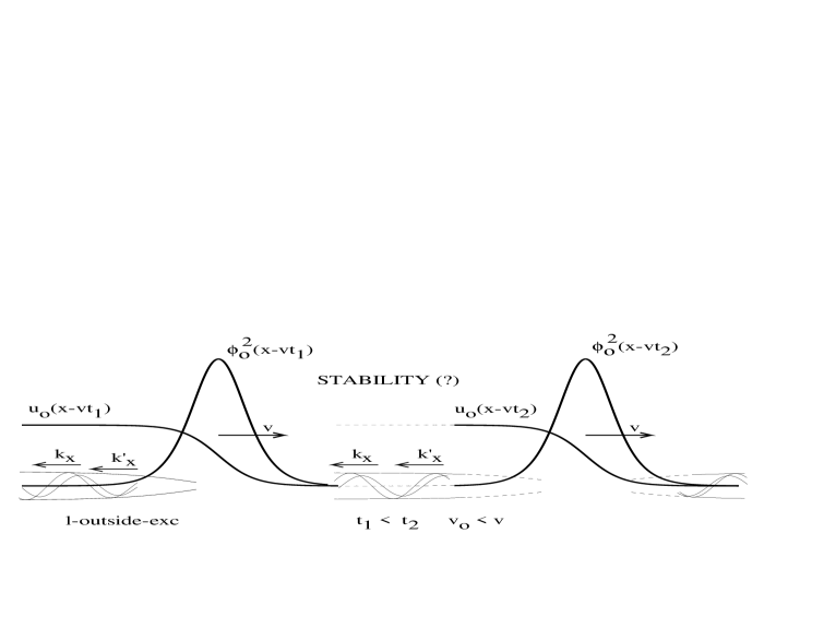
Figure 2: The ballistic condensate, $\phi_{\rm o}(x-vt)\cdot u_{\rm o}(x-vt)\delta_{1j}$, seems to be stable in relation to emission of the outside exciton-phonon excitations. (We consider the backward emission in the long-wavelength limit.) The outside-excitations presented on this figure are labeled by the wave vectors, $k_{x},\,\,k^{\prime}_{x}<0$ in the co-moving frame. In the first approximation, the outside-excitations can be described in terms of free excitons and free (acoustic) phonons emitted from the condensate coherently.

4.2 Inside-Excitations

To simplify the calculation of inside-excitation spectrum (see Eqs. (59)-(61) ) we will use the semiclassical approximation [27]. In this approximation, the excitations can be labeled by the wave vector ${\bf k}$ in the co-moving frame, and the following representation holds:

$${\rm u}_{j,s}({\bf x})={\rm u}_{j,{\bf k}}({\bf x})\,{\rm e}^{i\varphi_{\bf k}({\bf x})},\,\,\,{\rm v}_{j,s}({\bf x})={\rm v}_{j,{\bf k}}({\bf x})\,{\rm e}^{i\varphi_{\bf k}({\bf x})},\,\,\,C_{j,s}^{r}({\bf x})=C_{j,{\bf k}}^{r}({\bf x})\,{\rm e}^{i\varphi_{\bf k}({\bf x})},$$ (70)

where the phase  $\varphi_{\bf k}({\bf x})\approx\varphi_{\rm o}+{\bf kx}$, and ${\rm u}_{\bf k}({\bf x})$, ${\rm v}_{\bf k}({\bf x})$, and $C_{{\bf k}}({\bf x})$ are assumed to be smooth functions of ${\bf x}$ in the inside condensate area. Notice that the ${\bf k}$- and ${\bf x}$-representations are mixed here. This means that the operator nature of the fluctuating fields is actually dismissed within the semiclassical approximation. Howevever, the orthogonality relations among ${\rm u}_{j,s}$,  ${\rm v}_{j,s^{\prime}}$, and $C_{j,s}$,  $C_{j,s^{\prime}}^{*}$, and, hence, among  ${\rm u}_{j,{\bf k}}$,  ${\rm v}_{j,{\bf k}^{\prime}}$, and $C_{j,{\bf k}}$,  $C_{j,{\bf k^{\prime}}}^{*}$ come from the Bose commutation relations between the operators $\alpha_{j,s}$ and $\alpha^{{\dagger}}_{j,s^{\prime}}$ [26],[27]. For example, Eq. (54) is modified as follows:

$$\delta{\psi}({\bf x},t)\simeq\!\int\!\frac{d{\bf k}}{(2\pi)^{3}}\,{\rm u}_{\bf k}({\bf x}){\rm e}^{i\varphi_{\bf k}({\bf x})}{\rm e}^{-i\omega_{\bf k}({\bf x})t}\,+\,{\rm v}_{\bf k}^{*}({\bf x}){\rm e}^{-i\varphi_{\bf k}({\bf x})}{\rm e}^{i\omega_{\bf k}({\bf x})t},$$ (71)

and the inside-excitation part of the elementary excitation term in Eq. (51),
$\sum_{j,s}\cdots\approx\sum_{j,s,\,{\rm out}}+\sum_{j,s,\,{\rm surf}}+\sum_{j,s,\,{\rm in}}\cdots$, can be written as

$$\sum_{1,s,\,{\rm in}}\hbar\omega_{1,s}\hat{\alpha}_{1,s}^{{\dagger}}\hat{\alpha}_{1,s}\simeq\int\!\frac{d{\bf k}\,d{\bf x}}{(2\pi)^{3}}\,\hbar\omega_{1,{\bf k}}({\bf x})\,n_{1,{\bf k}}({\bf x}).$$ (72)

Note that the semiclassical energy $\hbar\omega_{j,{\bf k}}(x)$ of the inside-excitation mode $j,{\bf k}$ is supposed to be a smooth function of $x$ as well, (at least, as smooth as $\phi_{\rm o}^{2}(x)$, which is taken constant in the inside-approximation).

Although the low-lying excitations cannot be properly described within the semiclassical approximation, we apply it here to calculate the low-energy asymptotics of the spectrum. In fact, within the approximation $\bar{H}\approx H_{\rm o}+\bar{H}_{2}$, all the important properties of such excitations can be understood by use of the semiclassical approach.

There are two different types of the inside-excitations, the longitudinal excitations and the transverse ones. The later have the wave vectors ${\bf k}$ perpendicular to the $x\,(v)$-direction. For the sake of simplicity, we choose  ${\bf k}\parallel Oy$. Then the vector $C_{j,{\bf k}}^{r}$ has one nonzeroth component for such transverse excitations,  $C_{j,k}^{y}\neq 0$.

Substituting ansatz (70) with $k_{r}=k_{\perp}\,\delta_{2,r}$ and $C_{j,{\bf k}}^{r}=C_{j,k}^{y}\,\delta_{2,r}$ into Eqs. (59)-(61), we transform these differential equations into the algebraic ones (within the inside-approximation  $\hat{L}(\Delta)\rightarrow L(-{\bf k}^{2})$ ):

$$(L(-k_{\perp}^{2})-\hbar\omega_{j,k})\,{\rm u}_{k}({\bf x})+\left(\nu_{0}\phi_{\rm o}^{2}({x})+2\nu_{1}\phi_{\rm o}^{4}({x})\right){\rm v}_{j,k}({\bf x})+\sigma_{0}\phi_{\rm o}({x})\,ik_{\perp}{C}_{j,k}^{y}({\bf x})=0,$$ (73)

$$\left(\nu_{0}\phi_{\rm o}^{2}(x)+2\nu_{1}\phi_{\rm o}^{4}({x})\right){\rm u}_{j,k}({\bf x})+(L(-k_{\perp}^{2})+\hbar\omega_{j,k})\,{\rm v}_{j,k}({\bf x})+\sigma_{0}\phi_{\rm o}({x})\,i{k_{\perp}}{C}_{j,k}^{y}({\bf x})=0$$ (74)

$$\rho^{-1}\sigma_{0}\phi_{\rm o}(x)\,ik_{\perp}\,{\rm u}_{j,k}({\bf x})+\rho^{-1}\sigma_{0}\phi_{\rm o}(x)\,ik_{\perp}\,{\rm v}_{j,k}({\bf x})+\left[\,\omega_{j,k}^{2}-c_{l}^{2}k_{\perp}^{2}\right]C_{j,k}^{y}({\bf x})=0.$$ (75)

After some straightforward algebra, we can write out the equation that defines the spectrum of transverse exciton-phonon excitations in the inside-approximation:

$$\left(\,\omega_{j,k}^{2}-c_{l}^{2}{k_{\perp}}^{2}\right)\times$$

$$\times\left[\,(\hbar\omega_{j,k})^{2}-\left(L(-k_{\perp}^{2})-\nu_{0}\phi_{\rm o}^{2}({x})-2\nu_{1}\phi_{\rm o}^{4}({x})\,\right)\left(L(-k_{\perp}^{2})+\nu_{0}\phi_{\rm o}^{2}({x})+2\nu_{1}\phi_{\rm o}^{4}({x})\,\right)\,\right]=$$

$$=\left(\,L(-k_{\perp}^{2})-\nu_{0}\phi_{\rm o}^{2}({x})-2\nu_{1}\phi_{\rm o}^{4}({x})\,\right)\,\,\frac{2\,\sigma_{0}^{2}}{\rho\,c_{l}^{2}}\,\phi_{\rm o}^{2}(x)\,(c_{l}^{2}k_{\perp}^{2}).$$ (76)

Taking into account the momentum cut-off $k_{0}$, which is defined as

$$(\hbar^{2}/2m)\,k_{0}^{2}\approx|\tilde{\mu}|=(\hbar^{2}/2m)\,L_{0}^{-2},\,\,\,\,\,k>k_{0},$$

we can rewrite Eq. (76) as follows

$$\left(\,\omega_{j,k}^{2}\,-\,c_{l}^{2}k_{\perp}^{2}\,\right)\times$$

$$\times\left[\,(\hbar\omega_{j,k})^{2}-\left(\frac{\hbar^{2}}{2m}[k_{\perp}^{2}-{k}_{0}^{2}]+F(x)+\epsilon_{+}\right)\!\cdot\!\left(\frac{\hbar^{2}}{2m}[k_{\perp}^{2}-{k}_{0}^{2}]+F(x)+2\nu_{0}\phi^{2}_{\rm o}(x)+\epsilon_{+}^{\prime}\right)\,\right]=$$

$$=\left(\,\frac{\hbar^{2}}{2m}[k_{\perp}^{2}-k_{0}^{2}]+F(x)+\epsilon_{+}\right)\,2\frac{\sigma_{0}}{Mc_{l}^{2}}\,(\sigma_{0}a_{l}^{3})\,\Phi_{\rm o}^{2}\,(c_{l}^{2}k_{\perp}^{2}),\,\,\,\,\,\,|x|<L_{0}.$$ (77)

Here  $F(x)=|\widetilde{\nu_{0}}\,(v)|(\Phi_{\rm o}^{2}-\phi_{\rm o}^{2}(x)\,)>0$, i.e.  $F(x)\simeq 0$ inside the condensate, and

$$\epsilon_{+}\approx\widetilde{\nu_{1}}\,\phi_{\rm o}^{4}(x),\,\,\,\,\,\,\epsilon_{+}^{\prime}\approx 5{\nu_{1}}\,\phi_{\rm o}^{4}(x),\,\,\,\,\,\,k_{\perp}>k_{0}.$$

Although Eq. (77) can be solved exactly for the transverse excitation spectrum [30], taking into account the coupling term in the r.h.s. of (77) changes the values of excitation energies slightly, and the excitations can be approximately considered as of the pure excitonic ($\hbar\omega_{1,k}=\hbar\omega_{{\rm ex},\,k_{\perp}}$) or the pure phonon ($\hbar\omega_{2,k}=\hbar\omega_{{\rm ph},\,k_{\perp}}$) types.

It is also useful to investigate asymptotics of the transverse inside excitations. For definiteness sake, we investigate the left side asymptotics of these excitations here,

$${\rm u}_{j,s}({\bf x})=\exp(\ell_{u}x/L_{0})\,{\rm e}^{ik_{\perp}y}\,u_{j,k},\,\,\,\,\,\,\,{\rm v}_{j,s}({\bf x})=\exp(\ell_{v}x/L_{0})\,{\rm e}^{ik_{\perp}y}\,v_{j,k},\,\,\,\,x<0,$$ (78)

$$C_{j,s}^{y}({\bf x})=\exp(\ell_{c}x/L_{0})\,{\rm e}^{ik_{\perp}y}\,C_{j,k}^{y},\,\,\,\,\,C_{j,s}^{x}({\bf x})=\exp(\ell_{c}x/L_{0})\,{\rm e}^{ik_{\perp}y}\,C_{j,k}^{x},\,\,\,\,x<0.$$ (79)

Here  $u_{j,k}$, $v_{j,k}$, $C_{j,k}^{y}$, and $C_{j,k}^{x}$ are smooth functions of ${\bf x}$ at   $|x|>L_{0}$. Note that we introduced two components of ${C}_{j,s}^{r}\sim{\rm e}^{ik_{\perp}y}$ to make Eqs. (59)-(62) self-consistent. Let the equalities

$$\ell_{u}=\ell_{v}=1\,\,\,\,\,{\rm and}\,\,\,\,\,1+\ell_{u}=\ell_{c}=2\$$ (80)

be valid. Then the system of differential equations (59)-(62) can be reduced to a system of algebraic ones, which are analogous to Eqs. (73)-(75). Consequently, we can write out the equation for $\omega_{j,k}(x)$ valid at $|x|>L_{0}$,

$$\left(\,[\,\omega_{j,k}-iv\,(2/L_{0})\,]^{2}\,-\,c_{l}^{2}[k^{2}_{\perp}-(2/L_{0})^{2}]\,\right)\times$$

$$\times\left[\,(\hbar\omega_{j,k})^{2}-\left(\frac{\hbar^{2}}{2m}[{k}^{2}_{\perp}-\tilde{k}_{0}^{2}]+\tilde{F}(x)\right)\cdot\left(\frac{\hbar^{2}}{2m}[{k}^{2}_{\perp}-\tilde{k}_{0}^{2}]+\tilde{F}(x)+2\nu_{0}(2\Phi_{\rm o}\exp(x/L_{0})\,)^{2}\right)\,\right]=$$

$$=\left(\,\frac{\hbar^{2}}{2m}[{k}^{2}_{\perp}-\tilde{k}_{0}^{2}]+\tilde{F}(x)\,\right)\,2\frac{\sigma_{0}}{Mc_{l}^{2}}\,(\sigma_{0}a_{l}^{3})\,\bigl{(}2\Phi_{\rm o}\exp(x/L_{0})\,\bigr{)}^{2}\,c_{l}^{2}[\,k^{2}_{\perp}-(2/L_{0})^{2}],$$ (81)

where  $\tilde{k}_{0}=\sqrt{2}/L_{0}\simeq k_{0}$,  $k_{\perp}>\tilde{k}_{0}$, and

$$\tilde{F}(x)=|\widetilde{\nu_{0}}\,(v)|\left(\Phi_{\rm o}^{2}-\bigl{(}2\Phi_{\rm o}\exp(x/L_{0})\,\bigr{)}^{2}\,\right)\rightarrow 2|\tilde{\mu}|-\epsilon\,\,\,\,{\rm at}\,\,\,\,|x|\gg L_{0}.$$

(We neglected the terms, such as $\widetilde{\nu_{1}}\,\phi_{\rm o}^{4}(x)\,{\rm u}_{j,s}({\bf x})$ and  $\nu_{1}\phi_{\rm o}^{4}(x)\,{\rm v}_{j,s}({\bf x})\sim\exp\bigl{(}\,(4+\ell_{u})x/L_{0}\,\bigr{)}$ in Eqs. (59)-(60), and the terms $\propto\kappa_{3}$ in Eq. (62) as well.)

Obviously, the structure of Eqs. (77) and (81) is the same. As the coupling between exciton and phonon branches is weak for the transverse inside-excitations (see the r.h. sides of Eqs. (77) and (81) ) and the effect of the finite width $L_{0}$ can be taken into account as the spatial dependence of the important parameters in $\hbar\omega_{\rm ex}$, we use the following formula to estimate the low-energy excitation spectrum:

$$(\hbar\omega_{{\rm ex},\,k_{\perp}})^{2}\simeq\left(\frac{\hbar^{2}}{2m}(k^{2}_{\perp}-k_{0}^{2})+F(x)+\epsilon_{+}\right)\,\left(\frac{\hbar^{2}}{2m}(k^{2}_{\perp}-k_{0}^{2})+F(x)+2\nu_{0}\phi_{\rm o}^{2}(x)+\epsilon_{+}^{\prime}\right)\,\sim$$

$$\sim\,\frac{\hbar^{2}}{2m}(k^{2}_{\perp}-k_{0}^{2})\,2\nu_{0}\Phi_{\rm o}^{2}+2\nu_{0}\Phi_{\rm o}^{2}\,\epsilon_{+}\,\,\,\,\,{\rm at}\,\,\,\,\,k_{\perp}\rightarrow k_{0}.$$ (82)

Here we take the inside-condensate-asymptotics of $F(x)$, $\phi_{\rm o}^{2}(x)$, and $\epsilon_{+}\approx\widetilde{\nu_{1}}(v)\,\phi_{\rm o}^{4}(x)$ to estimate $\hbar\omega_{\rm ex}$. Note that, for the inside-condensate excitations, the the low-energy limit means

$$(\hbar^{2}/2m)(k^{2}_{\perp}-k_{0}^{2})\simeq(1\sim 10)\,|\tilde{\mu}|.$$

Then, in the co-moving frame, the low-energy excitation spectrum   $\hbar\omega_{{\rm ex}\,k_{\perp}}$  may develop a gap of the order of  $|\tilde{\mu}|$, (see Eq. (64) for comparison). Thus, inside the condensate, we obtain a strong deviation of the collective excitation spectrum from both the simple excitonic one,  $|\tilde{\mu}|+(\hbar^{2}/2m)k_{\perp}^{2}$, and the Bogoliubov-Landau spectrum  $\propto|k_{\perp}|$.

4.3 Longitudinal inside-excitations

The case of the longitudinal excitations, $k_{r}=k_{x}\,\delta_{1,r}$, $C_{j,{\bf k}}^{r}=C_{j,k}^{x}\,\delta_{1,r}$, is more difficult to analyze because the mode interaction is non-negligible in the low-energy limit. (On Fig. 1., a longitudinal inside-excitation is shown with the two possible directions of the wave vector ${\bf k}\parallel Ox$.) Recall that the “bare” phonon modes, which can be written in the laboratory frame as

$$u_{x}(x,t)\simeq q_{\rm o}(x-vt)+C_{k}^{x}(x-vt)\,{\rm exp}(ik_{x}x-i\omega_{\rm ph}t)+c.c.$$

with  $\omega_{\rm ph}=c_{l}|k_{x}|$ and $C_{k}^{x}(x)\sim\phi^{2}_{\rm o}(x)$, will be considered in the co-moving frame, $x-vt\rightarrow x$. Then, within the inside-condensate approximation, the following equation stands for the excitation spectrum:

$$\left(\,(\omega_{j,k}+vk_{x})^{2}\,-\,c_{l}^{2}k_{x}^{2}\,\right)\times$$

$$\times\left[\,(\hbar\omega_{j,k})^{2}-\left(\frac{\hbar^{2}}{2m}[k_{x}^{2}-{k}_{0}^{2}]+F(x)+\epsilon_{+}\right)\cdot\left(\frac{\hbar^{2}}{2m}[k_{x}^{2}-{k}_{0}^{2}]+F(x)+2\nu_{0}\phi^{2}_{\rm o}(x)+\epsilon_{+}^{\prime}\right)\,\right]=$$

$$=\left(\,\frac{\hbar^{2}}{2m}[k_{x}^{2}-k_{0}^{2}]+F(x)+\epsilon_{+}\right)\,2\frac{\sigma_{0}}{Mc_{l}^{2}}\,(\sigma_{0}a_{l}^{3})\,\Phi_{\rm o}^{2}\,(c_{l}^{2}k_{x}^{2}),\,\,\,\,\,\,|x|<L_{0}.$$ (83)

It is important to note that, unlike the case of transverse excitations, the values of

$$\Bigl{(}\hbar\omega_{{\rm ph},\,k_{x}}^{(0)}\Bigr{)}^{2}\simeq\hbar^{2}\,(c_{l}-v)^{2}\bigl{(}(3\sim 7)\,k_{0}\bigr{)}^{2}$$

and

$$\Bigl{(}\hbar\omega_{{\rm ex},\,k_{x}}^{(0)}\Bigr{)}^{2}\simeq\left(\frac{\hbar^{2}}{2m}(10\sim 40)k_{0}^{2}+\epsilon_{+}\right)\,\left(\frac{\hbar^{2}}{2m}(10\sim 40)k_{0}^{2}+2\,\nu_{0}\,\phi_{\rm o}^{2}(x)+\epsilon_{+}^{\prime}\right)$$

are of the same order of value at $k_{x}\simeq(3\sim 8)\,k_{0}$, and the inequality $\bigl{(}\hbar\omega_{{\rm ex},\,k_{x}}^{(0)}\bigr{)}^{2}>\bigl{(}\hbar\omega_{{\rm ph},k_{x}}^{(0)}\bigr{)}^{2}$ is valid in the low-energy limit. Moreover, the two cases, $k_{x}>0$ ($+$ - case) and $k_{x}<0$ ($-$ - case), are different as it can be seen from the l.h.s. of Eq. (83). In the low-energy limit, we can write the approximate solution of (83) as follows

$$\Bigl{(}\hbar\omega_{{\rm ex},\,k_{x}}^{(\pm)}\Bigr{)}^{2}\approx\left(\frac{\hbar^{2}}{2m}[k_{x}^{2}-{k}_{0}^{2}]+F(x)+\epsilon_{+}\right)\times$$

$$\times\left(\frac{\hbar^{2}}{2m}[k_{x}^{2}-{k}_{0}^{2}]+F(x)+2\nu_{0}\,\phi^{2}_{\rm o}(x)\pm 2\,q_{\pm}\gamma(v)\,\frac{\sigma_{0}}{Mc_{l}^{2}}\,(\sigma_{0}a_{l}^{3})\,\phi_{\rm o}^{2}(x)+\epsilon_{+}^{\prime}\right),$$

where $q_{+}\sim 1$ and $0<q_{-}<1$. Note that $\hbar\omega^{(+)}_{{\rm ex},\,k_{x}}>\hbar\omega_{{\rm ex},\,k_{x}}^{(0)}$, whereas, for the phonon-type branch, $\omega^{(+)}_{{\rm ph},\,k_{x}}<\,(c_{l}-v)\,k_{x}$. For $k_{x}<0$, we have the following inequaluty for the excitonic branch,

$$\left(\frac{\hbar^{2}}{2m}[k_{x}^{2}-{k}_{0}^{2}]+F(x)+\epsilon_{+}\right)\times$$

$$\times\left(\frac{\hbar^{2}}{2m}[k_{x}^{2}-{k}_{0}^{2}]+F(x)+2\,\widetilde{\nu_{0}}(v)\,\phi^{2}_{\rm o}(x)+\epsilon_{+}^{\prime}\right)<\Bigl{(}\hbar\omega^{(-)}_{{\rm ex},\,k_{x}}\Bigr{)}^{2}<\Bigl{(}\hbar\omega_{{\rm ex},\,k_{x}}^{(0)}\bigr{)}^{2},$$ (84)

where $2\,\widetilde{\nu_{0}}(v)\,\phi^{2}_{\rm o}(x)\simeq-4\,|\tilde{\mu}|$ within the inside-approximation, and, for the phonon-type branch, we obtain $\omega^{(-)}_{{\rm ph},\,k_{x}}>\,(c_{l}+v)\,|k_{x}|$.

To derive the formulas for the amplitudes  ${\rm u}_{k}({x})$,  ${\rm v}_{k}({x})$, and  ${C}_{k}^{x}({x})$ of the excitonic branch, we use the following approximations

$$L_{\pm}(-{k}_{x}^{2})=L(-{k}_{x}^{2})+\frac{\rho^{-1}\sigma_{0}^{2}\phi_{\rm o}^{2}(x)\,k_{x}^{2}}{(\omega_{{\rm ex},\,k_{x}}\pm v|k_{x}|)^{2}-c_{l}^{2}k_{x}^{2}}\approx L(-{k}_{x}^{2})\,\pm\,q_{\pm}\gamma(v)\,\frac{\sigma_{0}}{Mc_{l}^{2}}\,(\sigma_{0}a_{l}^{3})\,\phi_{\rm o}^{2}(x),$$

and $B=\nu_{0}\phi_{\rm o}^{2}({x})+2\nu_{1}\phi_{\rm o}^{4}({x})$ is modified as

$$B_{\pm}\approx\nu_{0}\phi_{\rm o}^{2}({x})+2\nu_{1}\phi_{\rm o}^{4}({x})\pm q_{\pm}\gamma(v)\,\frac{\sigma_{0}}{Mc_{l}^{2}}\,(\sigma_{0}a_{l}^{3})\,\phi_{\rm o}^{2}(x).$$

Then we can rewrite the formulas for the excitonic excitation spectrum as follows

$$\bigl{(}\hbar\omega_{{\rm ex},\,k_{x}}^{(\pm)}\bigr{)}^{2}\approx L_{\pm}^{2}(-{k}_{x}^{2})-B_{\pm}^{2}=\Bigl{(}L(-{k}_{x}^{2})-B\Bigr{)}\Bigl{(}L_{\pm}(-{k}_{x}^{2})+B_{\pm}\Bigr{)}.$$

Recall that the orthogonality relation (58) can be used to normalize the amplitudes. Within the inside-approximation, Eq. (58) can be rewritten as follows ($\delta_{ss}=1\rightarrow\delta_{kk}=1$)

$$\int\!d{\bf x}\,\bigl{(}|{\rm u}_{k}({x})|^{2}-|{\rm v}_{k}({x})|^{2}\,\bigr{)}\,+\,(1/\hbar)\!\int\!d{\bf x}\,2\rho\,(\omega_{{\rm ex},\,k_{x}}+vk_{x})|C_{k}^{x}(x)|^{2}=1,$$ (85)

and we have for the excitonic amplitudes

$$\Bigl{|}{\rm u}_{k}^{(\pm)}(x)\Bigr{|}^{2}\approx\left(\frac{\Upsilon_{\pm}}{V_{\rm eff}}\right)\frac{L_{\pm}(-k_{x}^{2})+\hbar\omega_{{\rm ex},\,k_{x}}^{(\pm)}}{2\,\hbar\omega_{{\rm ex},\,k_{x}}^{(\pm)}},\,\,\,\,\,\Bigl{|}{\rm v}_{k}^{(\pm)}(x)\Bigr{|}^{2}\approx\left(\frac{\Upsilon_{\pm}}{V_{\rm eff}}\right)\frac{L_{\pm}(-k_{x}^{2})-\hbar\omega_{{\rm ex},\,k_{x}}^{(\pm)}}{2\,\hbar\omega_{{\rm ex},\,k_{x}}^{(\pm)}},$$ (86)

$${\rm u}_{k}^{(\pm)\,*}{\rm v}_{k}^{(\pm)}(x)\approx-\left(\frac{\Upsilon_{\pm}}{V_{\rm eff}}\right)\frac{B_{\pm}}{2\,\hbar\omega_{{\rm ex},\,k_{x}}^{(\pm)}}.$$

Here the effective condensate volume $V_{\rm eff}\simeq 2SL_{0}$ is used to normalize the u- and v-wave functions of the inside excitations, and  $\int\!\!d{\bf r}\,(|{\rm u}_{k}|^{2}-|{\rm v}_{k}|^{2})=\Upsilon_{\pm}<1$.

Subsiquently, we get for

$$C_{k}^{x}(x)=-\frac{\rho^{-1}\sigma_{0}\,\phi_{\rm o}(x)\,ik_{x}\,\bigl{(}{\rm u}_{k}(x)+{\rm v}_{k}(x)\,\bigr{)}}{(\omega_{{\rm ex},\,k_{x}}+vk_{x})^{2}-c_{l}^{2}{k}^{2}}$$ (87)

the following approximate formulas

$$C_{k}^{x\,(\pm)}(x)\approx\mp\,q_{\pm}\,\gamma(v)\,\frac{\sigma_{0}}{Mc_{l}^{2}}\,\sqrt{a_{l}^{3}\,\phi_{\rm o}^{2}(x)}\,\frac{i}{k_{x}}\,\sqrt{a_{l}^{3}}\,\bigl{(}{\rm u}_{k}^{(\pm)}(x)+{\rm v}_{k}^{(\pm)}(x)\,\bigr{)}.$$

To estimate the characteristic value of  $C_{k}^{x\,(\pm)}(x)$, we use ${\rm u}_{k}(x)\simeq{\rm v}_{k}(x)\sim\sqrt{\Upsilon_{\pm}/V_{\rm eff}}$ and obtain

$$|C_{k}^{x\,(\pm)}|\simeq q_{\pm}\,\gamma(v)\,\frac{\sigma_{0}}{Mc_{l}^{2}}\,\sqrt{a_{l}^{3}\,\Phi_{\rm o}^{2}}\,\sqrt{\frac{\Upsilon_{\pm}\,a_{l}\,L_{0}}{2S}}\,\frac{a_{l}}{(3\sim 7)}<\!\!<\!\!<a_{l}.$$

The parameters $\Upsilon_{\pm}$ characterize the relative weight of excitonic degrees of freedom in the considered branch of excitations. As the parameter  $\hbar vk_{x}/\hbar\omega_{{\rm ex},\,k_{x}}^{(+)}<1$ at  $k_{x}\simeq(4\sim 8)\,k_{0}$, the parameter  $\Upsilon_{+}(k_{x})$  can be estimated as $0.5\sim 0.7$. For $k_{x}<0$, we obtain the following equation from (85),

$$\Upsilon_{-}\,\left(1+\frac{\bigl{(}a_{l}^{3}\,\Phi_{\rm o}^{2}\bigr{)}}{m/M}\,q_{-}^{2}\,\gamma^{2}(v)\,\Bigl{(}\frac{\sigma_{0}}{Mc_{l}^{2}}\Bigr{)}^{2}\left(1-\frac{\hbar v|k_{x}|}{\hbar\omega_{{\rm ex},\,k_{x}}^{(-)}}\right)\frac{L(-{k}_{x}^{2})-B}{\hbar^{2}k_{x}^{2}/2m}\,\right)\approx 1.$$

Within the stability area (see the next subsection for an extended discussion), we estimate the ratio $\hbar v|k_{x}|/\hbar\omega_{{\rm ex},\,k_{x}}^{(-)}\simeq 1/2\sim 1/3$ at  $|k_{x}|\simeq(4\sim 8)\,k_{0}$. Then,   $\Upsilon_{-}(k_{x})>0$ and  $\Upsilon_{-}\simeq 0.6\sim 0.8$.

To go beyond the inside-approximation, the effect of inhomogeneous behavior of the longitudinal excitations can be considered. We use the following ansatz for the left side asymptotics (see Fig. 2)

$${\rm u}_{j,s}({\bf x})=\exp(\ell_{u}x/L_{0})\,{\rm e}^{ik_{x}x}\,u_{k},\,\,\,\,\,\,\,{\rm v}_{j,s}({\bf x})=\exp(\ell_{v}x/L_{0})\,{\rm e}^{ik_{x}x}\,v_{k},$$ (88)

$$C_{j,s}^{x}({\bf x})=\exp(\ell_{c}x/L_{0})\,{\rm e}^{ik_{x}x}\,C_{k}^{x},\,\,\,\,\,\,x<0.$$ (89)

where  $\ell_{u}=\ell_{v}=1$  and  $\ell_{c}=2$. Then, like the case of transversal excitations (see Eq. (81)), we can write the equation for $\omega_{j,\,k_{x}}(x)$ valid at $|x|>L_{0}$,

$$\left(\,(\,\omega_{j,\,k_{x}}+v\,\tilde{k}_{x})^{2}\,-\,c_{l}^{2}\tilde{k}^{2}_{x}\,\right)\times$$

$$\times\left[\,(\hbar\omega_{j,\,k_{x}})^{2}-\left(\frac{\hbar^{2}}{2m}[\bar{k}^{2}_{x}-{k}_{0}^{2}]+\tilde{F}(x)\right)\left(\frac{\hbar^{2}}{2m}[\bar{k}^{2}_{x}-{k}_{0}^{2}]+\tilde{F}(x)+2\nu_{0}\bigl{(}2\Phi_{\rm o}\exp(x/L_{0})\,\bigr{)}^{2}\right)\,\right]=$$

$$=\left(\,\frac{\hbar^{2}}{2m}[\bar{k}^{2}_{x}-{k}_{0}^{2}]+\tilde{F}(x)\,\right)\,2\frac{\sigma_{0}}{Mc_{l}^{2}}\,(\sigma_{0}a_{l}^{3})\,\bigl{(}2\Phi_{\rm o}\exp(x/L_{0})\,\bigr{)}^{2}\,c_{l}^{2}\tilde{k}^{2}_{x},$$ (90)

where $k_{x}\rightarrow\tilde{k}_{x}=k_{x}-i(2/L_{0})$ in the phonon parts of this equation and $k_{x}\rightarrow\bar{k}_{x}=k_{x}-i(1/L_{0})$ in the exciton parts of it ($x<0$). It is easy to see that Eqs. (83) and (90) are in the continuity correspondence, i.e. they describe the same object. For example, the (left side) asymptotic behavior of $\hbar\omega_{{\rm ex},\,k_{x}}^{(\pm)}(x)$ can be obtained from the inside-condensate formulas by the substitute

$$k_{x}\rightarrow\bar{k}_{x},\,\,\,\,\,F(x)\rightarrow\tilde{F}(x)\rightarrow 2|\tilde{\mu}|,$$

and

$$\phi_{\rm o}^{2}(x)\rightarrow(2\Phi_{\rm o}\exp(x/L_{0})\,)^{2}\rightarrow 0.$$

As a result, we obtain $\hbar\omega_{{\rm ex},\,k_{x}}\simeq|\tilde{\mu}|+\hbar^{2}\bar{k}^{2}_{x}/2m$ that corresponds to the outside-excitation spectrum, Eq. (63).

The excitonic input into $\langle\delta\hat{\Psi}^{{\dagger}}\delta\hat{\Psi}({\bf x})\rangle_{T=0}$, the quantum depletion of the moving condensate, can be calculated by $\sum_{1,s}|{\rm v}_{1,s}(x)|^{2}$ [27]. To estimate this value, one can approximate $|{\rm v}_{k}(x)|^{2}$ as follows

$$\Bigl{|}{\rm v}_{k_{x}}^{(\pm)}(x)\Bigr{|}^{2}\simeq\left(\frac{\Upsilon_{\pm}}{V_{\rm eff}}\right)\frac{B_{\pm}^{2}}{4L_{\pm}^{2}(-k_{x}^{2})}.$$

However, the summation $\sum_{1,s}$  implies  $\int\!dk_{x}\,d^{2}k_{\perp}/(2\pi)^{3}$ within the semiclassical approximation. Assuming that such an integration makes the difference among ${\rm v}_{k_{x}}^{(-)}$,  ${\rm v}_{k_{x}}^{(+)}$  and  ${\rm v}_{k_{\perp}}$ not essentially important, we use the following estimate for $|{\rm v}_{\bf k}(x)|^{2}$,

$$\Bigl{|}{\rm v}_{\bf k}(x)\Bigr{|}^{2}\simeq\left(\frac{1}{V_{\rm eff}}\right)\frac{B^{2}}{4L^{2}(-{\bf k}^{2})}.$$

Then, the integration $\int\!dk_{x}\,d^{2}k_{\perp}/(2\pi)^{3}$ can be reduced to $\int_{k_{0}}\!k^{2}dk/2\pi^{2}$, and the main input ($\sim\phi_{\rm o}^{2}(x)$) can be estimated from the following formula

$$\langle\delta\hat{\Psi}^{{\dagger}}\delta\hat{\Psi}({\bf x})\rangle_{T=0}\,\simeq\frac{1}{8\pi^{2}\,L_{0}^{3}}\,\frac{\nu_{0}\phi_{\rm o}^{2}(x)}{2|\tilde{\mu}|}+\frac{\epsilon}{8\pi^{2}\,L_{0}^{3}}\,\frac{\bigl{(}\nu_{0}\phi_{\rm o}^{2}(x)\,\bigr{)}^{2}}{2|\tilde{\mu}|^{2}}\sim\frac{1}{8\pi^{2}\,L_{0}^{3}}\,\frac{\nu_{0}\Phi_{\rm o}^{2}\,{\rm cosh}^{-2}(x/L_{0})}{|\widetilde{\nu_{0}}|\,\Phi_{\rm o}^{2}}.$$

Using this density, we speculate that the localized depletion of condensate – i.e. the number of particles that are out of the condensate but move with it coherently – seems to be a small value. We obtain the following estimate ($\nu_{0}=\varepsilon_{0}\,\tilde{a}_{B}^{3}$  and  $|\widetilde{\nu_{0}}(v)|=|\tilde{\varepsilon}_{0}(v)|\,\tilde{a}_{B}^{3}$):

$$\delta N_{0}=\int\!d{\bf x}\,\langle\delta\hat{\Psi}^{{\dagger}}\delta\hat{\Psi}({\bf x})\rangle_{T=0}\,\simeq\,\frac{1}{16\,\pi^{2}}\,\frac{\varepsilon_{0}}{|\tilde{\mu}|}\,\frac{\tilde{a}_{B}^{3}}{L_{0}^{3}}\,N_{\rm o},$$

where the factor before $N_{\rm o}$ can be estimated as

$$\frac{\varepsilon_{0}}{|\tilde{\mu}|(N_{\rm o},\,v)}\,\frac{\tilde{a}_{B}^{3}}{L_{0}^{3}(N_{\rm o},\,v)}\simeq\frac{\varepsilon_{0}\,|\tilde{\varepsilon}_{0}(v)|}{2\,x\,({\rm Ry}^{*})^{2}}\,\frac{1}{\bar{n}_{\rm o}}\sim(10^{-1}\sim 10^{-2})\,\bar{n}_{\rm o}^{-1}.$$

(Here we used Eqs. (35),(36) within the approximation  $\bar{n}_{\rm o}\gg 10$.) Note that there is no small ${\bf k}$ input to the estimate of $\sum_{1,s}$ because, first, such excitations belong to the outside-excitation branch in our model, and, second, we use the approximation  ${\rm v}_{\bf k}(x)\approx 0$ for them.

4.4 Stability of the Moving Condensate

To investigate the stability of the moving condensate in relation to the creation of inside-excitations, we calculate the energy of the condensate with the one inside excitation, $\langle\alpha^{{\dagger}}_{1,s}\alpha_{1,s}\rangle=1$, described by the following set: $k$, $\omega_{k}$, and ${\rm u}_{k}$, ${\rm v}_{k}$, $C_{k}$. In this study, we analyze the stability inside the excitonic sector of our model.

Although the excitations were defined in the co-moving frame, calculations should be done in the laboratory frame. Returning to the lab frame, we represent the exciton and phonon field functions as follows:

$$\phi_{\rm o}(x-vt,\,t)\rightarrow\phi_{\rm o}(x-vt,\,t)+\exp\bigl{(}-i(\tilde{E}_{g}+mv^{2}/2-|\tilde{\mu}|)t\,\bigr{)}\exp\bigl{(}i(\varphi+mvx)\,\bigr{)}\,\delta\tilde{\Psi}({\bf x},t),$$ (91)

where

$$\delta\tilde{\Psi}({\bf x},t)={\rm u}_{k}(x-vt)\,{\rm e}^{i(\varphi_{0}+{\bf k}{\bf x})}\,{\rm e}^{-i(\omega_{k}+k_{x}v)t}+{\rm v}_{k}(x-vt)\,{\rm e}^{-i(\varphi_{0}+{\bf k}{\bf x})}\,{\rm e}^{i(\omega_{k}+k_{x}v)t},$$

and

$$u_{\rm o}(x-vt)\rightarrow u_{\rm o}(x-vt)+C_{k}(x-vt)\,\exp\bigl{(}i(\varphi_{0}+{\bf k}{\bf x})\bigr{)}\,\exp\bigl{(}-i(\omega_{k}+k_{x}v)\,t\bigr{)}+{\rm c.c.},$$ (92)

see Eq. (64) for comparison. In this analysis, the inside excitations are not considered as fluctuations, and the (average) number of particles in the condensate and its energy are changed as $N_{\rm o}-\int\!d{\bf x}\,\delta\psi^{{\dagger}}\delta\psi$ and  $E_{\rm o}(N_{\rm o})-(\partial_{N}E_{\rm o})\int\!d{\bf x}\,\delta\psi^{{\dagger}}\delta\psi$, respectively. However, these changes are not important if the number of excitation in a system is less than $\sqrt{\delta N^{2}}\simeq\sqrt{N_{\rm o}}$. They could be important in the case of instability of the moving condensate.

The zeroth component of the energy-momentum tensor can be represented in the form

$${\cal T}_{0}^{0}={\cal T}_{0}^{0}(\phi_{\rm o},\,u_{\rm o})+{\cal T}_{0}^{0\,(2)}(\delta\Psi^{{\dagger}},\delta\Psi,\delta u,\,\partial_{t}\delta u\,|\,\phi_{\rm o},\,u_{\rm o}),$$

where the first part corresponds to the condensate energy $E_{\rm o}$ and the second part gives the energy of inside-excitations, $E_{\rm in}$. After substitution of (91),(92) into $E_{\rm in}=\int\!d{\bf x}\,{\cal{T}}_{0}^{0\,(2)}$, we have for the total energy

$$E_{\rm o}+E_{\rm in-ex}\,\approx$$

$$\approx\,E_{\rm o}(N_{\rm o})+\delta E_{\rm o}(N_{\rm o})+\int\!\!d{\bf x}\,\hbar(\omega_{k}(x)+k_{x}v)\,\left\{|{\rm u}_{k}|^{2}-|{\rm v}_{k}|^{2}+(2/\hbar)\rho(\omega_{k}(x)+vk_{x})|C_{k}|^{2}\right\}\,=$$

$$=\,E_{\rm o}(N_{\rm o})+\delta E_{\rm o}(N_{\rm o})+\hbar\,\langle\omega_{k}+k_{x}v\rangle,$$ (93)

where

$$\delta E_{\rm o}(N_{\rm o})=(2|\tilde{\mu}|+\nu_{0}\Phi_{\rm o}^{2})\int\!\!d{\bf x}\,\delta\tilde{\psi}^{{\dagger}}\delta\tilde{\psi}-\frac{M(c_{l}^{2}+v^{2})}{2}\,3\vartheta(N_{\rm o},\,v)\int\!\!d{\bf x}\,\delta\tilde{\psi}^{{\dagger}}\delta\tilde{\psi},$$ (94)

$$\delta\tilde{\psi}^{{\dagger}}\delta\tilde{\psi}(x)\rightarrow|{\rm u}_{k}|^{2}+|{\rm v}_{k}|^{2},$$

see Eqs. (65),(67) for comparison.

In this study, we discuss qualitatively the stability of the condensate in relation to the backward emission of inside-excitations, (i.e. $k_{x}<0$ in the co-moving frame). To begin with, we consider the standard criterion,

$$\hbar(\omega^{(-)}_{{\rm ex},\,k}-|k_{x}|v)>0\,\,\,\,\,{\rm at}\,\,\,\,\,\,|k_{x}|\simeq z\,L_{0}^{-1},$$ (95)

where $z\simeq 3\sim 10$ corresponds to the low-lying excitations. The value of $\omega^{(-)}_{{\rm ex},\,k}(x)$ is taken within the inside-approximation, see Eq. (84), so that $\hbar\omega^{(-)}_{{\rm ex},\,k}\simeq f(z)\,|\tilde{\mu}|$ and  $z/f(z)\simeq 0.1\sim 0.3$. Then, it is easy to conclude that the following inequality

$$\frac{\hbar|k_{x}|v}{\hbar\omega^{(-)}_{{\rm ex},\,k}}\simeq\frac{z}{f(z)}\,\frac{v}{c_{l}}\,\sqrt{\frac{(4m/M)\,Mc_{l}^{2}/2}{|\tilde{\mu}|(N_{\rm o},\,v)}}<1$$ (96)

is valid in the low-energy limit if the effective chemical potential (36) is large enough, see Eq. (69) for comparison.

More precisely, the ballistic velocity $v$ and the number of particles in the condensate, $N_{\rm o}$, have to be large enough, f.ex., $|\tilde{\varepsilon}_{\rm o}(v)|\simeq(10^{-1}\sim 1)\,{\rm Ry}^{*}$ and $\bar{n}_{\rm o}\simeq 10$, in order to the inequality

$$\frac{(4m/M)\,Mc_{l}^{2}/2}{|\tilde{\mu}|(N_{\rm o},\,v)}\simeq\frac{(4m/M)\,Mc_{l}^{2}/2}{|\tilde{\varepsilon}_{\rm o}(v)|^{2}\,/\,4\bar{n}_{\rm o}^{2}\,x\,{\rm Ry}^{*}}<10\sim 20$$ (97)

can be satisfied. Thus, for

$$|\tilde{\mu}|(N_{\rm o},\,v)>\mu_{\rm cr}\simeq 10^{-1}\,(4m/M)\,Mc_{l}^{2}/2,$$ (98)

where $\mu_{\rm cr}\sim 10^{-4}$ eV, one can expect conditions (96),(97) to be valid.

Despite the condensate can be formed near $\gamma(v)\approx\gamma_{\rm o}$ in theory, f.ex., with $|\widetilde{\nu_{0}}(v)|\simeq 0.1\,\nu_{0}$ and $\bar{n}_{\rm o}\gg 10$, such a ballistic state seems to be unstable against the creation of inside-excitations. Note that the critical (Landau) velocity, $v_{\rm cr}$, can be found as a solution of Eq. (98) and $v_{\rm o}<v_{\rm cr}(N_{\rm o})<c_{l}$. In fact, the parameter $|\tilde{\mu}|/\mu_{\rm cr}$ controls the stability/instability of the condensate, see Eqs. (69),(96).

Analyzing (95), we did not take into account Eq. (94). However, if the instability regime takes place, more than $\sqrt{N_{\rm o}}$ inside-excitations can appear. As the changes in $u_{\rm o}(x-vt)$ because of $N_{\rm o}\rightarrow N_{\rm o}-\delta N$ are nonlocal (in spite of creation of the localized excitations, see Figs. 1 and 3), a free acoustic phonon can appear in the system lattice $+$ excitons together with appearance of the localized excitation $\hbar\omega^{(-)}_{{\rm ex},\,k}(x)$. Like the case of outside-excitations, we assume that $(3/2)\,M(c_{l}^{2}+v^{2})\,\vartheta(N_{\rm o},\,v)\sim\hbar c_{l}k_{\rm ph}$, see Eq. (94). Then, only the term $\propto 2|\tilde{\mu}|+\nu_{0}\Phi_{\rm o}^{2}$ is important. In fact, this term leads to some renormalization of the values of the critical parameters, $\mu_{\rm cr}$ and $v_{\rm cr}$.

Figure 3: The ballistic condensate, $\phi_{\rm o}(x-vt)\cdot u_{\rm o}(x-vt)\delta_{1j}$, can be unstable in relation to emission of the inside-excitations if the effective chemical potential $|\tilde{\mu}|(N_{\rm o},\,v)\,<\,\mu_{cr}$. In terms of Landau critical velocity, this means $v_{\rm o}<v<v_{\rm cr}(N_{\rm o})$. If such an instability takes place, the emission of inside-excitations can be accompanied by the emission of outside-excitations of the condensate. The longitudinal inside-excitations are labeled by the wave vector $k_{x}<0$ on this figure, whereas the outside-excitation is labeled by the wave vector $k^{\prime}_{x}<0$.

5 Interference Between Two Moving Packets

In this section, we address the problem of interaction between two moving condensates. This problem is essentially nonstationary, especially if the initial ballistic velocities of packets are different. Within the quasi-1D conserving model, the following equations govern the dynamics of the two input packets (we choose the reference frame moving with the slow packet):

$$\Bigl{(}\,i\hbar\partial_{t}+\frac{m(v^{\prime})^{2}}{2}\,\Bigr{)}\psi_{0}(x,t)=\Bigl{(}-\frac{\hbar^{2}}{2m}\partial^{2}_{x}+\nu_{0}|\psi_{0}|^{2}+\nu_{1}|\psi_{0}|^{4}\Bigr{)}\,\psi_{0}(x,t)+\sigma_{0}\,\partial_{x}u_{0}(x,t)\,\psi_{0}(x,t),$$ (99)

$$\bigl{(}\,(\partial_{t}-v^{\prime}\,\partial_{x})^{2}-c_{l}^{2}\partial_{x}^{2}\bigr{)}\,u_{0}(x,t)-c_{l}^{2}\,2\kappa_{3}\,\partial_{x}^{2}u_{0}(x,t)\,\partial_{x}u_{0}(x,t)=\rho^{-1}\sigma_{0}\,\partial_{x}|\psi_{0}|^{2}(x,t).$$ (100)

Then, the initial conditions can be written in the explicit 1D form by using the exact solution of the model (10),(11). Note that the amplitudes of the stationary ballistic state, $\phi_{\rm o}(x-vt)\cdot\partial_{x}u_{\rm o}(x-vt)$, were defined from the normalization condition and depend on the values of $v$ and $N_{\rm o}$. Hence, the amplitudes of the “input” condensates for Eqs. (99),(100) may not have the same values.

Figure 4: Two ballistic condensates move with different velocities, $v-v^{\prime}\simeq(0.1\sim 0.3)\,c_{l}$,  and  $t=t_{1}$ before the “collision”, or, the strong interaction process. If one can prescribe the coherent phase to each of the participating condensates, e.g., $\varphi_{\rm c}({\bf x})\approx\varphi+(mv/\hbar)\,x$, the interference area appears between them. (The interference area is marked by bold dashed lines on this figure.) As $v\neq v^{\prime}$, the fringes are non-stationary, and the outside-excitations can actually be excited in this area.

In this study, we approach the problem of strong interaction between the condensates. Therefore, we choose the nonsymmetric initial conditions, i.e. the amplitude and the velocity of the “input” packets are different, for example, $v>v^{\prime}$ and ${\bf v}\|{\bf v}^{\prime}$, see Fig. 4. Here, we reply on the experimental observation [6] that, at $v>v_{\rm o}$, the ballistic velocity of the condensate depends on the power of a laser beam irradiating the crystal. If the exciton concentration in the first packet, $n_{{\rm o}\,1}$, is close to the value of the Bose condensation threshold, the exciton concentration in the second packet, $n_{{\rm o}\,2}>n_{{\rm o}\,1}$, the velocity difference between condensates can reach $(0.1\sim 0.3)\,c_{l}$. Then, in the reference frame moving with the first (slow) packet, the initial conditions can be taken as the following:

$$\psi_{0}({x},t=0)\cdot{u}_{0}({x},t=0)=\phi_{\rm o}(x;N_{{\rm o}\,1})\cdot{q}_{\rm o}({x};N_{{\rm o}\,1})\,+\,$$

$$+\exp\bigl{(}i(\delta\varphi+m\,\delta v\,x)\bigr{)}\,\phi_{\rm o}({x}+{x}_{0};N_{{\rm o}\,2})\cdot{q}_{\rm o}({x}+{x}_{0};N_{{\rm o}\,2}),$$ (101)

where $\delta\varphi=\varphi-{\varphi}^{\prime}$, $\delta{v}={v}-{v}^{\prime}$, $x_{0}=v^{\prime}\tau$, and $\tau$ is the (initial) time delay. As the second packet moves in this frame of reference, the regime of strong nonlinear interaction between the condensates is (theoretically) unavoidable. Note that, even before collision, a time-dependent interference term in $|\psi_{\rm o}(x,t)|^{2}$ begins to influence the packet dynamics, see Fig. 4. For example, the r.h.s. of (100) contains

$$\sim\partial_{x}\left\{\,2\,{\rm cos}(m\,\delta{v}x-\delta\omega\,t+\delta\varphi)\,\phi_{\rm o}({x};N_{{\rm o}\,1})\,\phi_{\rm o}(x-\delta{v}t+x_{0};N_{{\rm o}\,2})\,\right\},$$ (102)

where

$$\hbar\delta\omega=m\,\delta{v}(v+v^{\prime})/2-\left(\,|\tilde{\mu}|(N_{{\rm o}\,2},v)-|\tilde{\mu}|(N_{{\rm o}\,1},v^{\prime})\,\right)$$

and $|\tilde{\mu}|\propto(\,N_{\rm o}/N_{\rm o}^{*})^{2}\,|\tilde{\varepsilon}_{0}(v)|^{2}$. The ratio $|\tilde{\mu}_{2}|/|\tilde{\mu}_{1}|$ can be of the order of $10^{1}$, and the characteristic scale of fringes (102) is

$$\frac{\pi(\hbar/m\,\delta v)}{L_{0}}\simeq(10\sim 30)\sqrt{\frac{|\tilde{\mu}|(N_{{\rm o}\,1},v)}{(m/M)\,Mc_{l}^{2}/2}}\simeq 5\sim 10,$$

that is they are of the long-wavelength nature.

To answer the question which model (conserving (99),(100) or kinetic [19],[32] one) is more adequate to describe the packet collision, we have to compare the estimate of interaction time,

$$\tau^{*}\simeq L_{{\rm ch}\,2}/\delta v\sim 10^{3}\,\tilde{a}_{B}/0.2\,c_{l}\simeq 10^{-9}\sim 10^{-10}\,{\rm s},$$

and characteristic time scales of the processes

$$|N_{{\rm o}\,2}(t),v\rangle\cdot|N_{{\rm o}\,1}(t),v^{\prime}\rangle\,\rightarrow\,|N_{{\rm o}\,2}(t)\pm\delta N,v\rangle\cdot|N_{{\rm o}\,1}(t)\mp\delta N,v^{\prime}\rangle$$ (103)

driven by phonons or by $x-x$ interaction. Note that some thermal phonons have to be excited in the system to assist such transitions, and the value of $\tau^{*}$ is of the order of scattering time of the exciton-LA-phonon interaction (although without any macroscopical occupancy) [17].

If processes (103) are driven by the lattice phonons, two phonons are necessary to satisfy the laws of conservation. For instance, we choose $\delta N=+1$ in (103) and obtain (see Eqs. (65),(66))

$$\hbar k_{1,\,x}=m\delta v+3Mv\,\vartheta(N_{{\rm o}\,2},\,v)-3Mv^{\prime}\,\vartheta(N_{{\rm o}\,1},\,v^{\prime})+\hbar k_{2,\,x},$$

$$\hbar c_{l}|k_{1,\,x}|=m\delta v\,(v+v^{\prime})/2-3\left(\,|\tilde{\mu}|(N_{{\rm o}\,2},\,v)-|\tilde{\mu}|(N_{{\rm o}\,1},\,v^{\prime})+\nu_{0}\,\Phi_{\rm o\,2}^{2}/3-\nu_{0}\,\Phi_{\rm o\,1}^{2}/3\right)\,+$$

$$+\,3/2\,M(c_{l}^{2}+v^{2})\,\vartheta(N_{{\rm o}\,2},\,v)-3/2\,M(c_{l}^{2}+v^{\prime 2})\,\vartheta(N_{{\rm o}\,1},\,v^{\prime})+\hbar c_{l}|k_{2,\,x}|.$$

Although the second packet moves faster, $m\delta v>0$, this state can be considered as a more stable (and, thus, more preferable) one for the excitons of the slow packet. Indeed, the following inequality for the effective difference between the generalized chemical potentials seems to be valid

$$m\delta v\,(v+v^{\prime})/2-3\left(\,|\tilde{\mu}|(N_{{\rm o}\,2},\,v)-|\tilde{\mu}|(N_{{\rm o}\,1},\,v^{\prime})+\nu_{0}\,\Phi_{\rm o\,2}^{2}/3-\nu_{0}\,\Phi_{\rm o\,1}^{2}/3\right)<0,$$ (104)

and the absolute value of the l.h.s. of (104) is $\sim|\tilde{\mu}|(N_{{\rm o}\,2}\,v)$.  Thus, within the quantum kinetic model, the relevant transition probabilities have to be calculated at least in the second order of perturbation theory, f.ex.,

$$|N_{{\rm o}\,2},v\rangle\cdot|N_{{\rm o}\,1},v^{\prime}\rangle\,\stackrel{{\scriptstyle{\rm ph}_{1}}}{{\longrightarrow}}\,|N_{{\rm o}\,2},v\rangle\cdot|N_{{\rm o}\,1},\,\hbar\omega_{{\rm ex},\,k_{j}},\,v^{\prime}\rangle\,\stackrel{{\scriptstyle{\rm ph}_{2}}}{{\longrightarrow}}\,|N_{{\rm o}\,2}+2,v\rangle\cdot|N_{{\rm o}\,1}-2,v^{\prime}\rangle.$$

As a result, the system of two quantum Boltzmann equations will describe the interaction process.

Unlike the Boltzmann equations, Eqs. (99, 100) contain information about the quantum coherence between two condensates explicitly and, moreover, can describe the case of strong interaction. Unlike the 1D NLS equation that supports many-soliton solutions, Eqs. (99),(100) are, in fact, quasi-1D ones, and $\nu_{0}>0$ in (99). Therefore, it is an open question what happens with two (excitonic) solitons after they collide in the crystal.

In this work, we assume that the dominant process(es) of condensate interactions is that one(s) leading to $\partial_{t}N_{{\rm o}\,2}>0$. Then, at the time scales $\gg\tau^{*}$, one solitonic packet can appear as a result of these processes. Such a resultant ballistic packet can be approximately described by the steady-state one-soliton solution of Eqs. (8),(9) with  $\tilde{N}_{\rm o}\approx N_{{\rm o}\,2}+N_{{\rm o}\,1}$ and the low of energy conservation,

$$E(N_{{\rm o}\,1},v^{\prime})+E(N_{{\rm o}\,2},v)\approx E(\tilde{N}_{\rm o}=N_{{\rm o}\,2}+N_{{\rm o}\,1},\tilde{v}).$$ (105)

If $\tilde{N}_{\rm o}<N_{\rm o}^{*}$, all the approximate solutions having been found in this study are valid to describe the resultant packet.

As we prescribed the value of $\tilde{N}_{\rm o}$, we have to estimate the value of $\tilde{v}$ from Eq. (105), (generally,  $\tilde{v}\neq v$). Moreover, we have to assume that the total momentum of the condensates, $P_{x}(N_{{\rm o}\,1},v^{\prime})+P_{x}(N_{{\rm o}\,2},v)$, may not be conserved because of lattice participation in such a condensate “merger”. However, the challenging question of the results of coherent packet collision needs further theoretical and experimental efforts.

6 Conclusion

In this study, we considered a model within which the inhomogeneous excitonic condensate with a nonzero momentum can be investigated. The important physics we include in our model is the exciton-phonon interaction and the appearance of a coherent part of the crystal displacement field, which renormalizes the x-x interaction vertices. Then, the condensate wave function and its energy can be calculated exactly in the simplest quasi-1D model, and the solution is a sort of Davydov’s soliton [23]. We believe that the transport and other unusual properties of the coherent para-exciton packets in Cu₂O can be described in the framework of the proposed model properly generalized to meet more realistic conditions.

We showed that there are two critical velocities in the theory, namely, $v_{\rm o}$ and $v_{\rm cr}$. The first one, $v_{\rm o}$, comes from the renormalization of two particle exciton-exciton interaction due to phonons, and the bright soliton state can be formed if $v>v_{\rm o}$. Then, the important parameter, which controls the shape and the characteristic width of the condensate wave function, is  $|\tilde{\mu}|/\mu^{*}$, see Eqs. (29),(36). The second velocity, $v_{\rm cr}$, comes from use of Landau arguments [26] for investigation of the dynamic stability / instability of the moving condensate. In fact, the important parameter, which controls the emission of excitations, is  $|\tilde{\mu}|/\mu_{\rm cr}$, see Eq. (98). Then, within the semiclassical approximation for the condensate excitations, we found more close $v$ is to $c_{l}$ ($\mu_{\rm cr}<|\tilde{\mu}|(N_{\rm o},\,v)<\mu^{*}$) more stable the coherent packet is. It is interesting to discuss the possibility of observation of an instability when the condensate can be formed in the inhomogeneous state with $v\neq 0$, but with $v_{\rm o}<v<v_{\rm cr}(N_{\rm o})$, or, better, $|\tilde{\mu}|(N_{\rm o},\,v)<\mu_{\rm cr}$. Such a coherent packet has to disappear during its move through a single pure crystal used for experiments. As the shape of the moving packet depends on time, the form of the registered signal may depend on the crystal length changing from the solitonic to the standard diffusion density profile.

We found that the excited states of the moving exciton-phonon condensate can be described by use of the language of elementary excitations. Although the possibility of their direct observation is an unclear question itself (and, thus, the question about the gap in the excitation spectrum is still an open one), the stability conditions of the moving condensate can be derived from the low-energy asymptotics of the excitation spectra at $T\ll T_{c}$. However, the stability problem is not without difficulties [30],[33]. One can easily imagine the situation when the condensate moves in a very high quality crystal, but with some impurity region prepared, f.ex., in the middle of the sample. In this case, the excitonic superfluidity can be examined by impurity scattering of the ballistic condensate. Indeed, such impurities could bound the noncondensed excitons, which always accompany the condensate, and could mediate, for instance, the emission of the outside excitations. The last process may lead to depletion of the condensate and, perhaps, some other observable effects, such as damping, bound exciton PL, etc..

7 Acknowledgements

One of the authors (D.R.) thanks I. Loutsenko for helpful discussions, A. Mysyrowicz for useful comments, and E. Benson and E. Fortin for providing the results of their work before publishing.

References

[1]
J. P. Wolfe, J. L. Lin,
D. W. Snoke and by A. Mysyrowicz in Bose-Einstein
Condensation, edited by
A. Griffin, D. W. Snoke and S. Stringari (Cambridge University Press,
Cambridge, 1995).
[2]
L. V. Butov, A. Zrenner, G. Abstreiter, G. Bohm, and
G. Weimann, Phys. Rev. Lett 73, 304, (1994); Physics–Uspekhi 39,
751 (1996);
L. V. Butov, A. I. Filin, Phys. Rev. B 58, 1980 (1998).
[3]
V. Negoita, D. W. Snoke, and K. Eberl, cond-mat/9901088
[4]
J. L. Lin, J. P. Wolfe, Phys. Rev. Lett. 71, 122
(1993).
[5]
T. Goto, M. Y. Shen, S. Koyama, T. Yokouchi, Phys. Rev. B
55, 7609 (1997).
[6]
E. Fortin, S. Fafard, A. Mysyrowicz, Phys. Rev. Lett.
70, 3951 (1993).
[7]
E. Benson, E. Fortin, A. Mysyrowicz, Phys. Stat. Sol. B 191, 345 (1995);
Sol. Stat. Comm. 101, 313, (1997).
[8]
E. Hanamura, Sol. Stat. Comm. 91, 889 (1994);
J. Inoue, E. Hanamura, Sol. Stat. Comm. 99, 547 (1996);
[9]
J. Fernández-Rossier and C. Tejedor, Phys. Rev. Lett. 78, 4809 (1997);
J. Fernández-Rossier, C. Tejedor, R. Merlin, cond-mat/9909232.
[10]
A. E. Bulatov, S. G. Tichodeev, Phys. Rev. B 46, 15058 (1992);
G. A. Kopelevich, S. G. Tikhodeev, and N. A. Gippius, JETP 82, 1180 (1996).
[11]
I. Loutsenko, D. Roubtsov, Phys. Rev. Lett. 78,
3011 (1997);
D. Roubtsov, Y. Lépine, Phys. Stat. Sol. (B) 210, 127 (1998); cond-mat/9807140.
[12]
Th. Östreich, K. Schönhammer, L. J. Sham,
Phys. Rev. Lett. 74, 4698 (1995); cond-mat/9807135.
[13]
A. Imamoḡlu and R. J. Ram, Phys. Lett. A 214,
193 (1996);
W. Zhao, P. Stenius, A. Imamoḡlu, Phys. Rev. B 56, 5306 (1997).
[14]
G. M. Kavoulakis, G. Baym, and J. P. Wolfe, Phys. Rev. B 53, 7227 (1996);
G. M. Kavoulakis, Y.-C. Chang, and G. Baym, Phys. Rev. B 55, 7593 (1997);
[15]
Yu. E. Lozovik, A. V. Poushnov, JETP 88, 747 (1999);
cond-mat/9803318.
[16]
S. G. Tichodeev, Phys. Rev. Lett. 78, 3225 (1997);
A. Mysyrowicz, ibidem, 3226 (1997).
[17]
A. L. Ivanov, C. Ell, and H. Haug, Phys. Rev. E 55, 6363 (1997);
Phys. Rev. B 57, 9663 (1998).
[18] S. Schmitt-Rink, D. S. Chemla, and
D. A. B. Miller, Adv. Phys. 38, 89 (1989).
[19]
L. V. Keldysh and A. N. Kozlov, Sov. Phys. JETP
27, 521 (1968);
E. Hanamura, H. Haug, Phys. Rep. C 33, 209 (1977).
[20]
J. Schumway and D. M. Ceperley, cond-mat/9907309, submitted to Phys. Rev. B.
[21]
V. N. Popov, Functional Integrals and Collective Modes, (Cambridge University Press,
N.Y., 1987).
[22]
M. F. Miglei, S. A. Moskalenko, and A. V. Lelyakov, Phys. Stat. Sol. 35, 389
(1969);
V. M. Nandkumaran and K. P. Sinha, Zeit. für Phys. B 22, 173 (1975).
[23]
A. S. Davydov, Solitons in Molecular Systems,
(Reidel, 1984).
[24]
A. Griffin, Phys. Rev. B 53, 9341 (1996); cond-mat/9901172.
[25]
G. Huang and B. Hu, Phys. Rev. B 58, 9194 (1998).
[26]
Al. L. Fetter and J. D. Walecka, Quantum Theory of Many-Particle
System, (McGrav-Hill, New York, 1971).
[27]
S. Giorgini, L. P. Pitaevskii, S. Stringari, Phys. Rev. A 54, 4633 (1996);
F. Dalfovo, S. Giorgini, L. P. Pitaevskii, and S. Stringari,
Rev. Mod. Phys. 71, 463 (1999); cond-mat/9806038.
[28]
J.J. Hopfield, Phys. Rev. 112, 1555 (1958).
[29]
A. L. Ivanov, H. Haug, and L. V. Keldysh, Phys. Reports 296,
237 (1998);
H. Haug, A. L. Ivanov, and L. V. Keldysh, Nonlinear Optical
Phenomena in Semiconductors and Semiconductor Microstructures,
(World Scientific, 1999).
[30]
S. A. Moskalenko, D. W. Snoke,
Bose Condensation of Excitons and Coherent Nonlinear Optics,
(Cambridge University Press, in press).
[31]
E. Benson, E. Fortin, B. Prade, and A. Mysyrowicz, Europhys. Lett. 40,
311 (1997).
[32]
A. Mysyrowicz, E. Benson, and E. Fortin,
Phys. Rev. Lett. 77, 896 (1996).
[33]
D. Roubtsov, Y. Lépine, Phys. Lett. A 246, 139 (1998);
cond-mat/9807023.
[34]
H. Stolz, Time-Resolved Light Scattering from Excitons,
(Springer-Verlag, 1994).