Universal Susceptibility Variations
in 1+1 Dimensional Vortex Glass

Abstract

We model a planar array of fluxlines as a discrete solid-on-solid model with quenched disorder. Simulations at finite temperatures are made possible by a new algorithm which circumvents the slow glassy dynamics encountered by traditional Metropolis Monte Carlo algorithms. Numerical results on magnetic susceptibility variations support analytic predictions.

, , and

Over the years various low-temperature glass phases have been proposed for vortex matter in dirty type-II superconductors[1]. Understanding the thermodynamics of such interacting many-body systems in the presence of quenched disorder remains a challenge. Similarities between the randomly-pinned vortex system and the more familiar mesoscopic electronic systems [2] are highlighted by a recent experiment on vortices threaded through a thin crystal of $2$H-NbSe₂ by Bolle et al. [3]. Sample-dependent magnetic responses known as “magnetic finger prints” have been observed for such a mesoscopic vortex system.

The simplicity of the planar vortex system allowed detailed theoretical studies of this glassy system [4, 5, 6, 7, 8, 9], with quantitative predictions including the universal sample-to-sample variation of magnetic responses. However, until the work of Bolle et al., there were hardly any experimental studies of this system, with difficulties stemming partly from the weak magnetic signals in such 2d systems. Meanwhile, progress on numerical approaches were also seriously hampered by the slow glassy dynamics often encountered in simulations at finite temperatures [10]. To overcome the this numerical difficulty, we model a planar array of fluxlines as a discrete solid-on-solid model, viz., the dimer model with quenched disorder. A new polynomial algorithm circumventing the glassy dynamics enables us to simulate large systems of this discrete model at any finite temperature.

The Model:

The dimer model consists of all complete dimer coverings $\{D\}$ on a square lattice $\cal L$ as illustrated in Fig. 1(a). The partition function is

$$Z=\sum_{\{D\}}\exp\left[-\sum_{<ij>\in D}\epsilon_{ij}/T_{d}\right]\;\;,$$ (1)

where the sum in the exponential is over all dimers of a given covering, and $T_{d}$ is the dimer temperature. Quenched disorder is introduced via random bond energies $\epsilon_{ij}$, chosen independently and uniformly in the interval $(-\frac{1}{2},\frac{1}{2})$.

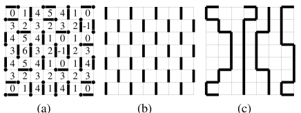
Figure 1: (a) Snapshot of a dimer covering (thick bonds) together with the associated “height” values $h({\bf r})$ for a lattice of size $L=8$ at temperature $T_{d}=1.0$. (b) Dimer covering of the fixed reference. (c) Vortex line configuration (thick lines) obtained as the difference between (a) and (b).

The dimer model is related to the planar vortex-line array via the well-known mapping to the solid-on-solid (SOS) model (see Figs. 1): Define integer heights $\{h\}$ at the centers of squares of ${\cal L}$ which form the dual square lattice ${\cal L}^{D}$, then orient all bonds of ${\cal L}^{D}$ such that elementary squares of ${\cal L}^{D}$ that enclose sites of a chosen sublattice of ${\cal L}$ (solid dots in Fig.1(a)) are circled counterclockwise; Assign $-3$ to the difference of neighboring heights along the oriented bonds if a dimer is crossed and $+1$ otherwise. This yields single-valued heights up to an overall constant. In terms of the height configuration $h({\bf r})$, the partition function (1) can be written alternatively as $Z=\sum_{\{h({\bf r})\}}e^{-\beta{\cal H}[h]}$, where the SOS Hamiltonian takes the following form in the continuum limit,

$$\beta{\cal H}=\int d^{2}{\bf r}\left[\frac{K}{2}(\nabla h)^{2}-{\bf f}({\bf r})\cdot\nabla h+g\cos\left(Gh\right)\right]\;\;.$$ (2)

Here, $K$ is an effective stiffness caused by the inability of a tilted surface to take as much advantage of the low weight bonds as a flatter surface, and ${\bf f}({\bf r})$ is a random local tilt bias. The periodicity of the cosine potential in (2) is given by $G=2\pi/4$ since the smallest “step” of this height profile is four. In the present context of a randomly pinned vortex array, $h({\bf r})$ describes the coarse-grained displacement field of the vortex array with respect to a uniform reference state at the same vortex line density; see Fig. 1(c) and Refs. [5, 8].

The Algorithm:

Computing the partition function of complete dimer coverings on a weighted planar lattice $\cal G$ can be achieved in polynomial time [12]. Weights here refer to the Boltzmann factors $w_{ij}\equiv\exp(-\epsilon_{ij}/T_{d})$ on the bonds. In this article, we shall use the shuffling algorithm by Propp and coworkers[13] to sample the configurational space. The algorithm relates the partition function $Z_{L}$ on a lattice of linear size $L$ to $Z_{L-1}$ as $Z_{L}(\{w\})=C(\{w\})Z_{L-1}(\{w^{\prime}\})$ after a simple weight transformation $\{w\}\rightarrow\{w^{\prime}\}$. The prefactor $C(\{w\})$ is independent of dimer coverings. The partition function is obtained in a “deflation” process in which the above recursive procedure is carried out down to $L=0$ with $Z_{0}=1$. This deflation process can also be reversed in an “inflation” process where a dimer covering at size $L-1$ can be used to stochastically generate a dimer covering at size $L$ according to $Z_{L}$ already obtained. Repeating the inflation process thus generates uncorrelated “importance samplings” of the dimer configurations, or equivalently the equilibrium height configurations, without the need to run the slow relaxational dynamics. The ensuing numerical results are obtained by taking various measurements of the height configurations generated this way. A somewhat inconvenient feature of this approach is that the algorithm requires open boundary condition on the dimer model; this in turn fixes the total number of vortex lines, e.g., to $L/2$ on a $L\times L$ lattice (see Fig. 1).

Numerical results:

Since the temperature of the vortex array, given by $K^{-1}$ in (2), is generally different from the dimer temperature $T_{d}$, we first need to calibrate the temperature scale. To do so, we exploit a statistical rotational symmetry [15, 9] of the system (2) which guarantees that at large scales, the effective $K$ is the same as that of the pure system. In particular, $K$ can be obtained by measuring the disorder-averaged thermal fluctuation of the displacement field $\overline{W_{T}^{2}}\equiv\overline{\langle\prec h_{T}^{2}({\bf r})\succ-\prec h_{T}({\bf r})\succ^{2}\rangle}=(2\pi K)^{-1}\ln(L)$, where $h_{T}({\bf r})\equiv h({\bf r})-\langle h({\bf r})\rangle$ measures the thermal distortion superposed on the distorted “background” $\langle h({\bf r})\rangle$ by the quenched disorder. We used $\prec{...}\succ$, $\langle{...}\rangle$, and overline to denote spatial, thermal, and disorder averages respectively. With the polynomial algorithm, we were able to perform thorough disorder averages for equilibrated systems of sizes up to $512\times 512$. To reduce boundary effects, we focus on the central $L/2\times L/2$ piece of the system and compute its displacement fluctuations. Fig. 2(a) illustrates the dependence of $\overline{W_{T}^{2}}(L)$ for various dimer temperatures $T_{d}$. The linear dependence on $\ln(L)$ is apparent. Identifying the proportionality constant with $(2\pi K)^{-1}$, we obtain the empirical relation between $K^{-1}$ and $T_{d}$ shown in Fig. 2(b). Note that our result recovers the exact relation $K^{-1}(T_{d}\to\infty)=16/\pi$ for the dimer model without disorder [14]. Since the glass transition of the system (2) is expected to occur at temperature $K_{g}^{-1}=4\pi/G^{2}=16/\pi$, our system is glassy for the entire range of dimer temperatures.

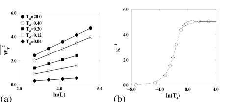
Figure 2: (a) The disorder-averaged thermal displacement fluctuation $\overline{W_{T}^{2}}(L)$ for various dimer temperatures $T_{d}$. Each data point was obtained by generating $10^{3}$ thermal samplings for each of $10^{3}$ disorder realizations. The straight lines are fit to $\overline{W_{T}^{2}}=(2\pi K)^{-1}\ln(L)+{\rm const}$. (b) The extracted relation between $K^{-1}$ and $T_{d}$. The horizontal line indicates the asymptotic value of $K^{-1}$ as $T_{d}\to\infty$.

To probe this glassy state further, we now focus on its magnetic response, i.e., the uniform magnetic susceptibility $\chi$. Due to the constraint of fixed vortex density when using the dimer representation, it is not easy to compute the magnetic susceptibility directly by varying the vortex fugacity (i.e., external magnetic field). Instead, we use the fluctuation-dissipation relation,

$$\chi\propto\lim_{q\rightarrow 0}{\bf q}^{2}\left(\langle\hat{h}_{{\bf q}}\hat{h}_{-{\bf q}}\rangle-\langle\hat{h}_{{\bf q}}\rangle\langle\hat{h}_{-{\bf q}}\rangle\right)\equiv\lim_{q\rightarrow 0}{\bf q}^{2}C_{2}({\bf q}),$$ (3)

where $\hat{h}_{{\bf q}}$ is the Fourier transform of $h({\bf r})$. $\chi$ only probes the system at the largest scale as indicated by the $q\rightarrow 0$ limit, which is evaluated at $(q_{x},q_{y})=(\pi/L,0)$ for finite systems.

As shown in Figs. 3, the distribution $P(\chi)$ at low temperature is peaked at zero and decays more strongly than any power laws for large $\chi$’s. This indicates that the glass phase is typically rigid against the penetration of additional fluxlines when the external magnetic field is increased by a small amount. The mean value $\overline{\chi}$, which takes on a finite value $\propto K^{-1}$ due to the statistical rotational symmetry [9, 15], is however controlled by the rare events contained in the tail of $P(\chi)$. This is similar to the behavior found for a single flux line in $1+1$ dimensional random potential [16, 17].

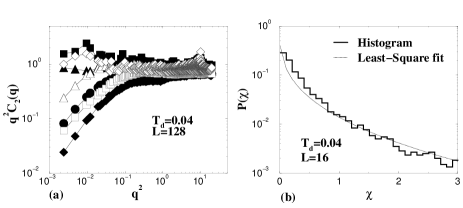
Figure 3: (a) $q^{2}C_{2}({\bf q})$ vs. $q^{2}$. Different symbols denote different disorder realizations, all of which are for $L=128$ at $T_{d}=0.04$. The susceptibility $\chi$ is evaluated at $q=\pi/L$. (b) Probability distribution $P(\chi)$ computed from $6\times 10^{3}$ disorder realizations for $L=16$ at $T_{d}=0.04$. Dotted line is a fit to a stretched exponential $P(\chi)=A\exp(-B\chi^{\alpha})$ with $\alpha=0.5(2)$.

A striking feature of this vortex glass concerns the sample-to-sample variation of the susceptibility $\chi$. It was predicted [9] that the fractional variance,

$${\rm var}[\chi]/\overline{\chi}^{2}\stackrel{{\scriptstyle L\to\infty}}{{\rightarrow}}D|\tau|\qquad{\rm for}\quad 0<-\tau\ll 1,$$ (4)

is universal, with $D$ being a computable, size-independent constant of order unity. Using Eq. (3), we obtain ${\rm var}[\chi]\propto\lim_{{\bf q}\rightarrow 0}{\bf q}^{4}C_{4}({\bf q})$ where $C_{4}({\bf q})\equiv\overline{C_{2}^{2}({\bf q})}-{\overline{C_{2}({\bf q})}}^{2}$. As shown in Fig. 4(a), ${\bf q}^{4}C_{4}({\bf q})$ obeys a power-law scaling as ${\bf q}^{4}C_{4}({\bf q})\sim(qL)^{0.78(2)}$ for small $q$. This behavior is consistent with the analytical prediction that the variance is size-independent because the $q\rightarrow 0$ limit is evaluated at $(q_{x},q_{y})=(\pi/L,0)$ for finite systems. The power-law scaling and its exponent are, however, not understood at present. Finally the temperature dependence of the fractional variance, as shown in Fig. 4(b), can be deduced from the relation between $K^{-1}$ and $T_{d}$ given in Fig. 2(b). It is well described by the linear form (4) close to the glass transition with $D=0.454(5)$.

Figure 4: (a) $q^{4}D({\bf q})$ vs. $(qL)^{2}$ along $q_{y}=0$ axis. Data are obtained by averaging over $10^{3}$ disorder realizations for $L=16,32,64,128,256$ at $T_{d}=0.2$. The solid line is the least square fit; (b) Fractional variance as a function of the reduced temperature, $\tau=1-K_{g}/K$, for $L=32,64,128$, and $256$ averaged over $10^{3}$ disorder realizations. The solid line is a least-square linear fit for $|\tau|<0.15$.

Conclusion.

Finite temperature simulations were performed on a disordered dimer model to study the magnetic response of a planar vortex array. Universal susceptibility variations in the collective pinning regime were observed; critical behavior near the glass transition compared well with analytic predictions. It is hoped that the present study will stimulate further experimental investigations of the physics of mesoscopic vortex systems.

References

- [1] G. Blatter et al, Rev. Mod. Phys. 66, 1125 (1994).
- [2] E. Akkermans et al eds., Mesoscopic Quantum Physics, (North Holland, Amsterdam, 1994).
- [3] C.A. Bolle et al., Nature 399, 43 (1999).
- [4] See, e.g. J.L. Cardy and S. Ostlund, Phys. Rev. B 25, 6899 (1982); J. Toner and D. P. DiVincenzo, Phys. Rev. B 41, 632 (1990);
- [5] M.P. Fisher, Phys. Rev. Lett. 62, 1415 (1989).
- [6] T. Nattermann, I. Lyuksyutov, and M. Schwartz, Europhys. Lett. 16, 295 (1991);
- [7] T. Giamarchi and P. Le Doussal, Phys. Rev. B 52, 1242 (1995).
- [8] T. Hwa, D.R. Nelson, V. M. Vinokur, Phys. Rev. B 67 1167 (1993).
- [9] T. Hwa and D.S. Fisher, Phys. Rev. Lett. 72, 2466 (1994).
- [10] G. G. Batrouni and T. Hwa, Phys. Rev. Lett. 72, 4133 (1994); E. Marinari, R. Monasson, and J. J. Ruiz-Lorenzo, J. Phys. A 28, 3975 (1995); D. Cule and Y. Shapir, Phys. Rev. Lett. 74, 114 (1995);
- [11] L.G. Valiant, Theo. Computer Science 8, 189 (1979).
- [12] P.W. Kasteleyn, Physica 27, 1209 (1961); M.E. Fisher, J. Math. Phys. 7, 1776 (1966).
- [13] N. Elkies, G. Kuperberg, M. Larsen, and J. Propp, J. Algebraic Comb. 1, 111 & 219 (1992); J. Propp, “Urban renewal”, available from http://www-math.mit.edu/propp/articles.html.
- [14] See, e.g., R.W. Youngblood, D.J. Axe, and B.M. McCoy, Phys. Rev. B 21, 5212 (1980); C.L. Henley, J. Stat. Phys. 89, 483 (1997).
- [15] U. Schulz et al, J. Stat. Phys. 51, 1 (1988).
- [16] M. Mezard, J. Phys. (Paris) 51, 1831 (1990).
- [17] T. Hwa and D.S. Fisher, Phys. Rev. B 49, 3136 (1994).