Magnetoresistance of Granular Superconducting Metals in a Strong Magnetic Field

Abstract

The magnetoresistance of a granular superconductor in a strong magnetic field is considered. It is assumed that this field destroys the superconducting gap in each grain, such that all interesting effects considered in the paper are due to superconducting fluctuations. The conductance of the system is assumed to be large, which allows us to neglect all localization effects as well as the Coulomb interaction. It is shown that at low temperatures the superconducting fluctuations reduce the one-particle density of states but do not contribute to transport. As a result, the resistivity of the normal state exceeds the classical resistivity approaching the latter only in the limit of extremely strong magnetic fields, and this leads to a negative magnetoresistance. We present detailed calculations of physical quantities relevant for describing the effect and make a comparison with existing experiments.

I Introduction

In a recent experiment [1], transport properties a system of $Al$ superconducting grains in a strong magnetic field were studied. The samples were quite homogeneous with a typical diameter of the grains $120\pm 20\AA$ and the grains formed a $3$-dimensional array. As usual, sufficiently strong magnetic fields destroyed the superconductivity in the samples and a finite resistivity could be seen above a critical magnetic field. The applied magnetic fields reached $17T$, which was more than sufficient to destroy also the superconducting gap in each grain.

The dependence of the resistivity on the magnetic field observed in Ref.  [1] was not simple. Although at extremely strong fields the resistivity was almost independent of the field, it increased when decreasing the magnetic field. Only at sufficiently weak magnetic fields the resistivity started to decrease and finally the samples displayed superconducting properties. A similar behavior had been reported in a number of publications [2, 3].

A negative magnetoresistance due to weak localization effects is not unusual in disordered metals [4]. However, the magnetoresistance of the granulated materials studied in Ref. [1] is quite noticeable in magnetic fields exceeding $10T$ and is considerably larger than values estimated for the weak localization.

The weak localization effects become very important if the system is near the Anderson metal-insulator transition and one can expect there a complicated dependence on the magnetic field. One can, for example, argue [2] that decreasing the magnetic field drives the system to the metal-insulator transition, which gives a large negative magnetoresistance. If the superconducting transition occurs earlier one gets a maximum of the resistivity near the transition characteristic for the experiments [1, 2, 3].

Unfortunately, investigation of this possibility is not simple. The metal-insulator transition occurs at values of the macroscopic conductance $J$ of the order of unity. At such values calculations are very difficult. The problem becomes even more complicated due to the Coulomb interaction. It is well known [5], that, at small values of $J$, the system must be an insulator even if the superconducting gap is finite in a single grain. A microscopic consideration of all these effects and a confirmation of the existence of the negative magnetoresistance near the superconducting point for $J\sim 1$ is at present hardly possible and we do not try to treat the problem here.

Instead, we consider below the region of large conductances $J\gg 1$, where the system without interactions would be a good metal. This region corresponds to large tunneling amplitudes between the grains. All effects of the weak localization and the charging effects have to be small for $J\gg 1$, which would imply that the resistivity could not considerably depend on the magnetic field.

Nevertheless, we find that the magnetoresistance of a good granulated metal ($J\gg 1$) in a strong magnetic field and at low temperature must be negative. In our model, the superconducting gap in each granule is assumed to be suppressed by the strong magnetic field. All the interesting behavior considered below originates from the superconducting fluctuations that lead to a suppression of the density of states (DOS) but do not help to carry an electric current. The main results have been already published [6] and now we want to present details of calculations and clarify some additional questions. We consider, for example, influence of the Zeeman splitting on the resistivity, find the critical field $H_{C2}$ of the transition into the superconducting state, calculate the diamagnetic susceptibility and estimate weak localization corrections.

Theory of superconducting fluctuations near the transition into the superconducting state has been developed long ago [7, 8, 9] (for a review see Ref. [10]). Above the transition temperature $T_{c}$, non-equilibrium Cooper pairs are formed and a new channel of charge transfer opens (Aslamazov-Larkin contribution)[7]. Another fluctuation contribution comes from a coherent scattering of the electrons forming a Cooper pair on impurities (Maki-Thompson contribution)[8]. Both the fluctuation corrections increase the conductivity and, when a magnetic field is applied, lead to a positive magnetoresistance. Formation of the non-equilibrium Cooper pairs results also in a fluctuational gap in the one-electron spectrum [9] but in conventional (non granular) superconductors the first two mechanisms are more important near $T_{c}$ and the conductivity increases when approaching the transition. The total conductivity for a bulk sample above the transition temperature $T_{c}$ can be written in the following form

$$\sigma=\sigma_{Drude}+\delta\sigma,$$ (1)

where $\sigma_{Drude}=(e^{2}\tau n)/m$ is the conductivity of a normal metal without electron-electron interaction, $\tau$ is the elastic mean free time, $m$ and $n$ are the effective mass and the density of electrons, respectively. In Eq. (1), $\delta\sigma$ is a correction to the conductivity due to the fluctuations of the virtual cooper pairs

$$\delta\sigma=\delta\sigma_{DOS}+\delta\sigma_{AL}+\delta\sigma_{MT}$$ (2)

where $\delta\sigma_{DOS}$ is the correction to the conductivity due to the reduction of the DOS and $\delta\sigma_{AL}$ and $\delta\sigma_{MT}$ stand for the Aslamazov-Larkin (AL) and Maki-Thompson (MT) contributions the conductivity. Close to the critical temperature $T_{c}$ the AL correction is more important than both the MT and DOS corrections types and its contribution can be written as follows [7]

$$\frac{\delta\sigma_{AL}}{\sigma_{Drude}}=\lambda\left(\frac{T_{c}}{T-T_{c}}\right)^{\beta}$$ (3)

where $\lambda$ is a small dimensionless positive parameter $\lambda\ll 1$ and $\beta=1/2$ for the three-dimensional case (3D), 1 for 2D and 3/2 for quasi-1D. Eq. (3) was derived using a perturbation theory and therefore is valid provided the inequality $\delta\sigma_{AL}/\sigma_{Drude}\ll 1$ is fulfilled.

Although typically the AL and MT corrections are larger than the DOS contribution, a small decrease of the transverse conductivity is possible in layered materials [11] in a temperature interval not very close to the transition. It is relevant to emphasize that all previous study of the fluctuations has been done near the critical temperature $T_{c}$ in a zero or a weak magnetic field. In contrast, we are mainly concentrated on study of the transport at very low temperature in a strong magnetic field. To the best of our knowledge, fluctuations in this region have not been considered so far.

A strong magnetic field destroys the superconducting gap in each granule. However, even at magnetic fields $H$ exceeding the critical field $H_{c}$ virtual Cooper pairs can still be formed. It turns out, and it will be shown below, the influence of these pairs on the macroscopical transport is drastically different from that near $T_{c}$. The existence of the virtual pairs leads to a reduction of the DOS but, in the limit $T\rightarrow 0,$ these pairs cannot travel from one granule to another. As a result, the conductivity $\sigma$ can be at $H>H_{c}$ considerably lower than conductivity $\sigma_{0}$ of the normal metal without an electron-electron interaction. It approaches the value $\sigma_{0}$ only in the limit $H\gg H_{c},$ when all the superconducting fluctuations are completely suppressed by the magnetic field.

The superconducting pairing inside the grains is destroyed by both the orbital mechanism and the Zeeman spliting. The critical magnetic field $H_{c}^{or}$ destroying the superconductivity in a single grain in this case can be estimated as $H_{c}^{or}R\xi\approx\phi_{0}$, where $\phi_{0}=hc/e$ is a flux quantum, $R$ is a radius of single grain and $\xi=\sqrt{\xi_{0}l}$ is the superconducting coherence length. The Zeeman critical magnetic field $H_{c}^{z}$ can be written as $g\mu_{B}H_{c}^{z}=\Delta_{0}$, where $\Delta_{0}$ is a BCS gap for the single grain at magnetic field $H=0$ and $g$ is a Lande factor. We notice here that $H_{c}^{z}$ is independent of the size of the grain whereas for $H_{c}^{or}$ the size of the grain is important. The ratio of this two fields can be written in the form

$$H_{c}^{or}/H_{c}^{z}\approx R_{c}/R,$$ (4)

where $R_{c}=\xi(p_{0}l)^{-1}$. We can see from Eq. (4) that for $R>R_{c}$ the orbital critical magnetic field is smaller than the Zeeman critical magnetic field $H_{c}^{or}<H_{c}^{z}$ and the suppression of superconductivity is due to the orbital mechanism. This condition is well satisfied in grains with $R\sim 100\AA$ studied in [1]. This limit is opposite to the one considered recently in Ref. [12] where the Zeeman splitting was assumed to be the main mechanism of destruction of the Cooper pairs. However, the latter mechanism of the destruction of the Cooper pairs can be easily included into the scheme of our calculations.

The remainder of the paper is organized as follows. In Sec. II we formulate the model and discuss the fluctuational contributions to the total conductivity of the granulated superconductors. Sec.  III contains the derivation of the correction to the conductivity of granulated superconductors due to single electron tunnelling (DOS contribution) at very low temperatures $T\ll T_{c}$ and strong magnetic fields $H-H_{c}\ll H_{c}$. In Sec.  IV and Sec. V corrections to the conductivity due to tunneling of virtual Cooper pairs are derived (Aslamazov-Larkin and Maki-Thompson corrections). In Sec. VI we discuss the influence of magnetic field on the phase of order parameter and calculate the critical field of the transition into the superconducting phase. The importance of the Zeeman splitting is discussed in Sec. VII. The contribution of fluctuating Cooper pairs to the diamagnetic susceptibility of granular system is derived in Sec.VIII. Sec. IX includes the results for conductivity at $T-T_{c}\ll T_{c}$ and $H\ll H_{c}$. A discussion of a recent experiment in $Al$ grains and a comparison with the theory is presented in Sec. X Our results are summarized in the Conclusion.

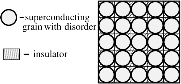
FIG. 1.: System of metallic grains

II Choice of the model

We consider a 3D array of superconducting grains coupled to each other, Fig. 1. The grains are not perfect and there can be impurities inside the grains as well as on the surface. We assume that electrons can hop from grain to grain and can interact with phonons.

The Hamiltonian $\hat{H}$ of the system can be written as

$$\hat{H}=\hat{H}_{0}+\hat{H}_{T},$$ (5)

where $\hat{H}_{0}$ is a conventional Hamiltonian for a single grain with an electron-phonon interaction in the presence of a strong magnetic field

$$\hat{H}_{0}=\sum\limits_{i,k}E_{i,k}a_{i,k}^{{\dagger}}a_{i,k}-|\lambda|\sum\limits_{i,k,k^{\prime}}a_{i,k}^{{\dagger}}a_{i,-k}^{{\dagger}}a_{i,-k^{\prime}}a_{i,k^{\prime}}+\hat{H}_{imp},$$ (6)

where $i$ stands for the numbers of the grains, $k\equiv({\bf k},\uparrow)$, $-k\equiv(-{\bf k},\downarrow)$; $\lambda$ is an interaction constant, and $\hat{H}_{imp}$ describes elastic interaction of the electrons with impurities. The interaction in Eq. (6) contains diagonal matrix elements only. This form of the interaction can be used provided the superconducting gap $\Delta_{0}$ is not very large

$$\Delta_{0}\ll E_{c}$$ (7)

where $E_{c}$ is the Thouless energy of the single granule. Eq. (7) is equivalent to the condition $R\ll\xi_{0}$, where $R$ is the radius of the grain and $\xi_{0}$ is the superconducting coherence length. In this limit, superconducting fluctuations in a single grain are zero-dimensional.

The term $\hat{H}_{T}$ in Eq.(5) describes tunneling from grain to grain and has the form (see e.g. Ref. [14])

$$\hat{H}_{T}=\sum\limits_{i,j,p,q}t_{ijpq}a_{ip}^{{\dagger}}a_{jq}\exp(i\frac{e}{c}{\bf A}{\bf d}_{ij})+h.c.$$ (8)

where ${\bf A}$ is the external vector potential; ${\bf d}_{ij}$ are the vectors connecting centers of two neighboring grains $i$ and $j$ ($\left|{\bf d}_{ij}\right|=2R$); $a_{ip}^{{\dagger}}\left(a_{ip}\right)$ are the creation (annihilation) operators for an electron the grain $i$ and state $p$.

It is assumed that the system is macroscopically a good metal and this corresponds to a sufficiently large tunneling energy $t$

$$t\gg\delta$$ (9)

where $\delta=\left(\nu_{0}V\right)^{-1}$ is the mean level spacing in a single granule, $\nu_{0}=mp_{0}/2\pi^{2}$ is the DOS per one spin in the absence of interactions, $V$ is the volume of the granule, and $\Delta_{0}$ is the Bardeen-Cooper-Schrieffer (BCS) gap at $T=0$ in the absence of a magnetic field. Provided the inequality (9) is fulfilled localization effects can be neglected Ref. [13]. Moreover, charging effects are also not important in this limit because at such tunneling energies the Coulomb interaction is well screened.

The tunneling current operator is

$$\hat{{\bf j}}=-ie{\bf d}\sum\limits_{j,p,q}t_{ijpq}a_{ip}^{{\dagger}}a_{jq}\exp(i\frac{e}{c}{\bf A}{\bf d}_{ij})-h.c.$$ (10)

Using standard formulae of the linear response theory we can write the current ${\bf j}\left(t\right)$ in the form

$${\bf j}(t)=i\int\limits_{-\infty}^{t}\langle[{\bf\hat{\jmath}}(t),{\bf\hat{\jmath}}(t^{\prime})]\rangle{\bf A}(t^{\prime})dt^{\prime}-ie^{2}{\bf d}^{2}\int\limits_{-\infty}^{t}\langle[\hat{H}_{T}(t),\hat{H}_{T}(t^{\prime})]\rangle dt^{\prime}{\bf A}(t),$$ (11)

where the angle brackets stand for averaging over both quantum states and impurities in the grains. All operators in the right hand side of Eq. (11) are independent of the vector potential. In principle, the grains can be clean and the electrons can scatter mainly on the surface of the grains. However, provided the shape of the grains corresponds to a classically chaotic motion of the electrons, the clean limit should be described in the $0D$ case by the same formulae.

We carry out the calculation of the conductivity making expansion both in fluctuation modes and in the tunneling term $H_{T}$. This implies that the tunneling energy $t$ is not very large. Proper conditions will be written later but now we mention only that the tunneling energy $t$ will be everywhere much smaller than the energy $E_{c}$.

As in conventional bulk superconductors we can write corrections to the classical conductivity as a sum of corrections to the DOS and of Aslamazov-Larkin (AL) $\sigma_{AL}$ and Maki-Thompson (MT) $\sigma_{MT}$ corrections. Diagrams describing these contributions are represented in Fig. 2.

FIG. 2.: Diagram a) describes correction to DOS, diagrams b) and c) describe corrections to conductivity due to superconducting fluctuations. The wavy lines denote the propagator of the fluctuations, the dashed lines stand for the impurity scattering.

The total conductivity $\sigma$ can be written as

$$\sigma=\sigma_{DOS}+\sigma_{AL}+\sigma_{MT}$$ (12)

where $\sigma_{DOS}$ is given by equation

$$\sigma_{DOS}=\sigma_{0}\left(4T\right)^{-1}\int\limits_{-\infty}^{+\infty}[\nu(\varepsilon)/\nu_{0}]^{2}\cosh^{-2}(\frac{\varepsilon}{2T})d\varepsilon,$$ (13)

In Eq. (13), $\sigma_{0}=2\pi e^{2}R^{-1}\left(t/\delta\right)^{2}$ is the classical conductivity of the granular metal. It can be rewritten in terms of the dimensionless conductance of the system $J$ as

$$\sigma_{0}=\frac{8Je^{2}}{\pi R}$$ (14)

where the conductance $J$ equals

$$J\equiv(\pi^{2}/4)(t/\delta)^{2}$$ (15)

The inequality (9) is equivalent to the condition

$$J\gg 1$$ (16)

The function $\nu\left(\varepsilon\right)$ in Eq. (13) is the density of states. Without the electron-electron interaction, this function is equal to the DOS of the ideal electron gas $\nu_{0}$, which gives $\sigma_{DOS}=\sigma_{0}$. Taking into account the electron-electron attraction we can write the contribution $\sigma_{DOS}$ to the classical conductivity as

$$\sigma_{DOS}=\sigma_{0}+\delta\sigma_{DOS}(t,T,H)$$ (17)

The correction $\delta\sigma_{DOS}\left(t,T,H\right)$ depends on temperature $T$ and magnetic field $H$ and is represented in Fig. 2a. As concerns the long range part of the Coulomb interaction (charging effects), the condition $J\gg 1$ allows us to neglect it.

Using Eq. (13) the correction to the conductivity $\delta\sigma_{DOS}$ at low temperatures can be written in terms of the correction to the DOS at zero energy $\delta\nu\left(0\right)$ as

$$\delta\sigma_{DOS}/\sigma_{0}=2(\delta\nu\left(0\right)/\nu_{0})$$ (18)

As we will see below, the main contribution to the conductivity due to the superconducting fluctuations comes from the change of the DOS $\delta\nu$. Its calculation will be presented in detail in the next Section.

III
Suppression of the conductivity due to DOS fluctuations

In this Section we consider the correction to the conductivity of granulated superconductors due to suppression of DOS. The main correction $\delta\nu\left(\varepsilon\right)$ to the DOS of the non-interacting electrons $\nu_{0}$ is described by the diagram in the Fig. 2a, while the terms $\ \sigma_{MT}$ and $\sigma_{AL}$ are given by Figs. 2b and 2c, respectively. The calculation of the diagrams can be performed for the Matsubara frequencies $\varepsilon_{n}=\pi T(2n+1)$ using temperature Green functions. At the end one should, as usual Ref. [15], make the analytical continuation $i\varepsilon_{n}\rightarrow\varepsilon$ . The magnetic field will be considered in the quasi-classical approximation $l\ll L_{c}$, where $l$ is a mean free path and $L_{c}$ is a cyclotron radius. In this approximation, the magnetic field results in the appearance of additional phases in Green functions

$$G(i\epsilon_{n},\vec{r},\vec{r^{\prime}})=G^{(0)}(i\epsilon_{n},\vec{r}-\vec{r^{\prime}})\exp\left(\frac{ie}{c}\int\limits_{\vec{r}}^{\vec{r^{\prime}}}\vec{A}d\vec{r}\right),$$ (19)

where $G^{(0)}(i\epsilon_{n},\vec{r}-\vec{r^{\prime}})$ is the Green function without magnetic field. In the zero order approximation in the superconducting fluctuations, the disorder averaged Green function $G^{(0)}$ in the momentum representation has the form:

$$G^{\left(0\right)}\left(i\varepsilon_{n},{\bf p}\right)=\left(i\varepsilon_{n}-\xi\left({\bf p}\right)+i\left(2\tau\right)^{-1}sgn\varepsilon_{n}\right)^{-1}$$ (20)

The diagrams in Fig. 2 contain the averaged one-particle Green functions, the impurity vertices proportional to the so called Cooperon $C$ and the propagator of the superconducting fluctuations $K$. The functions $C$ and $K$ depend on the coordinates and time slower than the averaged one-particle Green functions because the characteristic scale for both the impurity vertices and the propagator of superconducting fluctuations $K$ is the coherence length $\xi$ which is much larger than $l$. As a result, the magnetic field affects only the vertex $C$ and the propagator $K$, whereas the phases of the Green functions drawn in Fig.2 outside these blocks cancel. So, reading the diagrams in Fig.1 one should replace the solid lines by the functions $G^{\left(0\right)}\left(i\varepsilon_{n},{\bf p}\right)$. More complicated diagrams containing crossings of impurity lines describe the weak localization effects are neglected here.

The impurity vertex entering these diagrams is equal to $\left(2\pi\nu_{0}\tau\right)^{-1}C\left(i\varepsilon_{n},i\Omega_{k}-i\varepsilon_{n}\right)$, Fig. 3, where $\tau$ is the mean free time due to the scattering on impurities or on the grain boundary, $C$ is the Cooperon. It obeys the following equation

$$\left(D_{0}\left(-i{\bf\nabla-}\left(2e/c\right){\bf A}\right)^{2}+|2\varepsilon_{n}-\Omega_{k}|\right)C\left({\bf r,r}^{\prime}\right)=2\pi\nu_{0}\delta\left({\bf r-r}^{\prime}\right)$$ (21)

where $D_{0}=v_{0}^{2}\tau/3$ is the classical diffusion coefficient. The vector-potential ${\bf A}\left({\bf r}\right)$ should be chosen in the London gauge. If the shape of the grain is close to spherical, the vector-potential is expressed through the magnetic field ${\bf H}$ as ${\bf A}\left({\bf r}\right)=[{\bf H\times r]/}2$.

FIG. 3.: Impurity vertex.

All relevant energies in the problem are assumed to be much smaller than the energy of the first harmonics $E_{c}=D_{0}\pi^{2}/R^{2}$ playing the role of the Thouless energy of a single grain and this allows to keep only the zero harmonics in the spectral expansion of the solution $C\left({\bf r,r}^{\prime}\right)$ of Eq. (21). One can find the eigenvalue ${\cal E}_{0}\left(H\right)$ of this harmonics using the first order of the standard perturbation theory

$${\cal E}_{0}\left(H\right)=\left(2e/c\right)^{2}D_{0}<{\bf A}^{2}>_{0}$$ (22)

where $<...>_{0}$ stands for the averaging over the volume of the grain. For the grain of a nearly spherical form one obtains

$${\cal E}_{0}\left(H\right)=\frac{2}{5}\left(\frac{eHR}{c}\right)^{2}D_{0}=\frac{2}{5}\left(\frac{\phi}{\pi\phi_{0}}\right)^{2}E_{c}$$ (23)

where $\phi_{0}=\pi c/e$ is the flux quantum and $\phi$ is the magnetic flux through the granule.

Within the zero-harmonics approximation, the function $C$ does not depend on coordinates and equals

$$C\left(i\varepsilon_{n},i\Omega_{k}-i\varepsilon_{n}\right)=2\pi\nu_{0}\left(|2\varepsilon_{n}-\Omega_{k}|+{\cal E}_{0}\left(H\right)\right)^{-1}$$ (24)

To calculate the propagator of the superconducting fluctuations $K$ one should sum the sequence of the ladder diagrams represented in Fig. 4. The broken lines in this figure denote the electron-electron interaction. As it has been mentioned the characteristic energies of the propagator $K$ are low and therefore, when calculating the function $K$, one should take into account the tunneling processes from grain to grains. The tunneling Hamiltonian $H_{T}$, Eq. (8), is represented in Fig. 4 by crossed circles.

FIG. 4.: Propagator of superconducting fluctuations with tunneling.

Of course, one can sum the ladder diagrams in Fig.4 directly. However, sometimes it is more convenient to decouple the electron-electron interaction in Eq. (6) by a Gaussian integration over an auxiliary field $\Delta$ (Hubbard-Stratonovich transformation). Then, one can perform averaging over the electron quantum states, thus reducing the calculation to computation of a functional integral over the field $\Delta$. In principle, one obtains within such a scheme a complicated free energy functional and the integral cannot be calculated exactly. The situation simplifies if the fluctuations are not very strong. Then, one can expand the free energy functional in $\Delta$ and come to Gaussian integrals that can be treated without difficulties. For the problem considered the propagator $K$ is proportional to the average of the square of the field $\langle{|\Delta_{k}|}^{2}\rangle$. In terms of the functional integral this quantity is written as

$$\langle{|\Delta|}^{2}\rangle=\frac{\int{|\Delta|}^{2}\exp(-\beta F_{eff}[\Delta,\Delta^{\ast}])D\Delta D\Delta^{\ast}}{\int\exp(-\beta F_{eff}[\Delta,\Delta^{\ast}])D\Delta D\Delta^{\ast}}$$ (25)

here $\beta=1/T$ and $F_{eff}[\Delta,\Delta^{\ast}]$ is the effective free energy functional. We have chosen the parameters in such a way that the grains are zero-dimensional. Therefore, it is sufficient to integrate over the zero space harmonics only, which means that the field $\Delta$ in the integral in Eq. (25) does not depend on coordinates. In the quadratic approximation in the field $\Delta$ the free energy functional $F_{eff}$ includes two different terms

$$F_{eff}=F_{eff}^{(1)}+F_{eff}^{(2)}$$ (26)

where $F_{eff}^{(1)}$ describes the superconducting fluctuations in an isolated grain and $F_{eff}^{(2)}$ takes into account tunneling from grain to grain. For the first term we obtain after standard manipulations

$$F_{eff}^{(1)}\left[\Delta,\Delta^{\ast}\right]=V\sum_{\Omega_{k}}\left(1/\left|\lambda\right|-T\sum_{2\varepsilon_{n}>\left|\Omega_{k}\right|}2C\left(i\varepsilon_{n}\right)\right){|\Delta(\Omega_{k})|}^{2}$$ (27)

where the function $C(i\varepsilon_{n})$ is defined in Eq.(24) and $V$ is the volume of a single grain. In the limit of low temperatures $T\ll{\cal E}_{0}(H)$ the sum over the frequencies $\varepsilon_{n}$ in Eq. (27) can be replaced by the integral and we reduce the functional $F_{eff}^{(1)}\left[\Delta,\Delta^{\ast}\right]$ to the form

$$F_{eff}^{(1)}\left[\Delta,\Delta^{\ast}\right]=\frac{1}{\delta}\sum_{\Omega_{k}}\left(\ln\left(\frac{{\cal E}_{0}(H)+|\Omega_{k}|}{\Delta_{0}}\right)\right){|\Delta(\Omega_{k})|}^{2}$$ (28)

Close to the critical magnetic field $H_{c}$ destroying the superconducting gap in a single grain the energy of the first harmonics ${\cal E}_{0}(H)$ is equal to the BSC gap at zero temperature $\Delta_{0}$. This means that Eq. (28) can be written in this case in the region $T\ll\Delta_{0}$. Near $H_{c}$ small frequencies $\Omega_{k}$ are most important and one can expand Eq. (28) in powers of the small parameter $\Omega_{k}/\Delta_{0}$. Then, we obtain

$$F_{eff}^{(1)}\left[\Delta,\Delta^{\ast}\right]=\frac{1}{\delta}\sum_{\Omega_{k}}\left(\ln\left(\frac{{\cal E}_{0}(H)}{\Delta_{0}}\right)+\frac{|\Omega_{k}|}{\Delta_{0}}\right){|\Delta(\Omega_{k})|}^{2}$$ (29)

At strong magnetic fields $H\gg H_{c}$, one should use the more general formula, Eq. (28).

The term $F_{eff}^{(2)}\left[\Delta,\Delta^{\ast}\right]$ describing the tunneling includes three different contributions represented in Fig. 5

FIG. 5.: Diagrams describing $F_{eff}^{(2)}$.

The analytical expression $F_{eff}^{(21)}\left[\Delta,\Delta^{\ast}\right]$ corresponding to the first diagram Fig. 5 can be written as

$$F_{eff}^{(21)}\left[\Delta,\Delta^{\ast}\right]=-t^{2}/(2\pi\nu_{0}\tau)^{2}\sum_{i,j}(\Delta_{i}\Delta_{j}^{\ast}+c.c.)V^{2}\int\frac{d^{3}{\bf p}_{i}d^{3}{\bf p}_{j}}{{(2\pi)}^{6}}T\sum_{\varepsilon_{n}}G(i\varepsilon_{n}{\bf p}_{i})G(-i\varepsilon_{n}{\bf p}_{i})G(i\varepsilon_{n}{\bf p}_{j})G(-i\varepsilon_{n}{\bf p}_{j})C^{2}(i\varepsilon_{n})$$ (30)

Writing Eq. (30) we put $\Omega_{k}=0$ in the expression for the Cooperon $C$ and in the Green functions. This is justified because the energy $F_{eff}^{\left(2\right)}\left[\Delta,\Delta^{\ast}\right]$ is already small because it includes the parameter $J(\delta/{\cal E}_{0}(H))$ that is assumed to be small, where $J$ is the dimensionless conductance of the system specified by Eq. (15). Next terms of the expansion are of the order of $J(\delta/{\cal E}_{0}(H))(\Omega_{k}/{\cal E}_{0}(H))$ and can be neglected for small $\Omega_{k}$. The second and third diagrams in Fig. 5 are equal to each other and have the opposite sign with respect to the first diagram. For simplicity we assume that the granules are packed into a cubic lattice. Using the momentum representation with respect to the coordinates of the grains and taking into account all diagrams in Fig. 5 we reduce the free energy functional $F_{eff}^{\left(2\right)}\left[\Delta,\Delta^{\ast}\right]$ to the form

$$F_{eff}^{(2)}\left[\Delta,\Delta^{\ast}\right]=(8/3\pi)(1/\delta)\sum_{i=1}^{3}J(\delta/{\cal E}_{0}(H))\left(1-\cos q_{i}d\right){|\Delta|}^{2}$$ (31)

where ${\bf q}$ is the quasi-momentum and $d=2R$. Eq. (31) is written in the limit

$$J\ll{\cal E}_{0}(H)/\delta$$ (32)

The inequality (32) is compatible with the inequality (16) provided the inequality

$${\cal E}_{0}(H)\gg\delta$$ (33)

is fulfilled. If ${\cal E}_{0}(H)\sim\Delta_{0}$, the condition, Eq. (33), is at the same time the condition for the existence of the superconducting gap in the single granule. The inequality (32) allows us also to neglect influence of the tunneling on the form of the Cooperon, so we use for calculations Eq. (24).

Writing the previous equations for $F_{eff}^{(2)}\left[\Delta,\Delta^{\ast}\right]$ we neglected the influence of magnetic field on the phase of the order parameter $\Delta$. In other words we omitted the phase factor $\exp(i\frac{e}{c}\int{\bf A}({\bf r})d{\bf r})$. The effect of the magnetic field on the phase will be discussed in details later in Sec. VI.

Although the final result for the correction to the DOS can be written for arbitrary temperatures $T$ and magnetic fields $H$, let us concentrate on the most interesting case $T\ll T_{c}$, $H>H_{c}$. Using Eqs. (25,28,31) we obtain for the propagator of the superconducting fluctuations $K\left(i\Omega_{k,}{\bf q}\right)$

$\displaystyle K(i\Omega_{k},{\bf q})=-\nu_{0}^{-1}\left(\ln\left(\frac{{\cal E}_{0}(H)+\left|\Omega_{k}\right|}{\Delta_{0}}\right)+\eta({\bf q})\right)^{-1},$

$$\eta({\bf q})\equiv\left(8/3\pi\right)\sum_{i=1}^{3}J\left(\delta/{\cal E}_{0}(H)\right)\left(1-\cos q_{i}d\right),$$ (34)

The pole of the propagator $K(i\Omega_{k},{\bf q})$ at ${\bf q}=0$, $\Omega_{k}=0$ determines the field $H_{c}$, at which the BCS gap disappears in a single grain. From the form of Eq. (34) we find

$${\cal E}_{0}(H_{c})=\Delta_{0}.$$ (35)

The result for $H_{c}$, Eqs. (23, 35), agrees with the one obtained long ago by another method [16]. We can see from Eqs. (34, 35) that the term $\eta({\bf q})$ describing tunneling is very important if $H$ is close to $H_{c}$.

Eqs. (24), (34) give the explicit formulae for the functions $C$ and $K$ and allow us to calculate the correction $\delta\nu$ to the DOS . The analytical expression for the diagram, Fig. 2a, reads as follows

$$\delta\nu(i\varepsilon_{n})=(1/\pi)1/{(2\pi\nu_{0}\tau)}^{2}\int\frac{d^{3}{\bf q}}{{(2\pi)}^{3}}T\sum_{\Omega_{k}}K(i\Omega_{k},{\bf q})\int\frac{d^{3}{\bf p}}{{2\pi}^{3}}C^{2}(i\varepsilon_{n},i\Omega_{k}-i\varepsilon_{n})G^{2}(i\varepsilon_{n},{\bf p})G(i\Omega_{k}-i\varepsilon_{n},{\bf p})$$ (36)

Eq. (36) contains integration over the momentum in the single grain ${\bf p}$ and the quasi-momentum ${\bf q}$. First, we integrate over the momentum ${\bf p}$ and reduce Eq. (36) for $\varepsilon_{n}>0$ to the form

$$\delta\nu(i\varepsilon_{n})=\frac{2iT}{\nu_{0}}\sum\limits_{\Omega_{k}<\varepsilon_{n}}\int K(i\Omega_{k},{\bf q})C^{2}\left(i\varepsilon_{n},i\Omega_{k}-i\varepsilon_{n}\right)\frac{d^{3}{\bf q}}{\left(2\pi\right)^{5}}$$ (37)

After calculation of the sum over $\Omega_{k}$ in Eq. (37), one should make the analytical continuation $i\varepsilon_{n}\rightarrow\varepsilon$. At low temperatures, it is sufficient to find the correction to the DOS at zero energy $\delta\nu\equiv\delta\nu\left(0\right)$.

Remarkably, Eqs. (34-37) do not contain explicitly the mean free time $\tau$. This is a consequence of the zero-harmonics approximation, which is equivalent to using the random matrix theory (RMT) Ref. [13]. (The parameter $\tau$ enters only Eq. (23) giving the standard combination ${\cal E}_{0}\left(H\right)$ describing in RMT the crossover from the orthogonal to the unitary ensemble). This justifies the claim that the results can be used also for clean grains with a shape providing a chaotic electron motion.

Using Eqs. (13, 34-37) one can easily obtain an explicit expression for $\sigma_{DOS}$ for $H-H_{c}\ll H_{c}$. In this limit, one expands the logarithm in the denominator of Eq.(34) and neglects the dependence of $C$ on $\varepsilon_{n}$ and $\Omega_{k}$ because the main contribution in the sum over $\Omega_{k}$ comes from $\Omega_{k}\sim{\cal E}_{0}(H)-{\cal E}_{0}(H_{c})\ll\Delta_{0}$. Using Eq. (18) the result for $\delta\sigma_{DOS}=\sigma_{0}-\sigma_{DOS}$ can be written as

$$\frac{\delta\sigma_{DOS}}{\sigma_{0}}=-\frac{2\delta}{\Delta_{0}}\left\{\begin{array}[]{lr}-\pi^{-1}<\ln\tilde{\eta}\left({\bf q}\right)>_{q},&T/\Delta_{0}\ll\tilde{\eta}\\ \frac{2T}{\Delta_{0}}<\tilde{\eta}^{-1}({\bf q})>_{q},&\tilde{\eta}\ll T/\Delta_{0}\ll 1\end{array}\right.,$$ (38)

$\displaystyle\tilde{\eta}({\bf q})=\eta({\bf q})+2h,\quad<...>_{q}\equiv V\int\limits_{0}^{2\pi/d}\left(...\right)d{\bf q/}\left(2\pi\right)^{3}$where $h=\left(H-H_{c}\right)/H_{c}$ and $V$ is a volume of the single grain. We see that the correction to the conductivity is negative and its absolute value decreases when the magnetic field increases. The correction reaches its maximum at $H\rightarrow H_{c}$. At zero temperature and close to the critical field $H_{c}$ such that $J(\delta/\Delta_{0})\gg h$, the maximum value of $\delta\sigma_{DOS}/\sigma_{0}$ from Eq. (38) is

$$\left|\frac{\delta\sigma_{DOS}}{\sigma_{0}}\right|=\frac{2}{\pi}\frac{\delta}{\Delta_{0}}\left\langle\ln\left(\frac{1}{\eta({\bf q})}\right)\right\rangle_{q}=\frac{1}{3}\frac{\delta}{\Delta_{0}}\ln\left(\frac{\Delta_{0}}{J\delta}\right).$$ (39)

In the limit $J(\delta/\Delta_{0})\ll h\lesssim 1$, one can expand the logarithm in Eq. (38). Then, taking $h\sim 1$ the correction to the conductivity at zero temperature can be estimated as

$$\left|\frac{\delta\sigma_{DOS}}{\sigma_{0}}\right|\sim J\left(\frac{\delta}{\Delta_{0}}\right)^{2}$$ (40)

Schematically, the suppression of the DOS due to the superconducting fluctuations is shown in Fig. 6.

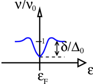
FIG. 6.: Suppression of DOS due to superconducting fluctuations.

As temperature grows, the correction to the conductivity due to the reduction of the DOS can become larger and reach for $T\sim\Delta_{0}$ and $J(\delta/\Delta_{0})\gg h$ the order of magnitude of $J^{-1}$.

$$\frac{|\delta\sigma_{DOS}|}{\sigma_{0}}=4(\delta T/\Delta_{0}^{2})\left\langle\frac{1}{h+\eta({\bf q})}\right\rangle_{q}\sim\frac{1}{J}$$ (41)

In the limit $h\approx 1\gg J(\delta/\Delta_{0})$ and at temperature $T\sim\Delta_{0}$ this correction can be estimated as

$$\frac{\delta\sigma_{DOS}}{\sigma_{0}}\approx\frac{\delta}{\Delta_{0}}$$ (42)

We see from Eqs. (39-42) that the corrections to the conductivity are smaller than unity provided we work in the regime of a good metal, Eqs. (9, 16), so the diagrammatic expansion we use is justified. Indeed, we can neglect the corrections of higher orders. For example, the diagram shown in Fig. 7 has the additional small factor of $(\delta/\Delta_{0})\ln\tilde{\eta}$ at $T/\Delta_{0}\ll\tilde{\eta}$ and $\delta/(\Delta_{0}\tilde{\eta})$ at $\tilde{\eta}\ll T/\Delta_{0}$.

FIG. 7.: An example of high order corrections to DOS.

The correction to the conductivity calculated in this Section could become comparable with $\sigma_{0}$ when $J\sim 1$. However, such values of $J$ mean that we would be in this case not far from the metal-insulator transition. Then, we would have to take into account all localization effects. For values of $J\sim 1$ one can use Eq. (38) for rough estimates only. Apparently, the parameters of the samples of Ref. [1] correspond to the region $J\sim 1$, $\delta/\Delta_{0}\sim 1/3$.

In the limit of strong magnetic fields $H\gg H_{c}$ the correction to $\sigma_{0}$ can still be noticeable. In this case we can use Eq. (28) as before but, with a logarithmic accuracy, we can neglect the dependence of the superconducting propagator, Eq.(34), on $\Omega_{k}$ and on the tunneling term. Then we obtain finally

$$\delta\sigma_{DOS}/\sigma_{0}=-(1/3)\left(\delta/{\cal E}_{0}(H)\right)\ln^{-1}\left({\cal E}_{0}(H)/\Delta_{0}\right)$$ (43)

Eq. (43) shows that in the region $H\gg H_{c}$ the correction to the conductivity decays essentially as $\delta\sigma_{DOS}\sim H^{-2}$.

Let us emphasize that the correction to the conductivity coming from the DOS remains finite in the limit $T\rightarrow 0$, thus indicating the existence of the virtual Cooper pairs even at $T=0$.

In the region of not very small $h\gg J\delta/\Delta_{0}$, we can neglect the tunneling term $F_{eff}^{\left(2\right)}\left[\Delta,\Delta^{\ast}\right]$ in the free energy functional $F_{eff}\left[\Delta,\Delta^{\ast}\right]$. Then, we can write the correction to the conductivity in a rather general form. The superconducting propagator $K$ can be written in this case as

$$K(i\Omega_{k})=-\nu_{0}^{-1}\ln^{-1}\left(\frac{{\cal E}_{0}(H)+|\Omega_{k}|}{\Delta_{0}}\right)$$ (44)

Using Eq. (37) for the correction to the DOS and Eq. (18) we obtain for the correction to the conductivity at zero temperature

$$\frac{\delta\sigma_{DOS}}{\sigma_{0}}=-\frac{1}{3}\left(\frac{\delta}{\Delta_{0}}\right)\int\limits_{a}^{\infty}\frac{\exp{(-x)}}{x}dx=-\frac{1}{3}\left(\frac{\delta}{\Delta_{0}}\right)Ei(a),\hskip 28.45274pta=2\ln(1+h)$$ (45)

In the limit $h\ll 1$, we reproduce with logarithmic accuracy Eq. (39), whereas in the opposite limiting case $h\gg 1$ we come to Eq. (43).

In order to calculate the entire conductivity, Eq. (12), we must investigate the AL and MT contributions (Figs. 2c and 2b). In conventional superconductors near $T_{c}$, these contributions are most important leading to an increase of the conductivity. In the granular materials, the situation is much more interesting. It turns out that both the AL and MT contributions vanish in the limit $T\rightarrow 0$ at all $H>H_{c}$ and thus, the correction to the conductivity comes from the DOS only. So, at low temperatures, estimating the total correction to the classical conductivity $\sigma_{0}$, Eq. (14), one can use the formulae of this Section.

IV Aslamasov-Larkin correction to the conductivity

The Aslamasov-Larkin (AL) correction to the conductivity $\sigma_{AL}$ originates from the ability of virtual Cooper to carry an electrical current. In contrast to the one-electron tunneling determining $\sigma_{DOS}$, the probability of tunneling of the Cooper pairs from one grain to another is proportional to $t^{4}$. The quantity $\sigma_{AL}$ is related to the response function $Q^{AL}$ as

$\displaystyle\sigma_{AL}=Q^{AL}/(-i\omega),\omega\rightarrow 0$where the diagram for the $Q^{AL}(i\omega_{n})$ is represented in Fig. 2c. Calculating integrals corresponding to this diagram we may put $\Omega_{k}=0$ in the electron loops, because all singularities in the vicinity of the transition point are contained in the propagator of the superconducting fluctuations $K(i\Omega_{k})$ [7]. The analytical expression for the diagram in Fig. 2c has the form

$$Q^{AL}(i\omega_{n})=4/3\sum_{i=1}^{3}\int\frac{d^{3}{\bf q}}{{(2\pi)}^{3}}T\sum_{\Omega_{k}}K(i\Omega_{k},{\bf q})K(i\Omega_{k}-i\omega_{n},{\bf q})B_{1}^{2}(0,{\bf q})$$ (46)

where $B_{1}(0,{\bf q})$ corresponds to one electron loop. The analytical expression for this loop reads

$$B_{1}(0,{\bf q})=- 4i\int\sin q_{i}^{\prime}d\cos(q_{i}-q_{i}^{\prime})d\frac{d^{3}{\bf q}^{\prime}}{{(2\pi)}^{3}}\frac{edt^{2}V^{2}}{{(2\pi\nu_{0}\tau)}^{2}}\times$$ (48)

$$\int\frac{d^{3}{\bf p}_{1}d^{3}{\bf p}_{2}}{{(2\pi)}^{6}}T\sum_{\varepsilon_{n}}G(i\varepsilon_{n},{\bf p}_{1})G(-i\varepsilon_{n},{\bf p}_{1})G(i\varepsilon_{n},{\bf p}_{2})G(-i\varepsilon_{n},{\bf p}_{2})C^{2}(i\varepsilon_{n})$$

The functions $\sin q^{\prime}_{i}d$ and $\cos(q_{i}-q^{\prime}_{i})d$ in Eq. (48) correspond to the current and tunneling vertices, respectively. Eq. (46) is obtained by considering four different types of AL diagrams that are obtained from each other by permutations of the current and tunneling vertices. Summing over the spin of the electrons we get the additional factor $2$. As in the preceding Section we calculate the impurity vertices neglecting the tunneling term, which is justified if the inequality (32) is fulfilled. Integrating over the momenta ${\bf p}_{1}$ and ${\bf p}_{2}$ in Eq. (48) we reduce the functions $B_{1}(0,{\bf q})$ to the following form

$$B_{1}(0,{\bf q})=-\frac{8}{\pi^{2}}J\frac{ed}{{\cal E}_{0}(H)}4i\int\sin q_{i}d\cos(q_{i}-q_{i}^{\prime})d\frac{d^{3}{\bf q}^{\prime}}{{(2\pi)}^{3}}$$ (49)

To calculate the response function $Q^{AL}$ for real frequencies $\omega$ one has to make an analytical continuation from the Matsubara frequencies $\omega_{n}$. This can be done rewriting the sum over $\Omega_{k}$ in Eq. (46) in a form of a contour integral that allows to make the continuation $i\omega_{n}\rightarrow\omega+i0$. As a result, we obtain [7]

$$T\sum_{\Omega_{k}} K\left(i\Omega_{k},{\bf q}\right)K\left(i\Omega_{k}-i\omega_{n},{\bf q}\right)\rightarrow$$ (51)

$$\frac{1}{4\pi i}\left(\int_{-\infty}^{+\infty}\coth\frac{\varepsilon}{2T}(K^{R}(\varepsilon)-K^{A}(\varepsilon))K^{A}(\varepsilon-\omega)d\varepsilon+\int_{-\infty}^{+\infty}\coth\frac{\varepsilon}{2T}(K^{R}(\varepsilon)-K^{A}(\varepsilon))K^{R}(\varepsilon+\omega)d\varepsilon\right)$$

where $K^{R}(K^{A})$ is retarded (advanced) superconducting fluctuation propagator. Expanding Eq. (51) in $\omega$ we keep the term that remains finite in the limit $\omega\rightarrow 0$ and the linear one. The zero order term cancels with the contribution of a diagram schematically represented in Fig.2c but containing instead of the current vertices the tunneling ones. The latter contribution originates from the second term in Eq. (11). The linear term giving the dc conductivity can be written as

$$T\sum_{\Omega_{k}}K\left(i\Omega_{k},{\bf q}\right)K\left(i\Omega_{k}-i\omega_{n},{\bf q}\right)\rightarrow-i\frac{2\omega{\cal E}_{0}^{2}(H)}{\pi\nu_{0}^{2}}\int_{0}^{+\infty}\coth\frac{\varepsilon}{2T}\frac{\varepsilon({\varepsilon}^{2}-{\eta}^{2})}{{({\eta}^{2}+{\varepsilon}^{2})}^{3}}d\varepsilon$$ (52)

where $\eta({\bf q})$ is defined in Eq. (34). Using Eqs. (46, 49,52) the fluctuational contribution $\sigma_{AL}$ to the conductivity is reduced in the limit $T\ll T_{c}$, $H-H_{c}\ll H_{c}$ to the form

$$\frac{\sigma_{AL}}{\sigma_{0}}=\frac{16}{9}J\frac{\delta^{2}T}{\Delta_{0}^{3}}\sum\limits_{i=1}^{3}<A\left({\bf q}\right)[{\tilde{\eta}({\bf q})]}^{-3}{\ \sin}^{2}q_{i}d>_{q}$$ (53)

where $A\left({\bf q}\right)=4\pi T\left(3\Delta_{0}\tilde{\eta}({\bf q})\right)^{-1}$ for $T\ll\Delta_{0}\tilde{\eta}$ and $A\left({\bf q}\right)=1$ for $\Delta_{0}\tilde{\eta}\ll T<T_{c}$.

Using Eq. (53) we can estimate the quantity $\sigma_{AL}/\sigma_{0}$.

Let us consider first the limit $T\ll\Delta_{0}\tilde{\eta}$. In this region, provided the inequality $h\ll J\delta/\Delta_{0}$ is fulfilled, the main contribution in Eq. (53) comes from small $q$. Calculating the integral over ${\bf q}$ we obtain from Eq. (53)

$$\frac{\sigma_{AL}}{\sigma_{0}}=\frac{32\pi^{2}}{71}J\frac{\delta^{2}T^{2}}{{\Delta_{0}}^{4}}\int_{0}^{\infty}\frac{x^{2}d^{3}x}{\left(h+J(\delta/\Delta_{0})x^{2}\right)^{4}}\sim J^{-3/2}\frac{T^{2}}{\Delta_{0}^{3/2}\delta^{1/2}}\left(\frac{H_{c}}{H-H_{c}}\right)^{3/2}$$ (54)

From Eq. (54) we can see that at low temperatures the AL correction to the conductivity is proportional to the square of the temperature  $\sigma_{AL}\sim T^{2}$ and vanishes in the limit $T\rightarrow 0$.

Let us compare the AL correction with correction due to suppression of the DOS considered in the previous Section. Using Eqs. (54) and (39) we obtain

$$\frac{\sigma_{AL}}{|\delta\sigma_{DOS}|}\sim J^{-3/2}\frac{T^{2}}{\Delta_{0}^{1/2}\delta^{3/2}}\ln^{-1}\left(\frac{\Delta_{0}}{J\delta}\right)\left(\frac{H_{c}}{H-H_{c}}\right)^{3/2}.$$ (55)

We see from Eq. (55) that at $T\ll\Delta_{0}\tilde{\eta}$ the AL correction is small $|\sigma_{AL}/\delta\sigma_{DOS}|\ll 1$. This means that the AL contribution cannot change the monotonous increase of the resistivity of granulated superconductors when decreasing the magnetic field. At very strong magnetic fields $H\gg H_{c}$, we can neglect the second term in the denominator of Eq. (54). Then the AL correction can be estimated as

$$\frac{\sigma_{AL}}{\sigma_{0}}\sim J\frac{\delta^{2}T^{2}}{\Delta_{0}^{4}}\left(\frac{H_{c}}{H}\right)^{4}$$ (56)

To compare this result with the correction due to the DOS we should use Eq. (43) that was also derived at strong magnetic field $H\gg H_{c}$.

$$\left|\frac{\sigma_{AL}}{\delta\sigma_{DOS}}\right|\sim J\frac{\delta T^{2}{\cal E}_{0}(H)}{\Delta_{0}^{4}}\left(\frac{H_{c}}{H}\right)^{4}\ln\left(\frac{{\cal E}_{0}(H)}{\Delta_{0}}\right)$$ (57)

Using Eq. (23) for ${\cal E}_{0}(H)$ we can see from Eq. (57) that $|\sigma_{AL}/\delta\sigma_{DOS}|_{H\gg H_{c}}\sim H^{-2}$.

Now let us consider the region of temperatures not far from the critical temperature $\Delta_{0}\tilde{\eta}\ll T\leq T_{c}$. Using Eq. (53) we have

$$\frac{\sigma_{AL}}{\sigma_{0}}=\frac{8\pi}{27}J\frac{\delta^{2}T}{\Delta_{0}^{3}}\int\frac{Vd^{3}q\sin^{2}qd}{\left(h+J(\delta/\Delta_{0})(1-\cos qd)\right)^{3}}$$ (58)

In the limit $J(\delta/\Delta_{0})\gg h$, the main contribution in Eq. (58) comes from small $q$ and the contribution $\sigma_{AL}$ can be written as

$$\frac{\sigma_{AL}}{\sigma_{0}}=\frac{8\pi}{27}J(\delta^{2}/{\Delta_{0}}^{2})\int\frac{x^{2}d^{3}x}{\left(h+J(\delta/\Delta_{0})x^{2}\right)^{3}}\sim J^{-3/2}\left(\frac{\Delta_{0}}{\delta}\right)^{1/2}\left(\frac{H_{c}}{H-H_{c}}\right)^{1/2}$$ (59)

We see that the AL contribution grows when approaching the critical field $H_{c}$. In order to calculate the AL correction we used the perturbation theory. Therefore, the region of the validity of the results obtained is described by the inequalities $\sigma_{AL}/\sigma_{0}\ll 1$ or $h\gg J^{-3}(\Delta_{0}/\delta)$.

Now let us compare the AL correction with $\delta\sigma_{DOS}$. From Eqs. (58, 41) we obtain

$$\frac{\sigma_{AL}}{|\delta\sigma_{DOS}|}\sim J^{-1/2}\left(\frac{\Delta_{0}}{\delta}\right)^{1/2}\left(\frac{H_{c}}{H-H_{c}}\right)^{1/2}.$$ (60)

Eq. (60) is correct only at fields close to the critical field, such that the inequality $h\ll J^{-1}(\Delta_{0}/\delta)$ is fulfilled. In this region the total correction to the conductivity is positive, which means the resistivity decays, when approaching the critical magnetic field $H_{c}$. In the case of a strong magnetic field $H\gg H_{c}$, we can neglect the second term in the denominator of Eq. (58) and then we obtain

$$\frac{\sigma_{AL}}{\sigma_{0}}\sim J\left(\frac{\delta}{\Delta_{0}}\right)^{2}\left(\frac{H_{c}}{H}\right)^{3}$$ (61)

that is $\sigma_{AL}\sim H^{-3}$ at $H\gg H_{c}$ and $T\sim\Delta_{0}$.

To understand the behavior of the total conductivity of the granulated superconductors in this region we should consider also the Maki-Thompson contribution and this will be done in the next Section.

V Maki-Thompson correction to the conductivity

Another contribution usually increasing the conductivity is the Maki-Thompson (MT) contribution represented in Fig. 2b. Again, we can put $\Omega_{k}=0$ in the electron loop, because characteristic frequencies in superconducting fluctuation propagator $K$ are of the order $\Omega_{k}\sim\Delta_{0}\tilde{\eta}\ll{\cal E}_{0}$. The analytical expression for this diagram reads

$$Q^{MT}(i\omega_{n})=2/3\sum_{i=1}^{3}\int\frac{d^{3}{\bf q}}{{(2\pi)}^{3}}T\sum_{\Omega_{k}}K(i\Omega_{k},{\bf q})B_{2}(i\omega_{n},{\bf q})$$ (62)

where $B_{2}(i\omega_{n},{\bf q})$ is a function describing the contribution of the loop. This function can be written as follows

$$B_{2}(i\omega_{n},{\bf q})=4\int\sin q_{i}^{\prime}d\sin(q_{i}-q_{i}^{\prime})d\frac{d^{3}{\bf q}^{\prime}}{{(2\pi)}^{3}}\frac{e^{2}d^{2}t^{2}V^{2}}{{(2\pi\nu_{0}\tau)}^{2}}\times$$ (63)

$$\int\frac{d^{3}{\bf p}_{1}d^{3}{\bf p}_{2}}{{(2\pi)}^{6}}T\sum_{\varepsilon_{n}}G(-i\varepsilon_{n},{\bf p}_{1})G(i\varepsilon_{n},{\bf p}_{1})G(-i\varepsilon_{n}+i\omega_{n},{\bf p}_{1})G(i\varepsilon_{n}-i\omega_{n},{\bf p}_{2})C(i\varepsilon_{n})C(-i\varepsilon_{n}+i\omega_{n},i\varepsilon_{n}-i\omega_{n})$$ (64)

where, as before, ${\bf p}_{1}$ and ${\bf p}_{2}$ stand for the momenta in the granules and ${\bf q}$, ${\bf q}^{\prime}$ are quasi-momenta. Eq. (62) includes the contribution of two different MT diagrams and summation over spins. In order to make the analytical continuation $i\omega_{n}\rightarrow\omega+i0$ in Eqs. (62), (64) it is convenient to rewrite the sum over $\varepsilon_{n}$ in the form of the following contour integral

$$T\sum_{\varepsilon_{n}}...=\frac{1}{4\pi i}( \int_{C_{1}} \tanh\frac{z}{2T}G^{A}(-z,{\bf p}_{1})G^{R}(z,{\bf p}_{1})G^{A}(-z+i\omega_{n},{\bf p}_{2})G^{R}(z-i\omega_{n},{\bf p}_{2})C^{R}(z)C^{R}(z-i\omega_{n})dz+$$ (65)

$$\int_{C_{2}} \tanh\frac{z}{2T}G^{A}(-z,{\bf p}_{1})G^{R}(z,{\bf p}_{1})G^{R}(-z+i\omega_{n},{\bf p_{2}})G^{A}(z-i\omega_{n},{\bf p_{2}})C^{R}(z)C^{A}(z-i\omega_{n})dz+$$ (66)

$$\int_{C_{3}} \tanh\frac{z}{2T}G^{R}(-z,{\bf p}_{1})G^{A}(z,{\bf p_{1}})G^{R}(-z+i\omega_{n},{\bf p}_{2})G^{A}(z-i\omega_{n},{\bf p}_{2})C^{A}(z)C^{A}(z-i\omega_{n})dz),$$ (67)

where the contours $C_{1},C_{2},C_{3}$ are shown in Fig. 8.

FIG. 8.: Contour of integration.

As usual, the MT diagrams have both regular (contours $C_{1},C_{3}$) and anomalous (contour $C_{2}$) part. Near $T_{c}$ and at very low magnetic field the anomalous part can be very large. In the limit $H\rightarrow 0$, it can even diverge and become larger that the AL correction giving a positive contribution to the conductivity [10]. However, in the limit of high magnetic fields and $T\rightarrow 0$, the situation is less intriguing. It turns out that for the problem considered, the absolute values of the regular and anomalous parts are equal in this limit but these contributions have the opposite signs. Making the analytical continuation in Eq. (67) and integrating over the momenta we obtain in the lowest order in $\omega$

$$\frac{1}{4\pi i}\left(\int_{C_{1}}+\int_{C_{2}}+\int_{C_{3}}\right)\rightarrow\frac{8\pi i\omega}{{\delta}^{2}}\int_{0}^{+\infty}\tanh\frac{\varepsilon}{4T}\frac{\varepsilon({\cal E}_{0}^{2}-{\varepsilon}^{2})}{({\cal E}_{0}^{2}{+{\varepsilon}^{2}})^{3}}d\varepsilon$$ (68)

where the energy ${\cal E}_{0}={\cal E}_{0}\left(H\right)$ is given by Eq. (23). From Eq. (68), we see that at $T=0$ the MT contribution vanishes, which corresponds to the cancelation of the regular and anomalous parts. At low but finite temperatures $T$, the final result for the MT contribution can be written as

$$\frac{\sigma_{MT}}{\sigma_{0}}=\frac{16{\pi}^{2}T^{2}\delta}{9\Delta_{0}^{3}}\sum\limits_{i=1}^{3}<B\left({\bf q}\right)\cos q_{i}d>_{q}$$ (69)

where $B\left({\bf q}\right)=$ $-\pi^{-1}\ln\tilde{\eta}({\bf q})$ for $T\ll\Delta_{0}\tilde{\eta}$ and $B\left({\bf q}\right)=2T\left(\Delta_{0}\tilde{\eta}({\bf q})\right)^{-1}$ for $\Delta_{0}\tilde{\eta}\ll T\lesssim T_{c}$

Let us estimate the MT contribution in the different limiting cases. At low temperatures $T\ll\Delta_{0}\tilde{\eta}$ and $h\ll J\delta/\Delta_{0}$ we have from Eq. (69)

$$\frac{\sigma_{MT}}{\sigma_{0}}=\frac{16\pi}{9}\frac{T^{2}\delta}{\Delta_{0}^{3}}\left\langle\ln\left(\frac{1}{h+J(\delta/\Delta_{0})(1-\cos q)}\right)\cos q\right\rangle_{q}\sim\frac{T^{2}\delta}{\Delta_{0}^{3}}$$ (70)

Comparing Eq. (70) with Eq. (39) we come to the following estimate

$$\frac{\sigma_{MT}}{|\delta\sigma_{DOS}|}\sim\left(\frac{T}{\Delta_{0}}\right)^{2}\ln^{-1}\left(\frac{\Delta_{0}}{J\delta}\right)$$ (71)

If the magnetic field $H$ is not very close to $H_{c}$, such that $J\delta/\Delta_{0}\ll h\lesssim 1$, we obtain from Eq. (69)

$$\frac{\sigma_{MT}}{|\delta\sigma_{DOS}|}\sim\left(\frac{T}{\Delta_{0}}\right)^{2}$$ (72)

We can see from Eqs. (71, 72) that the MT contribution $\sigma_{MT}$ is proportional at low temperatures to $T^{2}$, which is the same temperature dependence as that for the AL contribution. This means that, at sufficiently low temperatures, the MT contribution is small, $\sigma_{MT}/\delta\sigma_{DOS}\ll 1$. Thus, we conclude that, in this region, the main correction to the classical conductivity, Eq. (14) comes from the correction to the DOS, Eq. (39). The latter correction is negative, so the resistivity of the granulated superconductors exceeds its classical value.

It is interesting to compare the AL and MT corrections.  In the limit $T\rightarrow 0$, and $h\ll J\delta/\Delta_{0}$, we obtain using Eqs. (54) and (70)

$$\frac{\sigma_{MT}}{\sigma_{AL}}\approx\left(J\frac{\delta}{\Delta_{0}}\right)^{3/2}\left(\frac{H-H_{c}}{H_{c}}\right)^{3/2}$$ (73)

Eq. (73) shows that in this region, The AL contribution is larger the MT one. Let us consider another case of not very low temperatures, $\Delta_{0}\tilde{\eta}\ll T\leq T_{c}$. From Eq. (69) we have

$$\frac{\sigma_{MT}}{\sigma_{0}}=\frac{16\pi^{3}}{27}\frac{T^{2}\delta}{\Delta_{0}^{3}}\int\frac{Td^{3}x\cos x}{\Delta_{0}\left(h+J(\delta/\Delta_{0})(1-\cos x)\right)}\sim\frac{1}{J}$$ (74)

Eq. (74) gives the possibility to compare the MT contribution with the DOS in this temperature interval. Recalling Eq. (41) we obtain

$$\frac{\sigma_{MT}}{|\delta\sigma_{DOS}|}\sim 1$$ (75)

Eq. (75) shows that at not very low temperatures the MT contribution has the same order of magnitude as the contribution due to the reduction of the DOS. At the same time, the AL contribution in the region $\Delta_{0}\tilde{\eta}\ll T\lesssim T_{c}$ can be considerably larger than both the MT and DOS contributions.

From Eqs. (59) and (74) we can see that at $T\lesssim T_{c}$

$$\frac{\sigma_{MT}}{\sigma_{AL}}\approx J^{1/2}\left(\frac{\delta}{\Delta_{0}}\right)^{1/2}\left(\frac{H-H_{c}}{H_{c}}\right)^{1/2}.$$ (76)

Eqs. (75,76) show that, at not very low temperatures, and not far from the critical field the AL correction to the conductivity is the most important. This means that approaching the transition in this region the resistivity decreases, which is in contrast to the behavior at very low temperature where the correction to the resistivity is determined entirely by the contribution to the DOS and is positive.

To conclude the last two Sections we emphasize once more that the temperature and magnetic field dependence of $\sigma_{AL}$ and $\sigma_{MT}$ is rather complicated but they are definitely positive. The competition between these corrections and $\sigma_{DOS}$ determines the sign of the magnetoresistance. We see from Eqs. (53, 69) that both the AL and MT contributions are proportional at low temperatures to $T^{2}$. Therefore the $\sigma_{DOS}$ in this limit is larger and the magnetoresistance is negative for all $H_{c}$. In contrast, at $T\sim T_{c}$ and close to $H_{c}$, the AL and MT corrections can become than $\sigma_{DOS}$ resulting in a positive magnetoresistance in this region. Far from $H_{c}$ the magnetoresistance is negative again.

VI The critical field $H_{c_{2}}$ in the granulated superconductors

In the previous Sections we considered transport in granulated superconductors at magnetic fields $H$ not far from the field $H_{c}$. The field $H_{c}$ is the field destroying the superconducting gap in a single isolated granule. We have seen that the main contribution due to the superconducting fluctuations comes from the correction to the density of states, Eq. (38), and this correction remains finite in the limit $H\rightarrow H_{c}$. But is the field $H_{c}$ a critical field in the system of the granules coupled to each other by tunneling? If it were a critical field what would happen at $H<H_{c}$? Would the system be macroscopically the superconductor or normal metal? Or, may be, this would be a new state of matter?

To answer these questions we should derive the effective action $F_{eff}\left[\Delta,\Delta^{\ast}\right]$, Eqs. (26, 28, 31), more carefully than it has been done in Sec.III. Namely, until now we considered only the effect of the magnetic field on the electron motion inside the grains, neglecting its influence on the correlation of the phases of the order parameter $\Delta_{i}$ of different grains. However, to understand whether the system is macroscopically superconductor or not, we must consider the macroscopic motion and thus, the effect of the magnetic field on the phase correlation.

In this Section we come back to the derivation of effective action $F_{eff}\left[\Delta,\Delta^{\ast}\right]$ taking into account the influence of magnetic field on the phases of the order parameter. First, we consider this problem qualitatively and then, quantitatively. It is clear that if the magnetic field is strong enough, it induces macroscopic currents that finally, at a field $H_{c_{2}}$, destroy the superconductivity.

Let us estimate the critical magnetic field $H_{c_{2}}$ using the Ginzburg-Landau theory. We assume that the granulated system under consideration is in the macroscopically superconducting state. Then, the Josephson part of the free energy in the coordinate representation, not too close to the $H_{c_{2}}$, can be written in the form

$$F=\sum\limits_{i}E_{J}\frac{(\Delta_{i}-\Delta_{j})^{2}}{\Delta_{0}^{2}}\approx\int d^{3}{\bf r}\frac{(\nabla\Delta)^{2}}{R\Delta_{0}^{2}}E_{J}$$ (77)

where $E_{J}=J\Delta_{0}$ is the Josephson energy, $J\gg 1$ is the dimensionless conductance, Eq. (15), $\Delta_{0}$ is the BCS gap at zero magnetic field and $R$ is a radius of the single grain. The gradient expansion in Eq. (77) was done under the assumption that the magnetic flux through one grain is smaller than the flux quantum $\phi_{0}$.

In the conventional Ginzburg-Landau free energy the coefficient in front of the gradient term is proportional to the square of the coherence length $\xi$. Therefore, using Eq. (77) we can extract the macroscopic coherence length $\xi$. Recalling that the free energy of a single grain is $\nu V\Delta^{2}$, where $V$ is a volume of single grain, we obtain

$$\xi^{2}\sim JR^{2}(\delta/\Delta_{0})$$ (78)

If the conductance $J$ is large enough the behavior of the granulated superconductors is the same as in a bulk sample with the effective coherence length $\xi$. Now we estimate the critical magnetic field $H_{c_{2}}$ that destroys the superconductivity in the system as $H_{c_{2}}\xi^{2}\approx\phi_{0}$. This field is different from the field $H_{c}$. Using Eq. (35) we can compare these two fields. The result for the ratio of these two fields is

$$\frac{H_{c}}{H_{c_{2}}}\approx J\frac{\delta}{\Delta_{0}}\sqrt{\frac{R}{\xi_{0}}}$$ (79)

Eq. (79) for $H_{c_{2}}$ is valid provided $H_{c_{2}}\ll H_{c}$, which corresponds to the inequality $J\gg(\Delta_{0}/\delta)\sqrt{\xi_{0}/R}$. However, we are interested in the opposite case when

$$1\ll J\ll(\Delta_{0}/\delta)\sqrt{\xi_{0}/R}$$ (80)

This contradict to the assumption made and means that, in the region specified by Eq. (80), the critical field $H_{c_{2}}$ is close to the field $H_{c}$ and $\left|H_{c}-H_{c_{2}}\right|/H_{c}$ can be considered as a small parameter.

Now let us calculate the critical magnetic field $H_{c_{2}}$ more rigorously taking into account the influence of the magnetic field on the macroscopic motion. The magnetic field results in an additional phase factor $\exp(i\frac{e}{c}\int{\bf A(r)}d{\bf r})$ in the superconducting field $\Delta_{i}$ in Eq. (30). We assume that this magnetic field is not far from $H_{c}$ determined by Eqs. (23, 35). The field $H_{c}$ is of order $\phi_{0}/R\xi$, which means that, in the limit under consideration $R\ll\xi$, the magnetic flux through the elementary cell of the lattice of the granules is small. Therefore, we can expand the functions $\exp(i\frac{e}{c}\int{\bf A(r)}d{\bf r})$ in ${\bf A}$ and write gradients instead of the finite differences of $\Delta_{i}$ in Eq. (30). Essential frequencies $\Omega_{k}$ are also small and the free energy functional in such a continuum approximation takes the form

$$F\left[\Delta,\Delta^{\ast}\right]=\frac{1}{\delta}\sum\limits_{\Omega_{k}}\left(\ln\left(\frac{{\cal E}_{0}(H)}{\Delta_{0}}\right)+\frac{\mid\Omega_{k}\mid}{{\cal E}_{0}(H)}+\frac{4d^{2}}{3\pi}J\left(\frac{\delta}{{\cal E}_{0}(H)}\right)\left(\nabla-\frac{2ie}{c}{\bf A}\right)^{2}\right)\left|\Delta\right|^{2}$$ (81)

The critical magnetic field $H_{c_{2}}$ can be found writing the propagator of the superconducting fluctuation $K$ corresponding to the free energy, Eq. (81). Making Fourier transformation of the function $\Delta$ in the eigenfunctions of the operator entering Eq. (81) and calculating Gaussian integrals we obtain for the propagator $K_{n}\left(0,q_{z}\right)$ in the spectral representation at $\Omega_{k}=0$

$$K_{n}(0,q_{z})=-\nu_{0}^{-1}\left(\ln\left(\frac{{\cal E}_{0}(H)}{\Delta_{0}}\right)+\frac{4d^{2}}{3\pi}J\left(\frac{\delta}{{\cal E}_{0}(H)}\right)\left(q_{z}^{2}+4(n+1/2)\frac{H}{\phi_{0}}\right)\right)^{-1}$$ (82)

where $q_{z}$ is a component of the quasi-momentum parallel to the magnetic field and $n=0,1...$ are the number of the Landau levels. To calculate the critical magnetic field $H_{c_{2}}$ we should consider poles of the superconducting propagator. Taking the lowest Landau number $n=0$ and putting $q_{z}=0$ obtain the following equation determining the critical field $H_{c_{2}}$

$$\ln\left(\frac{{\cal E}_{0}(H_{c_{2}})}{\Delta_{0}}\right)+\frac{8d^{2}}{3\pi}J\left(\frac{\delta}{\Delta_{0}}\right)\frac{H_{c}}{\phi_{0}}=0$$ (83)

Expanding the first term in Eq. (83) near $H_{c}$ we find the critical field $H_{c_{2}}$

$$H_{c_{2}}=H_{c}\left(1-\frac{40}{\pi^{2}}J\left(\frac{\delta}{\Delta_{0}}\right)\sqrt{\frac{R^{2}}{\xi_{0}l}}\right)$$ (84)

Eq. (84) shows us that the critical field $H_{c_{2}}$ is close to the field $H_{c}$ so long as $\left(J\delta/\Delta_{0}\right)\left(R/\xi\right)\ll 1,$ where $\xi\sim\left(\xi_{0}l\right)^{1/2}$ is the coherence length in the superconducting grains. Eq. (32) and the assumption that the grains are zero-dimensional guarantee the fulfillment of this inequality. For the ballistic motion of  electrons inside the grain (the radius of the grain $R$ is of the order of the mean free path, $R\sim l$) the critical field $H_{c_{2}}$ can be written in the form

$$\frac{H_{c}-H_{c_{2}}}{H_{c}}=\frac{40}{\pi^{2}}J\left(\frac{\delta}{\Delta_{0}}\right)\sqrt{\frac{R}{\xi_{0}}}\ll 1$$ (85)

Eq. (84) is the main result of this Section. Below the magnetic field $H_{c_{2}}$, one should add in Eq. (81) a term quartic in $\Delta$, which gives a non-zero order parameter $\Delta.$ Thus, at field $H<H_{c_{2}}$ the granular system is in the superconducting state.

In order to understand the behavior of the resistivity as a function of the magnetic field $H$ in the region $H_{c_{2}}<H<H_{c}$ we can consider the quantity $\frac{\partial}{\partial H}\left(\frac{\delta\sigma}{\sigma_{0}}\right)$. We can use as before Eq. (37) but now, calculating the integral, we should make the following replacement

$\displaystyle\int\left(...\right)\frac{d^{3}{\bf q}}{\left(2\pi\right)^{3}}\rightarrow\frac{H}{\phi_{0}}\int\sum\limits_{n=0}^{\infty}(...)\frac{dq_{z}}{2\pi}$where $q_{z}$ is a component of the quasi-momentum parallel to the magnetic field.

The correction to the DOS at $T=0$ takes the form

$$\delta\nu(0)=\frac{1}{2\pi^{2}\nu_{0}}C^{2}T\sum\limits_{\Omega_{k}<0}\left(\frac{H}{\phi_{0}}\right)\sum\limits_{n=0}^{\infty}\int K_{n}(i\Omega_{k},q_{z})\frac{dq_{z}}{(2\pi)}$$ (86)

The main contribution to the correction $\delta\nu(0)$ in Eq. (86) comes from the term with $n=0$. Using the fact that $\delta\sigma/\sigma_{0}=2\delta\nu/\nu_{0},$ taking the first derivative with respect to the magnetic field and finally, integrating over the frequency $\Omega$ and quasi-momentum $q_{z}$ we obtain

$$\frac{\partial}{\partial H}\left(\frac{\delta\sigma}{\sigma_{0}}\right)=-15\sqrt{\frac{\pi}{24}}\frac{1}{H_{c}}\left(\frac{\delta}{J\Delta_{0}}\right)^{1/2}\left(\frac{R^{2}}{\xi_{0}l}\right)^{1/2}\left(\frac{H_{c_{2}}}{H-H_{c_{2}}}\right)^{1/2},$$ (87)

where $H_{c_{2}}$ is given by Eq. (84). We can see from Eq. (87) that the value $\frac{\partial}{\partial H}\left(\frac{\delta\sigma}{\sigma_{0}}\right)$ diverges when $H$ approaches $H_{c_{2}}$. Thus, the critical field $H_{c_{2}}$ is characterized by the infinite slope on the dependence of the resistivity on the magnetic field. This property might help to identify this field on experimental curves.

VII Zeeman splitting.

In our previous consideration we neglected interaction between the magnetic field and spins of the electrons. This approximation is justified if the size of the grains is not very small. Then, the critical field $H_{c}^{or\text{ }}$destroying the superconducting gap is smaller than the paramagnetic limit $g\mu H_{c}^{Z}=\Delta_{0}$ and the orbital mechanism dominates the magnetic field effect on the superconductivity. However, the Zeeman splitting leading to the destruction of the superconducting pairs can become important if one further decreases the size of the grains.

Let us discuss now the effect of Zeeman splitting. We can rewrite Eq. (4) for the ratio of orbital $H_{c}^{or}$ magnetic field to the Zeeman magnetic field in the following form

$$\frac{H_{c}^{or}}{H_{c}^{Z}}=\left(\frac{\delta}{\delta_{c}}\right)^{1/3}$$ (88)

where $\delta_{c}\approx 1/(\nu R_{c}^{3})$, $R_{c}=\xi(p_{0}l)^{-1}$ and $\xi=\sqrt{\xi_{0}l}$. To understand whether the Zeeman splitting is important for an experiment we can estimate the ratio $\delta_{c}/\Delta_{0}$ and compare it with the proper experimental result. We find easily

$$\frac{\delta_{c}}{\Delta_{0}}=(p_{0}l)\sqrt{\frac{l}{\xi_{0}}}$$ (89)

which shows $\delta_{c}/\Delta_{0}$ can be both smaller than $(\delta/\Delta_{0})_{exper.}$ and larger depending on the values of $l$ and $\xi_{0}$. Using the result for $\delta_{c}$, Eq. (89), we can rewrite Eq. (88) as

$$\frac{H_{c}^{or}}{H_{c}^{Z}}=\left(\frac{\delta}{\Delta_{0}}\frac{R}{l}\right)^{1/2}$$ (90)

In the experiment [1], both the mechanisms are in principle important. One can come to this conclusion using the fact that the Zeeman critical magnetic field is $H_{c}^{Z}\approx 3.5T$ and this is not far from the peak in the resistivity at the field $H\approx 2.5T$. Below, we consider the corrections to the DOS and conductivity due to the Zeeman mechanism. We will see that at temperature $T=0$ these corrections can be of the same order of magnitude as the correction due to orbital mechanism.

Let us calculate first the critical magnetic field $H_{0}$ destroying the superconducting gap in a single grain taking into account both the orbital and Zeeman mechanisms of the destruction. The Green function for the non-interacting electrons in this case is

$$G_{\uparrow\downarrow}^{(0)}(i\varepsilon_{n},{\bf p})=\frac{1}{i\varepsilon_{n}-\xi({\bf p})\pm E_{Z}/2+(i/2\tau)sgn(\varepsilon_{n})},$$ (91)

where $E_{Z}=g\mu_{B}H$ is the Zeeman energy. Including the interaction between the magnetic field and electron spins we obtain the following form of the Cooperon

$$C(i\varepsilon_{n},-i\varepsilon_{n})=2\pi\nu_{0}(\left|2\varepsilon_{n}\right|-iE_{Z}sgn\left(\varepsilon_{n}\right)+{\cal E}_{0}(H))^{-1}$$ (92)

Repeating the calculations of Sec. III with the modified Cooperon, Eq. (92), we find at $T\ll Tc$   the new critical magnetic field $H_{0}$

$${\cal E}_{0}^{2}(H_{0})+E_{Z}^{2}(H_{0})=\Delta_{0}^{2}$$ (93)

In the limit of a very week Zeeman splitting, when the orbital mechanism is more important, Eq. (93) reproduces the previous result for the critical magnetic field Eq. (35). In the opposite limiting case, when the Zeeman mechanism plays the major role, we obtain $E_{Z}=\Delta_{0}$. In general case, when the both mechanisms of the destruction of the conductivity are important, one should solve Eq. (93) and the result reads

$$H_{0}=H_{c}\left(-\frac{1}{2}\left(\frac{g\mu_{B}H_{c}}{\Delta_{0}}\right)^{2}+\sqrt{\frac{1}{4}\left(\frac{g\mu_{B}H_{c}}{\Delta_{0}}\right)^{4}+1}\right)^{1/2}$$ (94)

Using Eq. (35) for a critical field $H_{c}$ we can estimate the ratio $\mu_{B}H_{c}/\Delta_{0}=(\xi_{0}/R)(p_{0}R)^{-1}(p_{0}l)^{-1}\ll 1$. If this parameter is small (the orbital mechanism is more important) the critical field $H_{0}$ is close to the field $H_{c}$

$$H_{0}=H_{c}\left(1-\frac{1}{4}\left(\frac{g\mu_{B}H_{c}}{\Delta_{0}}\right)^{2}\right)$$ (95)

When Zeeman splitting is more important then orbital mechanism then from Eq. (94) we obtain $g\mu_{B}H_{0}=\Delta_{0}$. This is the point of the absolute instability of the paramagnetic state. At $g\mu_{B}H<\Delta_{0}$, the superconducting state is the only stable one.

Let us calculate the correction to the DOS taking into account both the Zeeman splitting and orbital mechanism of the suppression of superconductivity. Using Eqs. (91, 92) we obtain for the superconducting propagator $K$

$$K(i\Omega_{k})=-\nu_{0}^{-1}\left(\frac{1}{2}\ln\left(\frac{({\cal E}_{0}(H)+|\Omega_{k}|)^{2}+E_{Z}^{2}}{\Delta_{0}^{2}}\right)+\eta({\bf q})\right)^{-1}$$ (96)

In the region $\tilde{h}=(H-H_{0})/H_{0}\ll 1$, where $H_{0}$ is given Eq. (94), expanding the logarithm in the superconducting propagator we obtain

$$K(i\Omega_{k})=-\nu_{0}^{-1}\left(2\tilde{h}+\frac{|\Omega_{k}|}{\Delta_{0}}+\eta({\bf q})\right)^{-1}$$ (97)

Using Eqs. (37, 18) for the correction to the conductivity we obtain the same result as before, Eq. (38), but with the new $h_{0}$. Eqs. (39-42) are correct for in general case.

In the limit of a strong magnetic field $\tilde{h}\gg 1$ we can neglect with logarithmic accuracy the $\Omega$-dependence of superconducting propagator in Eq. (96). Using Eqs. (37, 92, 18) we obtain for the correction to the conductivity at strong magnetic fields

$$\frac{\delta\sigma_{DOS}}{\sigma_{0}}=-\frac{2}{3}\left(\frac{\delta}{E_{Z}(H)}\right)\arctan\left(\frac{E_{Z}(H)}{{\cal E}_{0}(H)}\right)\ln^{-1}\left(\frac{{\cal E}_{0}^{2}(H)+E_{Z}^{2}(H)}{\Delta_{0}^{2}}\right)$$ (98)

From Eq. (98) we can see that if orbital mechanism is more important than the Zeeman one, that is if $E_{Z}/{\cal E}_{0}\ll 1$, we reproduce the previous result for the correction to the conductivity at strong magnetic field, Eq. (43). If Zeeman mechanism is more important $E_{Z}/{\cal E}_{0}\gg 1$, then we obtain for the correction to the conductivity

$$\frac{\delta\sigma_{DOS}}{\sigma_{0}}=-\frac{\pi}{6}\left(\frac{\delta}{E_{Z}(H)}\right)\ln^{-1}\left(\frac{E_{Z}(H)}{\Delta_{0}}\right)$$ (99)

Eq. (60) has the same structure as Eq. (43) but the function ${\cal E}_{0}(H)$ is replaced by $E_{Z}(H)$. This changes the asymptotic behavior at strong magnetic fields because $E_{Z}\left(H\right)\sim H$ in contrast to ${\cal E}_{0}\left(H\right)$ $\sim H^{2}$. So, we conclude from Eq. (99) that $\delta\sigma_{DOS}/\sigma_{0}\sim H^{-1}$.

VIII Diamagnetic susceptibility of granular superconductors

In previous sections we have demonstrated that the resistivity of the granulated superconductors grows when approaching the superconducting state from the region of very strong magnetic fields. Resistivity is a quantity studied experimentally most often. Another quantity accessible experimentally is the magnetic susceptibility. Can one observe anything unusual measuring the dependence of the susceptibility as a function of the magnetic field?

The diamagnetic susceptibility of a bulk sample above the critical temperature $T_{c}$ in a weak magnetic field has been studied long ago [18]. In this Section, we want to present results for the diamagnetic susceptibility $\chi$ of the granular superconductors in the opposite limit of strong magnetic fields and low temperatures. As will be shown below, the fluctuations of virtual Cooper pairs always increase the absolute value of the diamagnetic susceptibility $\chi$ of the granulated system. In contrast to the conductivity, the diamagnetic susceptibility is determined mainly by currents inside the granules and is finite even in isolated granules. Therefore, the fact that the virtual Cooper pairs cannot move from grain to grain, which is crucial for the conductivity, is not very important for the magnetic susceptibility and the latter does not show a non-monotonic behavior characteristic for the resistivity.

To derive explicit formulae, let us consider first the limit of very low temperature $T\ll T_{c}$ and strong magnetic field $H-H_{c}\ll H_{c}$. The effective free energy functional $F\left[\Delta,\Delta^{\ast},H\right]$ in the quadratic approximation in the order parameter $\Delta$ has been already obtained for this case and is given by Eqs. (26, 29, 31). The diamagnetic susceptibility $\chi$ can be calculated using the standard relations

$$\chi=-(1/V)\langle\partial^{2}F/\partial H^{2}\rangle_{q}$$ (100)

where the free energy $F$ has the form

$$F=-T\ln\left(\int d\Delta d\Delta^{\ast}\exp[-\beta F_{eff}(\Delta,\Delta^{\ast},H)]\right)$$ (101)

where, as before, $V$ is the volume of a single grain and the averaging $\langle...\rangle_{q}$ is specified in Eq. (38). Calculating the derivative in Eq. (100) and using Eqs. (26, 29, 31, 101) we find for the diamagnetic susceptibility

$$\chi=-\left\langle\frac{1}{V}T\sum\limits_{\Omega_{k}}\left(H-H_{c}+\frac{H_{c}}{2}\frac{\mid\Omega_{k}\mid}{\Delta_{0}}+\frac{8}{3\pi}\frac{H_{c}}{2}J\left(\frac{\delta}{\Delta_{0}}\right)\sum\limits_{i=1}^{3}(1-\cos q_{i}d)\right)^{-2}\right\rangle_{q}$$ (102)

At very low temperature $T/\Delta_{0}\ll h=\left(H-H_{c}\right)/H_{c}$, we can replace the sum over frequency $\Omega_{k}$ by an integral. As a result we obtain

$$\chi=-\frac{3}{5}\chi_{L}\left(\frac{l}{R}\right)\left\langle\left(h+\frac{4}{3\pi}J\left(\frac{\delta}{\Delta_{0}}\right)\sum\limits_{i=1}^{3}(1-\cos q_{i}d)\right)^{-1}\right\rangle_{q}$$ (103)

where $\chi_{L}=e^{2}v_{0}/12\pi^{2}\hbar c^{2}$ is the Landau diamagnetic susceptibility. In the limit $h\gg J(\delta/\Delta_{0})$ tunneling between grains is not important and the diamagnetic susceptibility of the granulated system is equal to the susceptibility of a single grain. If the motion of electrons inside a grain is more or less ballistic ($l\approx R$) the result takes the form:

$$\chi(H)=-\frac{\pi}{10}\chi_{L}\left(\frac{H_{c}}{H-H_{c}}\right)\approx-10^{-7}\left(\frac{H_{c}}{H-H_{c}}\right)$$ (104)

From Eq. (104), we can see that the fluctuation-induced diamagnetic susceptibility $\chi$ can appreciably exceed the value $\chi_{L\text{ }}$ due to the Landau diamagnetism. In order to probe the diamagnetism due to the superconducting fluctuations experimentally one can measure the field-dependent part of susceptibility and compare it with Eq. (104).

In the limit $h\ll T/\Delta_{0}$, it is sufficient to take into account only one term with $\Omega_{k}=0$ in the sum in Eq. (102). Then, the result for the diamagnetic susceptibility $\chi$ can be written in the form:

$$\chi=-\frac{\pi^{2}}{5}\chi_{L}\left(\frac{l}{R}\right)\left(\frac{T}{\Delta_{0}}\right)\left\langle\left(h+\frac{4}{3\pi}J\left(\frac{\delta}{\Delta_{0}}\right)\sum\limits_{i=1}^{3}(1-\cos q_{i}d)\right)^{-2}\right\rangle_{q}$$ (105)

In the limit when $h\gg J(\delta/\Delta_{0})$ and $l\approx R$ ,Eq. (105) can be simplified and one comes to the following expression

$$\chi(H)=-\frac{\pi^{3}}{30}\chi_{L}\frac{T}{\Delta_{0}}\left(\frac{H_{c}}{H-H_{c}}\right)^{2}$$ (106)

Eqs. (105, 106) show that the diamagnetic susceptibility $\chi$ diverges in a power law when magnetic field $H$ is close to the field $H_{c}$ but the powers are different for the two different regions of the fields.

At zero temperature $T=0$, as we can see directly from Eq. (103), the susceptibility $\chi$ remains finite even in the limit $H\rightarrow H_{c}$. However, as we have discussed in Sec. VI, the field $H_{c}$ does not correspond to any phase transition. The transition to the superconductivity occurs at a lower field $H_{c_{2}}$. So, it is interesting to consider the critical behavior near $H_{c_{2}}$.

Proper calculations of the diamagnetic susceptibility in the region $H_{c_{2}}<H<H_{c}$ and at temperature $T\ll\Delta_{0}$ can be carried out without any difficulty. The free energy functional is given in this case by Eq. (81) and we obtain for the diamagnetic susceptibility $\chi$

$$\chi=-T\sum\limits_{\Omega_{k}}\frac{H_{c}}{\phi_{0}}\int\frac{dq_{z}}{2\pi}\left(H-H_{c_{2}}+\frac{H_{c}}{2}\frac{|\Omega_{k}|}{\Delta_{0}}+H_{c}\frac{2d^{2}}{3\pi}\frac{J\delta}{\Delta_{0}}q_{z}^{2}\right)^{-2}$$ (107)

In the limit $T\rightarrow 0$ we replace the summation over $\Omega_{k}$ by integration. Integrating over the frequency and the quasi-momentum $q_{z}$ we obtain

$$\chi=-\frac{\pi^{3/2}}{\sqrt{20}}\chi_{L}\left(\frac{\Delta_{0}}{J\delta}\right)^{1/2}\left(\frac{l}{\xi_{0}}\right)^{1/2}\left(\frac{H_{c_{2}}}{H-H_{c_{2}}}\right)^{1/2}$$ (108)

We see from Eq. (108) that the diamagnetic susceptibility $\chi$ diverges in a power law when $H$ $\rightarrow H_{c_{2}}$ but the power $1/2$ is different from those in Eqs. (104, 106) describing the behavior of the conductivity in the region $H>H_{c}$.

The case of temperatures close to the critical temperature $T-T_{c}\ll T_{c}$ and weak magnetic fields $H\ll H_{c}$ has been considered for bulk samples long ago [18]. So, we present here the result for the diamagnetic susceptibility $\chi$ of the granulated superconductors only in the limit $(T-T_{c})/T_{c}$ and $l\approx R$

$$\chi\approx-\chi_{L}\frac{T_{c}}{J\delta}$$ (109)

Eq. (109) shows that the diamagnetic susceptibility of the granular superconductors near $T_{c}$ is still larger than the magnitude of the Landau diamagnetism.

In all previous considerations we did not take into account the spin paramagnetism. When the size of the grains is large, $R\gg R_{c}\equiv\xi(p_{0}l)^{-1}$, this effect are small in comparison with the diamagnetism.

IX Correction to conductivity at $\left|T-T_{c}\right|\ll T_{c}$

Effect of superconducting fluctuations on DOS of isotropic bulk samples has been considered in the limit $T-T_{c}\ll T_{c}$ and $H\ll H_{c}$ long ago [9]. The AL and MT contributions to the conductivity were considered in the same limit for layered superconductors in Ref. [10]. Here we want to extend these results to the case of the granulated superconductors. Experimentally, only a small increase of the resistivity $\delta\rho/\rho_{0}\sim 0.03-0.04$ has been observed in this region [1]. The reason of the reduction of the effect in the vicinity of the critical temperature $T_{c}$ is that the AL and MT corrections are not small in comparison with the correction from the DOS. Repeating the calculations of Sections III and IV for $T-T_{c}\ll T_{c}$ and $H=0$ we write the contribution from the DOS and the AL correction as

$$\frac{\delta\sigma_{DOS}}{\sigma_{0}}=-\frac{7\zeta(3)}{2{\pi}^{2}}\frac{\delta}{T_{c}}\left\langle\frac{1}{\frac{T-T_{c}}{T_{c}}+\eta_{2}(q)}\right\rangle_{q},$$ (110)

$$\frac{\sigma_{AL}}{\sigma_{0}}=0.17\frac{t^{2}}{T_{c}^{2}}\sum\limits_{i=1}^{3}\left\langle\frac{\sin^{2}q_{i}d}{{\ }\left({\frac{T-T_{c}}{T_{c}}+\eta_{2}(q)}\right)^{3}}\right\rangle_{q}$$ (111)

where $\eta_{2}(q)\equiv 1/3\sum\limits_{i=1}^{3}J(\delta/T_{c})(1-\cos q_{i}d)$.

To calculate the MT correction, Fig. 2b, we should renormalize the impurity vertices taking into account the tunneling term. This is necessary, because in the anomalous MT contribution strongly diverges in low dimension if the magnetic field is weak. So, the tunnelling from grain to grain can provide convergence of the integrals giving the anomalous MT contribution. The Dyson equation for the Cooperon $C$ can be written as

$$C=C_{0}+C_{0}\Sigma C$$ (112)

where all diagrams for the self-energy $\Sigma$ are shown in Fig. 9. The function $C_{0}$ in Eq. (112) is the Cooperon in a single grain.

FIG. 9.: Diagrams contributing to the self-energy.

Solving Eq. (112) we see that the proper propagator for the anomalous part of the MT correction has an additional diffusion pole in comparison with the regular part. Therefore, in the limit $T_{c}\gg$ $\eta_{2}(q)$, the anomalous MT contribution to the conductivity $\sigma_{MT}^{(an)}$ is larger than the regular one $\sigma_{MT}^{(reg)}$ and their ratio is proportional to $T_{c}/\eta_{2}(q)$. At the same time, the anomalous contribution $\sigma_{MT}^{(an)}$ is positive, which means that both the AL and MT corrections give a positive contribution to the conductivity. Explicit formulae for the regular and anomalous parts of the conductivity can be written as

$$\frac{\sigma_{MT}^{(reg)}}{\sigma_{0}}=-\frac{7\zeta(3)}{48{\pi}^{2}}\frac{\delta}{T_{c}}\sum\limits_{i=1}^{3}\left\langle\frac{\cos q_{i}d}{(\frac{T-T_{c}}{T_{c}}+\eta_{2}(q))}\right\rangle_{q}$$ (113)

$$\frac{\sigma_{MT}^{(an)}}{\sigma_{0}}=0,06\frac{\delta}{T_{c}}\sum\limits_{i=1}^{3}\left\langle\frac{\cos q_{i}d}{\eta_{2}(q)(\frac{T-T_{c}}{T_{c}}+\eta_{2}(q))}\right\rangle_{q}$$ (114)

Eqs. (12, 110, 111, 113, 114) describe completely the behavior of the conductivity near $T_{c}$. We see that the terms $\sigma_{AL}$ and $\sigma_{MT}^{(an)}$ giving positive contributions to the conductivity diverge in the limit $T\rightarrow T_{c}$, whereas the terms $\sigma_{DOS}$ and $\sigma_{MT}^{\left(reg\right)}$ reducing the conductivity converge in this limit. Therefore, sufficiently close to $T_{c}$, the superconducting fluctuations increase the conductivity. A weak magnetic field shifts the critical temperature $T_{c}$ and one can describe also the dependence of the conductivity on the magnetic field. Apparently, far from the transition point one can obtain an increase of the resistivity due to the superconducting fluctuations and thus, a peak in the resistivity. However, this peak should be small, which correlates with the experimental observation near $T_{c}$[1]. It is only the region of low temperatures considered in the previous sections where a considerable negative magnetoresistance is possible.

X Experiments on $Al$ grains.

The theoretical study presented in this paper was motivated by the experimental work [1]. Let us compare the available experimental results with our theory. In the article [1] three samples were studied. We concentrate our attention on the samples 1 and 2, Fig. 4, of that work.

We analyze the case of very low temperatures $T\ll T_{c}$ and magnetic fields $H>H_{c}$, where $T_{c}\approx 1.6K$ is the critical temperature for $Al$ grains studied in the experiment and $H_{c}$ is the critical magnetic field that suppresses the superconductivity in a single grain, Eqs. (23, 35). At temperature $T\simeq 0.3K$ and magnetic field $H\simeq 4T$ these samples show a large negative magnetoresistance. The resistivity of the sample 2 has the maximum at $H=2.5T$ and the value of this peak is more than twice as large as the resistivity in the normal state (that is, at $H\gg H_{c}$, when all superconducting fluctuations are completely suppressed). A negative magnetoresistance due to weak localization (WL) effects is also not unusual in disordered metals and, to describe the experimental data, its value should be estimated as well as the effects of the superconducting fluctuations discussed in the previous chapters.

The total conductivity of the granular metal under consideration including effects of WL and superconducting fluctuations can be written in the form:

$$\sigma=\sigma_{0}+\delta\sigma_{DOS}+\sigma_{AL}+\sigma_{MT}+\delta\sigma_{WL}$$ (115)

At low temperatures $T\ll T_{c}$, the contribution $\delta\sigma_{DOS}$ originating from the reduction of DOS due to the formation of the virtual Cooper pairs is larger than the contributions $\sigma_{AL}$ and $\sigma_{MT}$ since the latter vanish in the limit $T\rightarrow 0$. So, let us concentrate on estimating the contributions $\delta\sigma_{DOS}$ and $\delta\sigma_{WL}$.

It is clear that the sample $1$ undergoes a metal-insulator transition, which results in the complete suppression of the superconductivity. The parameters of the sample 2 that is of the main interest for us are not far from the those of the sample $1$. Using Eq. (15), the value $R=60$Å for the radius of the grains, and the value of the resistivity $\rho_{0}\approx 1.9\times 10^{-2}\Omega cm$ we find $J\approx 0.1$.

The small value of $J$ is not in the contradiction with the possibility for the system to be in the metallic phase. The Anderson metal-insulator transition in granular metals was considered using an effective medium approximation [19, 13]. The critical point $J_{c}$ in the present notations is given for the $3D$ cubic lattice by the equation (Eq. (12.67) of the book [13])

$$\left(\frac{4J_{c}}{\pi}\right)^{1/2}\ln\left(\frac{1}{4J_{c}}\right)=\frac{1}{5}$$ (116)

We can see from Eq. (116) that the critical value of $J_{c}=10^{-3}$ is really very small. Therefor, we believe that the metal-insulator transition observed in the sample $1$ is not a conventional Anderson transition. Apparantly it occurs due to formation of the superconducting gap. Then, the transition can be described following the scenario of Ref.[5].

Why can one be sure that the experimentally the weak localization corrections are small? A similar effect of the negative magnetoresistance has been observed in Ref. [2] and the authors of that work attributed it to the weak localization effects. Could it be that this effect is really due to the weak localization corrections and the present theory is not relevant to the experiment?

However, it is not difficult to show that in the case under consideration the weak localization corrections originating from a contribution of Cooperons are totally suppressed by the magnetic field. This is not in contradiction with the fact that the system is close to the metal-insulator transition because strong localization is possible even if the Cooperons are absent.

To calculate the contribution $\sigma_{WL}$ coming from the Cooperons we extended the standard derivation of the correction [17] to the case of the granulated metal. Using approximations developed previously one can obtain without difficulties the following expression for a 3-dimensional cubic lattice of the grains

$$\delta\sigma_{WL}=-\frac{16}{3}e^{2}J\delta d^{2}\sum_{i=1}^{3}\int_{0}^{2\pi/d}\frac{C_{{\bf q}}\left(0\right)}{2\pi\nu_{0}}\cos q_{i}d\frac{d^{3}{\bf q}}{\left(2\pi\right)^{3}}$$ (117)

where the function $C_{{\bf q}}\left(0\right)$ is the Cooperon taken at the frequency $\omega=0$ and quasi-momentum $q.$

What remains to do is to take the explicit expression for the Cooperon and compute the integral over the quasi-momentum $q$. However, if we use Eq. (24) derived previously we get identically zero. This is because Eq. (24) was derived without taking into account tunneling. We can modify Eq. (24) writing as in Sec. IX the Dyson equation, Eq. (112), with $\Sigma$ represented in Fig. 9. As a result, we obtain

$$C_{{\bf q}}\left(i\omega_{n}\right)=2\pi\nu_{0}\left(\left|\omega_{n}\right|+\frac{16}{\pi}J\delta\sum_{i=1}^{3}\left(1-\cos q_{i}d\right)+{\cal E}_{0}\left(H\right)\right)^{-1}$$ (118)

In the limit under consideration, Eq. (32), the second term in the brackets in Eq. (118) is much smaller that the third one and one can expand the function $C_{{\bf q}}\left(i\omega_{n}\right)$, considering the second term as a perturbation. Restricting ourselves by the first order, substituting the result into Eq. (117) and using Eq. (14) we write the final result for the correction $\delta\sigma_{WL}$ in the form

$$\frac{\delta\sigma_{WL}}{\sigma_{0}}=-\frac{8J}{\pi}\left(\frac{\delta}{{\cal E}_{0}\left(H\right)}\right)^{2}$$ (119)

Eq. (119) shows that the weak localization correction in the strong magnetic fields considered here is always small. In contrast, the correction to the conductivity coming from the DOS

$$\frac{\delta\sigma_{DOS}}{\sigma_{0}}=-\frac{1}{3}\frac{\delta}{\Delta_{0}}\ln\left(\frac{\Delta_{0}}{J\delta}\right)$$ (120)

obtained in Sec. III for $T=0$ can be considerably larger. The ratio of these two corrections takes at $H\sim H_{c}$ the form

$$\frac{\delta\sigma_{WL}}{\delta\sigma_{DOS}}=\frac{24}{\pi}\left(\frac{J\delta}{\Delta_{0}}\right)\ln^{-1}\left(\frac{\Delta_{0}}{J\delta}\right)$$ (121)

which must be small in the limit $J\ll\Delta_{0}/\delta$.

Now, let us estimate the corrections $\delta\sigma_{DOS}$ and $\delta\sigma_{WL}$ using the parameters of the experiment [1]. For the typical diameter $120\pm 20\AA$ of $Al$ grains studied in [1] the mean level spacing $\delta$ is approximately $\delta\approx 1K$. Using the critical temperature $T_{c}\simeq 1.6K$ for $Al$ we obtain for the BCS gap in a single grain the following result $\Delta_{0}\approx 1.8T_{c}\approx 3K$. Substituting the extracted values of the parameters into Eq. (120) we can estimate the maximal increase of the resistivity. As a result, we obtain $\left(\delta\rho/\rho_{0}\right)_{\max}\approx 0.4$, which is somewhat smaller but not far from the value $\left(\delta\rho/\rho\right)_{\exp}\approx 1$ observed experimentally.

Although our theory gives smaller values of $\left(\delta\rho/\rho_{0}\right)_{\max}$ than the experimental ones, the discrepancy cannot be attributed to the weak localization effects. Using the experimental values of $J$, $\delta$ and $\Delta_{0}$ we find from Eq. (121) that $\delta\sigma_{WL}$ is $10$ times smaller than $\delta\sigma_{DOS}$. The value of the correction $\delta\sigma_{WL}/\sigma_{0}$, Eq. (119), near $H_{c}$ equals $2.8\times 10^{-2}$. Strictly speaking, all calculations have been done under the assumption of a large $J\gg 1$, while experimentally this parameter is not large. This means that our theory does not take into account all effects that might be relevant for the experiment [1]. Possibly, at such small values of $J$ as one has in the experiment charging effects become important reducing additionally the density of states. However, study of the effects of the Coulomb interaction is beyond the scope of the present paper.

We see from Eq. (43) that, if the orbital mechanism of the destruction of the superconductivity is more important than the Zeeman one, then in the region of ultra high magnetic fields $H\gg H_{c}$ the correction to the resistivity decays as $\delta\rho/\rho_{0}\sim H^{-2}$. In the opposite limiting case, when the Zeeman splitting is more important, we see from Eq. (99) that $\delta\rho/\rho_{0}\sim H^{-1}$. This means that the correction to the classical conductivity is still sensitive to the magnetic field far away from $H_{c}$. As concerns the weak localization correction $\delta\sigma_{WL}$ given by Eq. (119), it decays at large magnetic fields as $H^{-4}$ and is always small.

The dependence of the conductivity $\sigma$ on the magnetic field $H$ is completely different at temperatures $\left|T-T_{c}\right|\ll T_{c}$ because in this region all types of the corrections considered in the previous sections can play a role depending on the value of the magnetic field. At low magnetic fields the Aslamazov-Larkin $\delta\sigma_{AL}$ and anomalous Maki-Thompson $\delta\sigma_{MT}^{\left(an\right)}$ corrections give the main contribution because they are most divergent near the critical point. At the same time, as the magnetic field grows they decay faster than the correction $\delta\sigma_{DOS}$ originating from the reduction of the density of states. At a certain magnetic field $H^{\ast}$ all the corrections can become of the same order of magnitude. In this region of the fields, one can expect a negative magnetoresistance, although it cannot be large. Comparing all the types of the corrections with each other we estimate the characteristic magnetic field as $H^{\ast}\sim H_{c}J^{-1}\left(\Delta_{0}/\delta\right)$. The theory presented here was developed under the assumption $J^{-1}(\Delta_{0}/\delta)\gg 1$ and, hence, the characteristic field is very large, $H^{\ast}\gg H_{c}$.

Experimentally, the peak in the resistivity at temperatures close to $T_{c}$ can be estimated as $\delta\rho/\rho_{0}\sim 3.5$ and is much smaller than the peak at low temperatures. This correlates, at least qualitatively, with our results.

XI Conclusion

In this paper we presented a detailed theory of the new mechanism of the negative magnetoresistance in granular superconductors in a strong magnetic field suggested recently [6] to explain the experiment [1]. We considered the limit of a large conductance, thus neglecting localization effects. It has been demonstrated that even if the superconducting gap in each granule is destroyed by the magnetic field the virtual Cooper pairs can persist up to extremely strong magnetic fields. However, the contribution of the Cooper pairs to transport is proportional at low temperatures to $T^{2}$ and vanishes in the limit $T\rightarrow 0$. In contrast, they reduce the one-particle density of states in the grains even at $T=0$, thus diminishing the macroscopic conductivity. The conductivity can reach its classical value only in extremely strong magnetic fields when all the virtual Cooper pairs do not exist anymore. This leads to the negative magnetoresistance.

We analyze both the orbital and Zeeman mechanisms of the destruction of superconductivity as well as the limits of low temperatures and temperatures close to the critical temperature $T_{c}$. The results demonstrate that, at low temperatures $T\ll T_{c}$, there must be a pronounced peak in the dependence of the resistivity on the magnetic field. This peak should be much smaller in the region of temperatures $T\ll T_{c}$ because, in this region the superconducting fluctuations can contribute to transport, thus diminishing the role of the reduction of the density of states. We were able also to consider different regions of the magnetic fields.

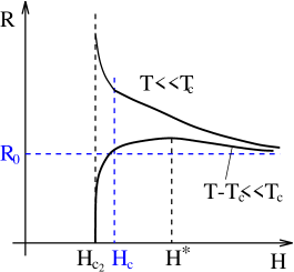
FIG. 10.: Resistivity of the granulated superconductors as a function of the magnetic field at fixed temperatures in different regimes.

Qualitatively, the results are summarized in Fig. 9, where typical curves for the low temperatures $T\ll T_{c}$ and temperatures close to $T_{c}$ are represented. Both the functions reach asymptotically the value of the classical resistivity $R_{0}$ only at extremely strong magnetic fields. The resistivity $R$ at low temperatures grows monotonously when decreasing the magnetic field. The function does not have any singularity at the magnetic field $H_{c}$ destroying the superconducting gap $\Delta$ in a single grain. The real transition into the superconducting state occurs at a lower field $H_{c_{2}}$. This field, in the region of parameters involved, is close to the field $H_{c}$. The resistivity $R\left(H\right)$ remains finite as $H\rightarrow H_{c_{2}}$ but its derivative diverges resulting in the infinite slope at $H=H_{c_{2}}$. The dependence of the resistivity $R$ on the magnetic field at temperatures near $T_{c}$ is more complicated. Already far from the field $H_{c}$ the superconducting fluctuations start contributing to transport and the resistivity goes down when decreasing the magnetic field. A negative magnetoresistance is possible in this region only at magnetic fields $H^{\ast}$, that can be much larger than the field $H_{c}$.

The theory developed gives a good description of existing experiments. Although the experimental systems are close to the metal-insulator transition and localization effects as well as Coulomb interaction can play an essential role, our theory, where all these effects were neglected, gives reasonable values of physical quantities and allows to reproduce the main features of experimental curves.

It was important for our calculations that the dimensionless conductance $J\gg 1$ of the sample was limited also from above, such that the inequality $J\ll\Delta_{0}/\delta$ was fulfilled. This means that the granulated structure of the superconductor was essential for us. However, the fact that the contribution of the superconducting fluctuations vanishes in the limit $T\rightarrow 0$ (AL and MT corrections are proportional to $T^{2}$) seems to be rather general and not restricted by this inequality. Apparently, the negative magnetoresistance above the critical magnetic field persists and can be possible even in conventional bulk superconductors. We leave the region of large conductances $J\gtrsim\Delta_{0}/\delta$ for a future study.

XII ACKNOWLEDGMENTS

The authors thank I. Aleiner, B. Altshuler, F. Hekking for helpful discussions in the course of the work. A support of the Graduiertenkolleg 384 and the Sonderforschungsbereich 237 is greatly appreciated. The work of one of the authors (A.I. L.) was supported by the NSF grant DMR-9812340. He thanks also the Alexander von Humboldt Foundation for a support of his work in Bochum.

REFERENCES

- [1] A. Gerber, A. Milner, G. Deutscher, M. Karpovsky, A. Gladkikh, Phys. Rev. Lett. 78, 4277 (1997).
- [2] T. Chui, P. Lindenfeld, W. L. McLean, K. Mui, Phys. Rev. Lett. 47, 1617 (1981).
- [3] V. F. Gantmakher, M. Golubkov, J. G. S. Lok, A. K. Geim, Sov. Phys. JETP, 82, 951 (1996); V. F. Gantmakher (cond-mat/9709017).
- [4] B. L. Altshuler, D. E. Khmelnitskii, A. I. Larkin, P . A. Lee, Phys. Rev. B 22, 5142 (1980).
- [5] K.B. Efetov, Sov. Phys. JETP 51, 1015 (1980).
- [6] I.S. Beloborodov and K.B. Efetov, Phys. Rev. Lett. 82, 3332 (1999).
- [7] L. G. Aslamazov and A. I. Larkin, Soviet Solid State, 10, 875 (1968).
- [8] K. Maki, Progr. Theoret. Phys. 39, 897 (1968); 40, 193 (1968); R. S. Thompson, Phys. Rev. B 1, 327 (1970).
- [9] E. Abrahams, M. Redi, J. Woo, Phys. Rev. B 1, 208, (1970).
- [10] A. A. Varlamov, G. Balesterino, E.Milani, and D.V. Livanov (cond-mat/9710175).
- [11] L.B. Ioffe, A.I. Larkin, A.A. Varlamov, and L. Yu, Phys. Rev. B 47 , 8936 (1993).
- [12] I. L. Aleiner and B. L. Altshuler, Phys. Rev. Lett. 79 (1997) 921; H. Y. Kee, I. L. Aleiner and B. L. Altshuler, Phys. Rev. B 58 (1998) 5757.
- [13] K. B. Efetov, Supersymmetry in Disoder and Chaos, Cambridge University Press, New York (1997).
- [14] I. O. Kulik and I. K. Yanson, The Josephson Effect in Superconducting Tunneling Structures, Halsted, Jerusalem, 1972.
- [15] A. A. Abrikosov, L. P. Gorkov and I. E. Dzyaloshinskii, Methods of Quantum Field Theory in Statistical Physics. (Prentice-Hall, Englewood Cliffs, NJ, 1963).
- [16] A. I. Larkin, Sov. Phys. JETP, 21, 153 (1965).
- [17] B. L. Altshuler, A. G. Aronov, A. I. Larkin, D. E. Khmelnitskii, Sov. Phys. JETP, 54, 411 (1981).
- [18] A. Schmid, Phys. Rev. 180, 527 (1969).
- [19] K.B. Efetov, Sov. Phys. JETP 67, 199 (1988).