Comprehensive study of Frohlich polaron

Abstract

A detailed study of the Fröhlich polaron model is performed on the basis of diagrammatic quantum Monte Carlo method [1]. The method is further developed both quantitatively (performance) and qualitatively (new estimators), and is enhanced by spectral analysis of the polaron Green function, within a novel approach. We present the best up to date results for the binding energy, and for the first time make available precise data for the effective mass, including the region of intermediate and strong couplings. We look at the structure of the polaron cloud and answer such questions as the average number of phonons in the cloud and their number/momentum distribution. The spectral analysis reveals non-trivial structure of the spectral density at intermediate and large coupling: the spectral continuum features pronounced peaks that we attribute to unstable excited states of the polaron.

PACS numbers: 71.38.+i, 02.70.Lq, 05.20.-y

I Introduction

The polaron problem (for an introduction see Ref. [2]) has originally emerged in the solid state physics as a problem of electron moving in a (dielectric) medium. It became clear, however, that this problem is of essential general-physical interest, as a model of a quantum object strongly coupled to an environment. Starting from the work of Landau [3], the polaron problem has been attracting a permanent attention, serving as a testing ground of new non-perturbative methods.

The most popular model in the polaron problem is the so-called Fröhlich Hamiltonian describing an electron coupled to non-dispersive (optical) phonons of a dielectric medium via its polarization (Plank’s constant and electron mass are set equal to unity) [4]:

$$H\,=\,H_{\mbox{e}}+H_{\mbox{ph}}+H_{\mbox{e-ph}}\;,$$ (1)

$$H_{\mbox{e}}\,=\,\sum_{\bf k}\,\frac{k^{2}}{2}\,a^{{\dagger}}_{\bf k}a_{\bf k}\;,$$ (2)

$$H_{\mbox{ph}}\,=\,\sum_{\bf q}\,\omega_{q}\,b^{{\dagger}}_{\bf q}b_{\bf q}\;,$$ (3)

$$H_{\mbox{e-ph}}\,=\,\sum_{{\bf k},{\bf q}}\,V({\bf q})\,\left(b^{{\dagger}}_{\bf q}-b_{-{\bf q}}\right)\,a^{{\dagger}}_{{\bf k}-{\bf q}}a_{\bf k}\;,$$ (4)

$$V({\bf q})\,=\,i\,\left(2\sqrt{2}\alpha\pi\right)^{1/2}\,\frac{1}{q}\;.$$ (5)

In Eqs. (1-5), $a_{\bf k}$ and $b_{\bf q}$ are the annihilation operators for the electron with momentum $\bf k$ and for the phonon with momentum $\bf q$, respectively, $\omega_{q}\equiv\omega_{0}$ is the $\bf q$-independent phonon frequency, which can be set equal to unity without loss of generality, $\alpha$ is a dimensionless coupling constant.

Despite a lot of work addressed to the Fröhlich Hamiltonian, the model is still far from being completely understood. In the most interesting region - at intermediate and large values of $\alpha$, almost all available treatments are of variational character. Hence, these treatments, even if consistent with each other, can not guarantee quantitative and qualitative reliability of the results. Moreover, some treatments are known to be in qualitative disagreement with the others. As a characteristic example, note that certain approaches suggest that the polaron states at small and large $\alpha$’s are of qualitatively different nature, and there should occur a sort of phase transition in the parameter $\alpha$ [5, 6, 7, 8, 9, 10, 11] (see, however, discussion in Ref. [12]). The study of such important issues as electron $Z$-factor and the structure of the polaronic cloud was also restricted to the perturbation theory and variational treatments at small momenta [13, 14, 15, 16]. It remained unclear what are the limits of applicability of these results, and whether they correctly describe the physics of polarons in the most important range of intermediate $\alpha$.

Recently, a method of diagrammatic quantum Monte Carlo (MC) was developed, which is very efficient for the polaron-like problems [1]. The method allows direct simulation of entities specified in terms of (positive definite) diagrammatic expansions. In Ref. [1] the polaron Green function was simulated, and the results were used to extract the polaron spectrum.

In the present paper, we employ the diagrammatic Monte Carlo scheme of Ref. [1] for a detailed study of the Fröhlich model. We significantly enhanced the original scheme by (i) introducing $N$-phonon Green functions (with $2N$ external phonon lines), which are simulated in one and the same MC process with the ordinary ($0$-phonon) Green function, (ii) developing a powerful procedure of spectral analysis of the Green function. The $N$-phonon Green functions allow us to consider the structure of the phonon cloud and facilitate obtaining polaron parameters at large $\alpha$, where the polaron is essentially a many-phonon object. In particular, direct estimators for the energy, effective mass, group velocity, and $Z$-factors can be constructed. The spectral analysis of the Green function gives the most complete information about the polaron, including the possibility to reveal stable and metastable excited states, if any.

The paper is organized as follows. In Section II we introduce the set of Green functions, describe the corresponding diagrammatic series, and discuss how they are related to the polaron parameters. In Section III we describe qualitatively the Monte Carlo procedure [the quantitative discussion of the updates is given in the Appendix A]. The calculated properties of the polaron (energy, effective mass, structure of the polaronic cloud, ets.) are presented in Section IV. In Section V we analyze excited states of the polaron by restoring the spectral density of the Green function by a novel method of the spectral analysis [detailed description of the method is presented in Appendix B].

II Green functions and diagrams

In this section we introduce basic entities and establish their relations, which will be utilized in the rest of the paper.

We start with the standard Green function of the polaron in the momentum (${\bf k}$) – imaginary-time ($\tau$) representation:

$$G({\bf k},\tau)\,=\,\langle\mbox{vac}|\,a_{\bf k}(\tau)a^{{\dagger}}_{\bf k}(0)\,|\mbox{vac}\rangle\;,\;\;\tau\geq 0\;,$$ (6)

$$a_{\bf k}(\tau)\,=\,e^{H\tau}a_{\bf k}e^{-H\tau}\;.$$ (7)

Here $|\mbox{vac}\rangle$ is the vacuum state.

The physical information that $G({\bf k},\tau)$ contains is clear from the expansion

$$G({\bf k},\tau)\,=\,\sum_{\nu}\,|\langle\nu|a^{{\dagger}}_{\bf k}|\mbox{vac}\rangle|^{2}\,e^{-\left(E_{\nu}({\bf k})-E_{0}\right)\tau}\;,$$ (8)

where $\{|\nu\rangle\}$ is a complete set of eigenstates of the Hamiltonian $H$ in the sector of given ${\bf k}$, i.e.  $H\,|\nu({\bf k})\rangle=E_{\nu}({\bf k})\,|\nu({\bf k})\rangle$,  $H\,|\mbox{vac}\rangle=E_{0}\,|\mbox{vac}\rangle$. Since in our model $E_{0}=0$, we omit it below. Rewriting Eq. (8) as

$$G({\bf k},\tau)\,=\,\int_{0}^{\infty}d\omega\,g_{\bf k}(\omega)\,e^{-\omega\tau}\;,$$ (9)

$$g_{\bf k}(\omega)\,=\,\sum_{\nu}\,\delta(\omega-E_{\nu}({\bf k}))\;|\langle\nu|a^{{\dagger}}_{\bf k}|\mbox{vac}\rangle|^{2}\;,$$ (10)

one defines the spectral function $g_{\bf k}(\omega)$ which has poles (sharp peaks) at frequencies corresponding to stable (metastable) particle-like states. Hence, if at a given ${\bf k}$ there exists a stable polaron with the energy $E({\bf k})$, the spectral function reads

$$g_{\bf k}(\omega)\,=\,Z^{({\bf k})}\,\delta(\omega-E({\bf k}))\,+\,\ldots\;,$$ (11)

where

$$Z^{({\bf k})}\,=\,|\,\langle\mbox{~{}polaron~{}}({\bf k})~{}|\mbox{~{}free electron~{}}({\bf k})~{}\rangle\,|^{2}\;.$$ (12)

Moreover, if the polaron state is the ground state, its energy and $Z$-factor are “projected out” by the Green function behavior at long times:

$$G({\bf k},\tau\gg\omega_{0}^{-1})\;\to\;Z^{({\bf k})}\,e^{-E({\bf k})\tau}\;.$$ (13)

Along with the standard polaron Green function (6), it is reasonable to introduce the $N$-phonon Green function

$$G_{N}({\bf k},\tau;\,{\bf q}_{1},\ldots,{\bf q}_{N})\,=\,\langle\mbox{vac}|\,b_{{\bf q}_{N}}({\tau})\cdots b_{{\bf q}_{1}}({\tau})\,a_{\bf p}(\tau)a^{{\dagger}}_{\bf p}(0)\,b^{{\dagger}}_{{\bf q}_{1}}(0)\cdots b^{{\dagger}}_{{\bf q}_{N}}(0)|\mbox{vac}\rangle\;,\;\;{\bf p}\,=\,{\bf k}-\sum_{j=1}^{N}{\bf q}_{j}\;.$$ (14)

Relations (8-13) are readily generalized to the case of $N$-phonon Green function. In particular, the $N$-phonon $Z$-factor for the stable (groundstate) polaron with momentum ${\bf k}$,

$$Z^{({\bf k})}_{N}({\bf q}_{1},\ldots,{\bf q}_{N})\,=\,|\,\langle\mbox{~{}polaron~{}}({\bf k})~{}|\mbox{~{}free electron~{}}({\bf p})\,+\,\mbox{free phonons~{}}({\bf q}_{1},\ldots,{\bf q}_{N})~{}\rangle\,|^{2}\;$$ (15)

[the momentum ${\bf p}$ is defined as in Eq. (14)], is given by

$$G_{N}({\bf k},\tau\gg\omega_{0}^{-1};\,{\bf q}_{1},\ldots,{\bf q}_{N})\;\to\;Z^{({\bf k})}_{N}({\bf q}_{1},\ldots,{\bf q}_{N})\;e^{-E({\bf k})\tau}\;.$$ (16)

Our MC procedure of simulating Green functions will utilize a standard diagrammatic expansion - Matsubara technique at $T=0$. The diagrams (see Figs. 1, 2) are built of the following elements:

FIG. 1.: A $0$-phonon diagram.

FIG. 2.: A $2$-phonon diagram. Note, that disconnected phonon lines always appear in pairs (labels A and B), both lines in a pair having the same momentum.

(i) free-electron propagator (solid line)

$$G^{(0)}({\bf p},\tau_{2}-\tau_{1})\,=\,\exp[-\frac{p^{2}}{2}(\tau_{2}-\tau_{1})]\;,$$ (17)

(ii) phonon propagator (dashed line)

$$D({\bf q},\tau_{2}-\tau_{1})\,=\,\exp[-\omega_{q}(\tau_{2}-\tau_{1})]\;,$$ (18)

(iii) vertex factor $V({\bf q})$ ascribed to the vertex formed by a phonon propagator (with the momentum ${\bf q}$) and two adjacent electron propagators. External lines of diagrams arise from the operators standing in Eqs. (6), (14) and their times and momenta are defined accordingly. Momenta of the internal lines are free up to the momentum conservation constraint at each vertex. To obey this constraint, we choose phonon momenta to be free, fixing thus the momenta of the electron lines. Times ascribed to the line ends are subject to the chronologization constraint: The time of the left end is $0$, the time of the right diagram end is $\tau$, times of the vertexes must increase along the global electron line, directed from $0$ to $\tau$. Integration over all free parameters of the diagrams is assumed, within the domains consistent with the constraints.

Upon the formulation of the diagrammatic rules, it is reasonable to introduce the irreducible $N$-phonon Green function, $\tilde{G}_{N}$, which consists only of irreducible diagrams. [By irreducible diagrams we understand those ones that do not contain phonon lines decoupled from the electron.] ¿From this definition it is clear that the reducible part of the $N$-phonon Green function, $G_{N}-\tilde{G}_{N}$, is a sum of products of irreducible functions $\tilde{G}_{N^{\prime}}$, $N^{\prime}<N$, and free phonon propagators. Therefore, the reducible part does not contribute to the large-$\tau$ asymptotics of $G_{N}$ [because of extra factors $e^{-\omega_{0}\tau}$ coming from the disconnected phonon propagators], and, in particular, Eq. (16) holds true for $\tilde{G}_{N}$ as well.

It is usefull then to consider the following function:

$$P({\bf k},\tau)\,=\,G({\bf k},\tau)+\sum_{N=1}^{\infty}\int d{\bf q}_{1}\cdots d{\bf q}_{N}\,\tilde{G}_{N}({\bf k},\tau;\,{\bf q}_{1},\ldots,{\bf q}_{N})$$ (19)

[Note, that if $\tilde{G}_{N}\to G_{N}$, this expression would be singular at $\tau\to 0$ because of the divergence of the integrals for disconnected phonon propagators]. The function $P$ is readily calculated by our MC procedure (see next sections) and, according to (13), (16), satisfies the relation

$$P({\bf k},\tau\gg\omega_{0}^{-1})\;\to\;e^{-E({\bf k})\tau}\;.$$ (20)

Here we took into account the completeness relation

$$Z^{({\bf k})}_{0}+\sum_{N=1}^{\infty}\int d{\bf q}_{1}\cdots d{\bf q}_{N}\,Z^{({\bf k})}_{N}({\bf q}_{1},\ldots,{\bf q}_{N})\,=\,1\;.$$ (21)

Eqs. (20), (21) imply that the lowest level $E({\bf k})$ is non-degenerate. Otherwise one should introduce degeneracy factors to the right-hand sides of the equations.

III Diagrammatic Quantum Monte Carlo

In the previous work [1, 17] it has been shown how to sum convergent (and arbitrary otherwise) diagrammatic series numerically without systematic errors. In this section we outline the basic numerical procedure of evaluating series for various Green functions described in the previous section [the details being discussed in the Appendix A], and introduce a number of estimators, that render the evaluation process significantly more efficient.

Suppose that we are interested in the function $Q(\{y\})$, which depends on a set of variables $\{y\}$, and which is given in terms of a series of integrals with an ever increasing number of integration variables:

$$Q(\{y\})\,=\,\sum_{m=0}^{\infty}\sum_{\xi_{m}}\int dx_{1}\cdots dx_{m}\,{\cal D}_{m}(\xi_{m},\{y\},x_{1},\ldots,x_{m})\;.$$ (22)

Here $\xi_{m}$ indexes different terms/diagrams of the same order $m$. The term $m=0$ is understood as a certain function of $\{y\}$. Both external $\{y\}$ and internal $\{x_{i}\}$ variables are allowed to be either continuous or discrete; in the latter case integrals are understood as sums. Diagrammatic MC process is a numeric procedure based on the Metropolis principle [18] that samples various diagrams in the parameter space $(\{y\},m,\xi_{m},\{x\}_{m})$ and collects statistics for $Q(\{y\})$ in such a way that the final result converges to the exact answer. The process has very much in common with the Monte Carlo simulation of a distribution given by a multi-dimensional integral. Nevertheless, there is an essential difference associated with the fact that integration multiplicity in the expansion Eq. (22) is varying.

Summing the series for $Q(\{y\})$ is the process of sequential stochastic generation of diagrams described by functions ${\cal D}_{m}$, Eq. (22). The MC process consists of a number of elementary updates falling into two qualitatively different classes: (I) those which do not change the type of the diagram (change the values of arguments in ${\cal D}_{m}$, but not the function itself), and (II) those which do change the diagram order. The set of elementary updates and their implementation is problem-specific; the only necessary requirements are ergodicity, i.e., given two arbitrary diagrams it takes finite number of updates to transform one to another, and detailed balance, i.e., diagrams contribute to the statistics according to ratio of their ${\cal D}$-functions. In the Appendix A we describe a set of updates which we find to work very efficiently. However, considering enormous freedom in constructing various updates, we have little doubts that they may not be further improved.

Though Green function contains complete information associated with the polaron spectrum, and the accumulation of the histogram for $G$ is straightforward, it is reasonable to introduce certain direct estimators, including one for the Green function itself. These estimators substantially enhance the accuracy of calculations and/or allow collecting more information during one MC run (by “spreading” the data to the different values of the external parameters).

A Estimators for effective mass, group velocity, and energy

We start with the family of estimators that are constructed in accordance with the following standard MC rule. Suppose we have some quantity $A$ specified by the diagrammatic expansion

$$A\,=\,\sum_{\nu}\,{\cal D}^{(A)}_{\nu}\;,$$ (23)

where ${\cal D}^{(A)}_{\nu}$’s are the diagrams for $A$ which are parametrized by internal variables denoted by the unified index $\nu$, and the summation over $\nu$ is understood as the summation over discrete variables and integration over the continuous ones. Suppose next that all ${\cal D}^{(A)}_{\nu}$’s are positive definite and we have a MC process of generation of random $\nu$ with probability density given by ${\cal D}^{(A)}_{\nu}$. Then, if some quantity $B$ is specified by a (similar) diagrammatic expansion

$$B\,=\,\sum_{\nu}\,{\cal D}^{(B)}_{\nu}\;,$$ (24)

the estimator for the ratio $B/A$ is given by

$$\frac{B}{A}\,=\,\left(\sum_{\mbox{MC}_{A}\{\nu\}}Q_{\nu}\right)\,/\,\sum_{\mbox{MC}_{A}\{\nu\}}1\;,\;\;$$ (25)

$$Q_{\nu}\,=\,\frac{{\cal D}^{(B)}_{\nu}}{{\cal D}^{(A)}_{\nu}}\;.$$ (26)

Here $\mbox{MC}_{A}\{\nu\}$ means the set of ${\nu}$’s generated during the MC run. Commonly, the quantities $A$ and $B$ in Eq. (25) are, respectively, the partition function and an observable. We, however, will use this relation in a somewhat different context. For one thing, in our case $A$ and $B$ can correspond to one and the same Green function, but at different values of external parameters (say, momentum or coupling constant). This way we are able to obtain results for a number of different values of the external parameters from a MC process for just one fixed set of parameters. We can also directly calculate derivatives with respect to the external parameters. To this end we should analytically take the corresponding limit from both sides of Eq. (25).

Let us obtain estimators for the effective mass, $m_{*}$, and group velocity, ${\bf v}({\bf k})=\partial E({\bf k})/\partial{\bf k}$. First we note that ($\tau\to\infty$,  $\lambda\to 0$)

$$\frac{P({\bf k}+\lambda{\bf\hat{e}},\tau)}{P({\bf k},\tau)}\;\to\;\left\{\begin{array}[]{ll}\exp(-\lambda^{2}\tau/2m_{*})\;,&k=0\,,\\ \exp(-\lambda{\bf\hat{e}}{\bf v}({\bf k})\tau)\;,&k\neq 0\,,\end{array}\right.$$ (27)

where ${\bf\hat{e}}$ is a unit vector. Considering the denominator and the numerator of the left-hand side of Eq. (27) as $A$ and $B$ (respectively), we can take advantage of Eqs. (25) and (26). The function $Q$ is given by

$$Q\,=\,\prod_{j}\exp\{-\frac{1}{2}[({\bf p}_{j}+\lambda{\bf\hat{e}})^{2}-{\bf p}_{j}^{2}](\Delta\tau)_{j}\}\;.$$ (28)

Here $j$ numerates free-electron propagators of a given diagram for $P({\bf k},\tau)$; ${\bf p}_{j}$ is the momentum corresponding to the propagator $j$, and $(\Delta\tau)_{j}$ is the length of this propagator. Eq. (28) immediately follows from the fact that the series for $P({\bf k}+\lambda{\bf\hat{e}},\tau)$ can be obtained from the series for $P({\bf k},\tau)$ by adding the momentum $\lambda{\bf\hat{e}}$ to all free-electron propagators. As we are interested only in the limit $\lambda\to 0$, we can expand Eq. (28) in powers of $\lambda$:

$$Q\,=\,1-\lambda\tau({\bf\hat{e}}\overline{\bf p})-\frac{\lambda^{2}}{2}\tau+\frac{\lambda^{2}}{2}\tau^{2}({\bf\hat{e}}\overline{\bf p})^{2}+{\cal O}(\lambda^{3})\;,$$ (29)

where $\overline{\bf p}$ is the mean electronic momentum of the given diagram

$$\overline{\bf p}\,=\,\frac{1}{\tau}\sum_{j}{\bf p}_{j}\,(\Delta\tau)_{j}\;.$$ (30)

Comparing Eq. (29) with the corresponding expansions of the right-hand side of Eq. (27), we arrive to the following estimators

$$\left\langle\,\overline{\bf p}\,\right\rangle_{\mbox{MC}}\;\to\;{\bf v}({\bf k})\;\;\;\;\;\;\;(\tau\to\infty)\;,$$ (31)

$$1-\frac{\tau}{3}\,\left\langle\,(\overline{\bf p})^{2}\,\right\rangle_{\mbox{MC}}\;\to\;\frac{1}{m_{*}}\;\;\;\;\;\;\;(\tau\to\infty)\;,$$ (32)

where $\langle\,\ldots\,\rangle_{\mbox{MC}}$ means MC averaging in accordance with Eq. (25).

A special care should be taken for treating the time of the Green function as an external parameter of the diagrams (in the sense adopted in this section). The problem is that relations (25-26) imply that the internal parameters of diagrams ${\cal D}_{\nu}^{(A)}$ and ${\cal D}_{\nu}^{(B)}$ have one and the same domain of definition, otherwise the ratio (26) is not correctly defined. Meanwhile, the domain of internal times of diagrams directly depends on the external time. To circumvent this problem, one can introduce scaled internal times by simple relation $\tau_{i}=\tau\tilde{\tau}_{i}$, where $\tau$ is the external time (length of diagram in time), $\tau_{i}$ is an internal time variable (position in time of an electron-phonon vertex), and $\tilde{\tau}_{i}\in[0,1]$ is the corresponding scaled time variable with the domain of definition independent of $\tau$.

Now it is easy to obtain a direct estimator for the polaron energy. To this end we start from the relation

$$\frac{P({\bf k},(1+\lambda)\tau)}{P({\bf k},\tau)}\;\to\;e^{-\lambda E({\bf k})\tau}\;\;\;\;\;\;(\tau\to\infty)$$ (33)

and proceed analogously to Eqs. (27-32). In this case for the function $Q$ we have

$$Q\,=\,(1+\lambda)^{N}\left(\prod_{j}\exp[-\lambda\frac{p_{j}^{2}}{2}(\Delta\tau)_{j}]\right)\left(\prod_{s}\exp[-\lambda\omega_{0}(\Delta\tau)_{s}]\right)\;,$$ (34)

where indexes $j$ and $s$ stand for the electron and phonon propagators, respectively, and $N$ is the number of integrations over times (or, equivalently, number of interaction vertexes) in a given diagram. Then, in the limit $\lambda\to 0$, we expand the right-hand sides of Eqs. (33-34) up to terms proportional to $\lambda$, and in accordance with Eqs. (25-26) arrive to the estimator

$$\frac{1}{\tau}\,\left\langle\,\sum_{j}\,\frac{p_{j}^{2}}{2}(\Delta\tau)_{j}\,+\,\sum_{s}\,\omega_{0}(\Delta\tau)_{s}\,-N\,\right\rangle_{\mbox{MC}}\;\to\;\;\;E({\bf k})\;\;\;\;\;\;\;\;(\tau\to\infty)\;.$$ (35)

B Reweighting

We will also employ the reweighting technique [19], which allows one to utilize the statistics being generated for some given set of external variables, $\xi$, for calculations at a different set, $\xi^{\prime}$. In terms of the diagrammatic Monte Carlo, this technique is based on the relation

$$\sum_{\mbox{MC}\{\nu\}|_{\xi^{\prime}}}Q_{\nu}(\xi^{\prime})\;=\,\sum_{\mbox{MC}\{\nu\}|_{\xi}}\frac{{\cal D}_{\nu}(\xi^{\prime})}{{\cal D}_{\nu}(\xi)}\,Q_{\nu}(\xi^{\prime})\;,$$ (36)

where $Q_{\nu}$ is any quantity summed over MC statistics. [We omitted superscript $A$ at ${\cal D}_{\nu}$ since it is not relevant here.] The relation (36) follows from the fact that the MC statistics for the set $\xi^{\prime}$ involves the same (in the sense of structure and the values of internal parameters) diagrams as the statistics for the set $\xi$. The difference is only due to a different probability to generate a diagram with the set $\xi$ rather than $\xi^{\prime}$. This difference can be taken into account analytically by the corresponding ratio, which immediately leads to (36).

In our case, typical external parameters are the interaction constant and the polaron momentum: $\xi=(\alpha,{\bf k})$. The corresponding ratio of the diagrams is

$$\frac{{\cal D}_{\nu}(\alpha^{\prime},{\bf k}^{\prime})}{{\cal D}_{\nu}(\alpha,{\bf k})}\,=\,\left(\frac{\alpha^{\prime}}{\alpha}\right)^{N/2}\prod_{j}\exp\{-[({\bf k}^{\prime}-{\bf k})^{2}+2{\bf p}_{j}({\bf k}^{\prime}-{\bf k})](\Delta\tau)_{j}/2\}\,=\,\left(\frac{\alpha^{\prime}}{\alpha}\right)^{N/2}e^{-[({\bf k}^{\prime}-{\bf k})^{2}/2+\overline{\bf p}({\bf k}^{\prime}-{\bf k})]\tau}\;.$$ (37)

This relation allows to get many points at different ${\alpha}^{\prime}$ and ${\bf k}^{\prime}$, at no extra cost in CPU time, while performing MC at a given set of ${\alpha}$ and ${\bf k}$ (cf. Ref. [19]).

C Exact estimator for Green’s function

Calculation of the Green function by means of histogram, though is simple and natural, involves an apparent shortcoming, associated with the finite width of the histogram cell. There is always a competition between the decreasing systematic error by making the size of the cell smaller, and the increasing statistical accuracy, which requires increasing the size of the histogram cell. This problem can be solved by introducing an exact (free of systematic errors) estimator for the Green function, as follows from a generic consideration presented below.

Given some function $A(\xi_{0})$ of an external variable/set of variables $\xi_{0}$, specified with the (positive definite) diagrammatic expansion

$$A(\xi_{0})\,=\,\sum_{\nu}\,{\cal D}_{\nu}(\xi_{0})\equiv\int d\xi\sum_{\nu}\,{\cal D}_{\nu}(\xi)\delta(\xi-\xi_{0})\;,$$ (38)

[considering a general case, we do not assume that the domain of definition of $\nu$ is independent of $\xi$] and having arranged a MC process of generating configurations $\{\nu,\xi\}$ with the probability density proportional to ${\cal D}_{\nu}(\xi)$, we would like to construct an estimator $a_{\xi_{0}}$ the average of which over the MC process gives (up to a global normalization factor) the function $A(\xi_{0})$. Let us look for $a_{\xi_{0}}$ in the following form

$$a_{\xi_{0}}(\nu,\xi)\,=\,\left\{\begin{array}[]{ll}q(\nu){\cal D}_{\nu}(\xi_{0})/{\cal D}_{\nu}(\xi),&\;\mbox{if}~{}\xi\in\Gamma_{0}~{}\mbox{and}~{}{\cal D}_{\nu}(\xi)\neq 0\;,\\ 0\;,&\mbox{otherwise}\;.\end{array}\right.$$ (39)

Here $\Gamma_{0}$ is some finite domain in the space of variable $\xi$ including the point $\xi_{0}$, $q(\nu)$ is some function to be defined later. [We adopt a convenient and consistent with the MC procedure convention that ${\cal D}_{\nu}(\xi)\equiv 0$, if $\xi$ is out of the range of definition of the corresponding diagram.] ¿From Eq. (39) we have

$$\left\langle\,a_{\xi_{0}}\,\right\rangle_{\mbox{MC}}\,\equiv\,C\sum_{\nu}\int d\xi\,a_{\xi_{0}}(\nu,\xi)\,{\cal D}_{\nu}(\xi)\,=\,C\sum_{\nu}\,q(\nu)\,{\cal D}_{\nu}(\xi_{0})\int_{\xi\in\Gamma_{0},~{}{\cal D}_{\nu}(\xi)\neq 0}d\xi$$ (40)

where

$$C^{-1}\,=\,\sum_{\nu}\int d\xi\,{\cal D}_{\nu}(\xi)$$ (41)

is the normalization factor for the distribution of the random pairs $(\nu,\xi)$ induced by the series (38). ¿From Eq. (40) it is seen that if we choose

$$q^{-1}(\nu)\,=\,\int_{\xi\in\Gamma_{0},~{}{\cal D}_{\nu}(\xi)\neq 0}d\xi\;$$ (42)

[note that, according to (39), the definition of $q(\nu)$ is relevant only when ${\cal D}_{\nu}(\xi_{0})\neq 0$, and that $q^{-1}(\nu)\neq 0$, since at least small neighborhood of the point $\xi_{0}$ contributes to the integral], then

$$\left\langle\,a_{\xi_{0}}\,\right\rangle_{\mbox{MC}}\,=\,CA(\xi_{0})\;.$$ (43)

The particular form of the estimator for the Green function is readily obtained by identifying $\xi$ with $\tau$, and noting that the ratio of diagrams standing in Eq. (39) is given in this case by Eq. (34). As the domain of definition of any diagram with respect to $\tau$ is independent of the diagram structure: $\tau\in[0,\infty]$, the factor $q$ in Eq. (39) is simply proportional to the inverse size of the interval $\Gamma_{0}$. The choice of $\Gamma_{0}$ for each particular $\tau_{0}$ is arbitrary, being a matter of taste and convenience.

D Improved estimators for phonon statistics

Collecting statistics for the phonon cloud can be significantly improved by a trick described below.

We start with noting that in the case of $\tau\to\infty$, which is relevant to the ground-state properties, the set of all $N$-phonon diagrams possesses a certain symmetry. To reveal this symmetry, we transform diagrams to the circular representation by the rules illustrated in Fig. 3.

FIG. 3.: Correspondence between the standard and circular representations of diagrams.

The transformation involves “gluing” the outer ends of the electron line, as well as the outer ends of pairs of (corresponding to each other) external phonon lines. It is easy to check that the procedure is consistent with the definitions of propagators, Eqs. (17, 18). In the limit of large $\tau$, which we are interested in, the probability to find a phonon propagator with length $>\tau/2$ is vanishingly small. That is why we may omit orientation, understanding the time length of phonon propagator as the length of the smallest arc between its ends. With the same accuracy, in the limit $\tau\to\infty$, we may ignore the pairs of phonon lines like the one shown in Fig. 3(c), which do not have unambiguous circular counterparts.

It is worth noting that circular diagrams naturally occur in a finite-temperature technique (cf., e.g., Ref. [20]), where the circumference $\tau$ has a meaning of inverse temperature.

Within the circular representation the symmetry necessary for constructing improved estimators is clearly seen. Indeed, a circular diagram represents a whole class of plain diagrams, due to its independence of the position of the point corresponding to the ends of the plain diagram.

Thus, having generated a certain plain diagram and associating it with the corresponding circular diagram, one effectively produces a whole class of diagrams to be included into the statistics.

In practice, the procedure is as follows. Let index $i=1,\dots,N_{e}$ label electron propagators in the circular diagram; we thus split the diagram into $N_{e}$ pieces each having duration $\Delta\tau_{i}$ in time, $\sum_{i=1}^{N_{e}}\Delta_{i}=\tau$. When the circular diagram is cut anywhere on the interval $\Delta\tau_{i}$ we obtain a contribution to $\tilde{G}_{N_{i}}({\bf k},\tau;{\bf q}_{1}^{(i)},\dots,{\bf q}_{N_{i}}^{(i)})$, where $N_{i}$ is the number of phonon propagators which are cut along with the electron propagator on this interval, and $\{{\bf q}_{i}\}$ are their momenta. An estimator for the integrated N-phonon Z-factor is found then to be

$$Z^{({\bf k})}_{N}\equiv\int\dots\int\prod_{j=1}^{N}d{\bf q}_{j}Z^{({\bf k})}_{N}({\bf q}_{1},\dots,{\bf q}_{N})=\left\langle\sum_{i=1}^{N_{e}}{\Delta\tau_{i}\over\tau}\delta_{N_{i},N}\right\rangle_{MC}\;,$$ (44)

i.e., due to time invariance of the circular representation each interval contributes to the statistics according to its duration in time. The one-phonon distribution function within the N-phonon states manifold is given by

$$F^{({\bf k})}_{N}({\bf q})\equiv\int\dots\int\prod_{j=2}^{N}d{\bf q}_{j}Z^{({\bf k})}_{N}({\bf q},{\bf q}_{2},\dots,{\bf q}_{N}) \equiv {1\over N}\sum_{l=1}^{N}\int\dots\int\prod_{j\neq l}^{N}d{\bf q}_{j}Z^{({\bf k})}_{N}({\bf q}_{1},\dots,{\bf q}_{l}={\bf q},\dots,{\bf q}_{N})$$ (45)

$$= \left\langle\sum_{i=1}^{N_{e}}{\Delta\tau_{i}\over\tau}\>\delta_{N_{i},N}\>{1\over N_{i}}\sum_{j=1}^{N_{i}}\delta({\bf q}_{j}-{\bf q})\right\rangle_{MC}\;,$$ (46)

Obviously, $Z^{({\bf k})}_{N}=\int d{\bf q}F^{({\bf k})}_{N}({\bf q})$. Summing over all $N$ we obtain the one-phonon distribution function

$$F^{({\bf k})}({\bf q})=\sum_{N=1}^{\infty}F^{({\bf k})}_{N}({\bf q})\;.$$ (47)

IV Numeric results

A Groundstate energy and effective mass

In Fig. 4 we present our results for the bottom of the band

FIG. 4.: Bottom of the polaron band $E_{0}$ as a function of $\alpha$. The error bars are much smaller than the point size.

$E_{0}$ as a function of $\alpha$ in a wide region of coupling strengths. The data are compared with Feynman’s variational treatment [13] to demonstrate the remarkable accuracy of the Feynman’s approach to the polaron energy. We thus conclude that just a simple extrapolation between the second-order perturbative result $E_{0}=-\alpha-1.26(\alpha/10)^{2}$ and Feynman’s strong-coupling variational estimate $E_{0}=-\alpha^{2}/3\pi-2.83$ [such an extrapolation is very close to Feynman’s variational treatment in the whole range of $\alpha$’s] yields quite satisfactory approximation for $E_{0}(\alpha)$.

In Fig. 5 accurate data for the effective mass are presented up

FIG. 5.: Effective mass as a function of coupling parameter. Our MC data (circles interpolated by solid line) are compared with perturbation theory and strong-coupling-limit results (dashed lines), Feynman’s approach (squares), and Feranchuk et. al. variational approach (dimonds).

to $m_{*}\sim 1000$ [For larger $m_{*}$’s the Fröhlich model is not realistic anyway since the phonon dispersion becomes relevant]. At $\alpha\leq 9$ the statistics were collected at integer values of $\alpha$ with reweighting (in accordance with the procedure described in the previous section) to corresponding finite intervals (see the plot). At $\alpha>9$ the reweighting procedure proved to be ineffective.

Let us compare the data for $m_{*}$ with the small- and strong-coupling analytic results. At small $\alpha$’s, the formula $m_{*}=(1-\alpha/6)^{-1}$, known to coincide with the perturbation expansion up to the second order [4, 16, 14], works well up to $\alpha\approx 2$. In contrast to the case of $E_{0}$, the strong-coupling limit [21] $m_{*}=\alpha^{4}/48$ drastically overestimates the effective mass in the whole range of physically interesting $\alpha$’s. Feynman’s variational technique works better, but still with a considerable deviation (up to $50$% ) in the region $5<\alpha<10$.

Almost the same degree of accuracy gives variational treatment by Feranchuk, Fisher, and Komarov [11]. An important point about this treatment, however, is that it suggests a phase transition from “light” to “heavy” polaron at $\alpha$ close to $7.5$, which should lead to an especially rapid increase of $m_{*}$ just after $\alpha=7.5$. In this connection, we note that our curve $m_{*}(\alpha)$ is essentially smooth and does not suggest any sort of phase transition or sharp cross-over. [The results of more deep numeric study of the possibility of the phase transition are presented in the next (sub)sections.]

B Structure of polaronic cloud

In this subsection we present our results for the electron Z-factor, or $Z^{({\bf k})}_{0}$, for ${\bf k}=0$ as a function of the coupling strength in the region of small and intermediate $\alpha$ (for $\alpha>10$, the bare electron weight in the polaron ground state becomes vanishingly small), and for $\alpha=1$ as a function of momentum up to the end-point. We study also, how the distribution of phonons in the ground state, $Z_{N}^{(0)}$, and the average number of phonons, $\bar{N}=\sum_{N=1}^{\infty}NZ_{N}^{(0)}$, evolve with $\alpha$. Finally, we show how the physics of the end-point is seen in the transformation of the one-particle distribution function $F_{\bf k}({\bf q})$, Eq. (47), and how it allows to identify the relevant self-energy diagram.

For small $\alpha$ and ${\bf k}=0$ the leading behavior is readily obtained from the perturbation theory

$$F^{(0)}_{1}({\bf q}) = {\sqrt{2}\alpha\over 4\pi^{2}}\>{\sin\theta\over[q^{2}/2+1]^{2}}dq\>d\theta\>d\varphi$$ (48)

$$Z^{(0)}_{0} = \alpha/2$$ (49)

$$Z^{(0)}_{0} = 1-\alpha/2\;,$$ (50)

We have verified that for $\alpha<1$ the perturbative results (50) are describing the data rather accurately [see also Figs. 6, 8, and dashed curves (connecting filled circles) in Fig. 11].

FIG. 6.: The bare-electron $Z^{(0)}_{0}$-factor for the ground state as a function of the coupling strength; filled circles are the MC data (with error bars smaller than point size), and the solid line is the perturbation theory result (50).

The data in Fig. 6 make it clear that perturbation theory may not be trusted for $\alpha>1$ when the bare-electron state in the polaron wave function is no longer the dominant contribution, e.g., $Z_{0}^{(0)}(\alpha=3)<0.2$. The bare electron Z-factor vanishes rather rapidly for $\alpha>3$ (the dependence $Z_{0}^{0}(\alpha)$ is faster than exponential) and becomes $<10^{-5}$ for $\alpha\geq 10$. We do not attempt to fit the data to the particular functional dependence since we believe that in the interval $3<\alpha<10$ the polaron state undergoes a smooth transformation between weak and strong coupling limits.

FIG. 7.: Partial contributions of $N$-phonon states to the polaron ground state for various values of $\alpha$. Error bars are shown, but are typically smaller than the point size. (The dashed lines are to guide an eye.)

In Fig. 7 we show the distribution of multi-phonon states in the polaron cloud at $k=0$. We see how it gradually evolves from the perturbation theory case into the strong-coupling regime. For $\alpha>10$ the data may be fit to the Gaussian distribution, but at smaller values of $\alpha$ the distribution is essentially asymmetric - it decays faster for $N>\bar{N}$ than for $N<\bar{N}$. We note, that even for $alpha=17$ the phonon number distribution is rather large which means that the polaronic cloud is essentially a superposition of states with different $N$. The effects resulting from this fact are outside the scope of the variational $\Psi^{4}$-theory and may, for example, account for the considerable deviation of the effective mass discussed above.

It is well known that polaron models often support the self-trapping phenomenon, when the ground state changes in a relatively narrow interval of parameters from light- to heavy-mass state with a sharp increase in the number of phonons contributing to the polaronic cloud. The same phenomenon was advocated for the Fröhlich model by a number of authors [5, 6, 7, 8, 9, 10, 11], including the statement that more than one stable polaron state exists in the region of intermediate $\alpha$. Clearly, if there were a sharp transformation of the polaronic ground state, it would have been immediately seen in the phonon statistics. Such a transformation might be not visible on the energy plot if the hybridization matrix element between the two competing states is not small, and their energy derivatives, $dE/d\alpha$, are close to each other at the point of crossing. However, if we are to speak about different polaronic states, then (almost by definition) their structure has to undergo an abrupt change with $\alpha$. Our data on the bare electron Z-factor $Z_{0}^{0}$ and phonon distribution functions $Z_{N}^{0}$ are evolving smoothly with $\alpha$ and thus prove continuous formation of the self-trapped state.

FIG. 8.: The average number of phonons in the polaron ground state as a function of $\alpha$. Filled circles are the MC data (error bars are smaller than the point size), the dashed line is the perturbation theory result (50), and the solid line is the parabolic fit for the strong coupling limit.

To further support this conclusion, we plot in Fig. 8 the dependence $\bar{N}$ vs $\alpha$. The crossover between the perturbative result $\bar{N}\sim\alpha/2$ of Ref. [16] and the strong-coupling limit, where $\bar{N}\sim 0.22\alpha^{2}$, demonstrates no sign of the level crossing picture. As a side remark we note that the result of Ref. [16] which predicted that perturbation theory for $\bar{N}$ works well in the intermediate range $1<\alpha\leq 6$ is not true. In fact, this law breaks down along with the perturbation theory.

FIG. 9.: The bare-electron $Z$-factor as a function of the polaron momentum up to the end point.

Consider now the evolution of the polaronic cloud with momentum as we approach the end point. [The dispersion curve $E(k)$ featuring the end point at momentum $k_{c}$ of the form $E(k\to k_{c})=E_{0}+\omega_{0}-(k-k_{c})^{2}/2m_{c}$ was calculated in Ref. [1].] Although the polaronic state is stable for $E(k)-E(0)<\omega_{0}$ the bare electron weight vanishes as $k\to k_{c}$, see Fig. 9. From this plot we estimate $k_{c}(\alpha=1)\approx 1.83$. This figure also makes it clear to what degree the earlier result that $Z_{0}^{({\bf k})}$ is momentum-independent [22] works.

With the numerical tools at hand it is possible to “visualize” the physics of the end point. In accordance with the generic Pitaevskii theory of the end point [23], in the vicinity of the end point the polaron can be considered as a (weakly) bound state of phonon, carrying almost all the momentum of the state, and a polaron with almost zero momentum. This physics is transparent from the comparison between the statistics of $N$-phonon states in the ground state and at $k\to k_{c}$ shown in Fig. 10. Evidently, the two curves can be matched by shifting the ground-state distribution by one, i.e. $Z_{N}^{(k_{c})}\approx Z_{N+1}^{0}$ (the maximum of the $Z_{N}^{(k=1.79)}$ curve is a little depleted because of the remaining finite weight $Z_{0}^{0}$ since $k<k_{c}$). It means that the polaronic state near the end point is a superposition of bound states of the phonon with momentum around $k_{c}$ and a polaron at the band bottom.

Since Fig. 10 does not tell us explicitly what are the parameters of the extra phonon present in the polaronic cloud at $k\to k_{c}$, we plot in Figs. 11 12 normalized distribution functions of phonon momenta (in $|q|$ and in the angle between $\hat{{\bf q}{\bf k}}$). It is obvious from these figures that the extra phonon momentum is concentrated around ${\bf k}$.

FIG. 10.: Partial weights $Z_{N}$ of the $N$-phonon states in the structure of the polaronic state for $\alpha=1$ at the band bottom and near the end point. (The dashed lines are to guide an eye.)

FIG. 11.: Phonon distribution functions in $q$-modulus for the ground state (filled circles) and close to the end-point for $k=1.79$ (open circles). The momentum $k_{c}$ is indicated by a bar at the q-axis. (The lines are just linear interpolations between accurate numeric points.)

FIG. 12.: Phonon distribution functions in the angle between the vectors ${\bf q}$ and ${\bf k}$ close to the end-point for $k=1.79$.

V Spectral analysis

The spectral function $g_{\bf k}(\omega)$ (10) provides important information about the system since it has poles (sharp peaks) at frequencies corresponding to stable (metastable) particle-like states. Besides, since the probability of absorption of a free electron with the momentum ${\bf k}$ into a polaron state is proportional to the spectral function, the latter can be measured experimentally by angle-resolved inverse photoemission spectroscopy.

In spite of many elaborated treatments of the properties of the polaron, the knowledge about high-energy part of the polaron spectrum is mostly limited by attempts to calculate the spectral density either by perturbation theory approaches or at strong coupling limit [24]. As both the Green function asymptotic behavior and the machinery of estimators provides information about ground state properties only, the spectral density is indispensable for the study of excited states of the system.

The spectral analysis, i.e. solving the equation (9), was performed by a novel method [detailed description of the method and testing examples are presented in Appendix II]. The most important features of the method are that it avoids distortion of equation by nonlinear terms and does not suffer from systematic errors caused by preassigned discretisation of the $\omega$-space.

To perform a joint check of the diagrammatic Monte Carlo approach and the method of spectral analysis, we compared the spectral densities obtained by our numeric calculations and by perturbation theory for zero temperature. The analytic expression for the high-energy part ($\omega>0$) of the spectral density could be obtained for the arbitrary interaction potential $V(\mid{\bf q}\mid)$ which depends on the modulus $\mid{\bf q}\mid$ of the phonon momentum. For zero polaron momentum, ${\bf k}=0$, the the imaginary part of the linear in $\alpha$ self-energy part $\Sigma(0,\omega>0)$ is

$$\mbox{Im}\Sigma(0,\omega)=-\frac{1}{\sqrt{2}\pi}\sqrt{\omega-1}\mid V(\sqrt{2(\omega-1)})\mid^{2}\theta(\omega-1).$$ (51)

(Here $\theta$ is the theta-function.) Then, using the relation $g_{\bf 0}(\omega)=-\mbox{Im}G_{{\bf k}=0}(\omega)/\pi$ and keeping only linear with respect to $\alpha$ terms one gets

$$g_{\bf 0}(\omega>0)=\frac{1}{\sqrt{2}\pi^{2}}\frac{\sqrt{\omega-1}}{\omega^{2}}\mid V(\sqrt{2(\omega-1)})\mid^{2}\theta(\omega-1).$$ (52)

The expression for the low-energy part ($\omega<0$) of the spectral density depends on the specific form of the interaction potential and we consider the perturbation theory result for the short-range interaction

$$V({\mid\bf q}\mid)\,=\,i\,\left(2\sqrt{2}\alpha\pi\right)^{1/2}\,\frac{1}{\sqrt{q^{2}+\kappa^{2}}}\;,$$ (53)

which reduces to the Frohlich one when $\kappa\to 0$. The low-energy part is the delta-functional peak

$$g_{\bf 0}(\omega<0)=\frac{\alpha}{(\kappa+\sqrt{2})^{2}}\delta\left(\omega+\alpha\frac{\sqrt{2}}{\kappa+\sqrt{2}}\right).$$ (54)

The comparison of our numeric results for the low-energy part of the Frohlich polaron ($\kappa=0$)spectral density for $\alpha=0.05$ and Eq. (54) demonstrates a perfect agreement (with the accuracy $10^{-4}$ for the polaron energy and Z-factor), whereas our results for the high-energy part (upper panel in Fig. 13) significantly deviate from the analytic curve. This is not surprising since for Frohlich polaron the perturbation theory expression is diverging as $\omega\to\omega_{0}$ and, therefore the perturbation theory breaks down. To test the case when perturbation theory is obviously valid we set $\kappa=1$ and obtained a perfect agreement for both the low- and high-energy parts of $g(\omega)$ (lower panel in Fig. 13). We note that the high-energy part of $g(\omega)$ is successfully restored by our method despite the fact that the total weight of the feature is less than $10^{-2}$ for $\alpha=0.05$.

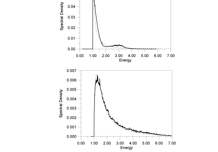
FIG. 13.: The comparison of the numeric results (solid lines) and the perturbation theory curves (dashed lines) for the spectral density of Frohlich model with $\alpha=0.05$ (upper panel) and the short-range interaction model with $\alpha=0.05$ and $\kappa=1$ (lower panel).

One can note that the main deviation of the actual spectrum of Frohlich polaron from the perturbation theory result is the extra broad peak in the actual spectral density at $\omega\sim 3.5$. To study this feature we calculated $g(\omega)$ for $\alpha=0.5$, $\alpha=1$, and $\alpha=2$ (see Fig. 14). Note, that the peak is seen for higher values of the interaction constant and its weight grows with $\alpha$. Near the threshold, $\omega=1$, the spectral density demonstrates the square-root dependence $\sim\sqrt{\omega-1}$ (see the insert).

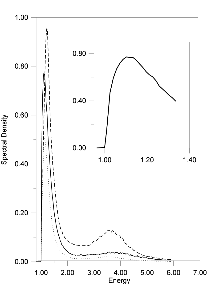
FIG. 14.: The spectral density of Frohlich polaron for $\alpha=0.5$ (dotted line), $\alpha=1$ (solid line) and $\alpha=2$ (dashed line), with energy counted from the position of the polaron. The initial fragment of the spectral density for $\alpha=1$ is shown in the insert.

To trace the evolution of the peak at higher values of $\alpha$ we calculated the spectral density for $\alpha=4$, $\alpha=6$, and $\alpha=8$ (see Fig. 15). At $\alpha=4$ the peak at $\omega\sim 3.5$ already dominates in the spectral density. Moreover, a distinct high-energy shoulder appears at $\alpha=4$, which transforms into a broad peak at $\omega\sim 9$ in the spectral density for $\alpha=6$. The spectral density for $\alpha=8$ demonstrates further redistribution of the spectral weight between different maxima without significant shift of the peak positions. One can also see that there is a high-energy shoulder which is, probably, the precursor of another peak which would appear for higher values of the interaction constant.

FIG. 15.: Evolution of spectral density with $\alpha$ in the cross-over region from intermediate to strong couplings. (The polaron ground state peak is shown only for $\alpha=8$. Note, that the spectral analysis still resolves it, despite its very small weight $<10^{-3}$.) The energy is counted from the position of the polaron.

The excited states of the polaron were studied within the frameworks of different approaches [25, 26, 27, 28, 29] by calculating optic absorption spectra. The light absorption is associated with the transitions from the polaron ground state $\phi_{0}$ with ${\bf k}=0$ and $E=E_{0}$ to the excited states $f$ with $E_{f}$ which are characterized by the presence of a finite number of real phonons along with the polaron. The optic absorption spectrum at the frequency $\omega$ is proportional to the transition probability

$$P(\omega)=2\pi\sum\langle\phi_{0}\mid\hat{O}\mid f\rangle\langle f\mid\hat{O}\mid\phi_{0}\rangle\delta(E_{0}-E_{f}+\omega).$$ (55)

(Here $\hat{O}={\bf Er}$ is the electric dipole interaction, ${\bf E}$ is the electric field.)

It was shown in the weak-coupling limit [25, 26] that the optic absorption spectrum has a broad peak with the onset separated from the polaron state by the optic phonon energy. Our calculations confirm (see Fig. 14) that there are no metastable excited states of the polaron in the weak-coupling regime.

On the other hand, in the strong-coupling limit the existence of the metastable relaxed excited state (RES), i.e. the state where the lattice readapts to the new electronic configuration and the polaron-lattice system is in the local minimum of the total energy, was predicted [27, 28, 29]. This state manifests itself as a sharp peak in the absorption spectrum which is located at the frequency equal to the energy difference $E_{\rm RES}-E_{0}$. To check the existence of RES one can study the spectral density (10) since although the matrix elements of transition probability (55) and spectral density (10) are different, both functions have to demonstrate sharp peaks at the energies of the metastable excited states. From Fig. 15 we conclude that there is no metastable excited state because the width of the peaks is comparable with the excitation energy, i.e. with the distance from the polaron ground state. Moreover, according to the strong-coupling approaches [27], the excitation energy of the RES state is proportional to $\alpha^{2}$, whereas peak positions in $g(\omega)$ with respect to $E_{0}$ do not change with $\alpha$.

The variational treatment developed in Ref. [11] suggests that in a certain region of $\alpha$ there may exist two different stable states of the polaron [the corresponding equations for variational parameters have two solutions]. Our numeric study can shed light on this situation.

To start with, let us discuss what one could observe would the two states really exist. If at some point $\alpha=\alpha_{*}$ there occurs a level crossing so that the ground state switches from one state to another, and the two states differ essentially in the number of phonons and/or in the effective mass, one would expect at the point $\alpha_{*}$ a sharp change of these quantities. The change should be almost jump-like in the case of small hybridization between the two states, and look like a smooth cross-over otherwise. Even in the case of sufficiently strong hybridization, one may distinguish between two qualitatively different cases: (i) the case when the level separation is less than $\omega_{0}$ [and thus both states are stable against decay], and (ii) the case when the upper level is in the continuum, and therefore is unstable.

Strictly speaking, in the case (ii) one can invoke the second level only in some quantitative sense, since there is no qualitative difference between the case (ii) and a situation with only one polaron state. These quantitative features could be associated with the non-monotonic behavior of the derivatives (with respect to $\alpha$) of the effective mass and/or the mean number of phonons, and, of course, another peak in the spectral density.

Our study of the spectral densities shows that the case (i) is not realized because we found that $g(0<\omega<1)=0$. Therefore, there is no excited stable state in the energy gap between the ground state energy and incoherent continuum. Instead, there are several many-phonon unstable states at energies $E_{f}-E_{0}\sim 1$, $\sim 3.5$, and $\sim 8.5$. One can speculate that these states reveal themselves in variational approaches and can be mistreated as quasi-stable states of the polaron. It should be emphasized, however, that the situation does not resemble that of the level-crossing at all, since we do not observe non-monotonic behavior of the derivatives (with respect to $\alpha$) of the effective mass and/or the mean number of phonons.

VI Acknowledgments

We are indebted to N. Nagaosa for inspiring discussions and valuable remarks. This work was supported by the Russian Foundation for Basic Research (Project 99-02-17288) and by Priority Areas Grants and Grant-in-Aid for COE research from the Ministry of Education, Science, Culture and Sports of Japan.

A Updating procedures

1 Updates of class I

Updating procedures of this class are the simplest. They mimic standard rules of simulating a given distribution function ${\cal D}_{m}$. In the present case we are dealing with quite a number of variables having different physical meaning: external variables $\{y\}$ include $\tau$, $N$, $\alpha$, and $k$, and internal variables describe the topology of the diagram (index $\xi_{m}$), times of electron-phonon vertices and momenta of phonon propagators. From this list of variables follows a set of updates simulating multi-dimensional distribution ${\cal D}_{m}$.

a Vertex shift in time

We choose at random any interaction vertex inside the graph (we exclude the diagram closing points which are updated separately), and change its time position from $\tau_{v}$ to $\tau_{v}^{\prime}$ on the interval $(\tau_{1},\tau_{2})$ between the nearest left- and right-neighbor vertices, i.e., $\tau_{1}<\tau_{v},\;\tau_{v}^{\prime}<\tau_{2}$. Let the incoming and outgoing electron momenta for the selected vertex are ${\bf p}$ and ${\bf p}+{\bf q}$. The normalized probability density to find the vertex at time $\tau_{v}^{\prime}$ is a simple exponential function

$$W(\tau_{v}^{\prime})={\Delta E\,e^{-(\tau_{v}^{\prime}-\tau_{1})\Delta E}\over 1-e^{-(\tau_{2}-\tau_{1})\Delta E}}\;,$$ (A1)

where $\Delta E=E({\bf p})-E({\bf p}+{\bf q})\mp\omega_{p}$ depending on whether the updated vertex is the left or right end of the corresponding phonon propagator, which allows a trivial solution of the equation

$$\int_{\tau_{1}}^{\tau_{v}^{\prime}}W(s)ds=r\;,$$ (A2)

in the form

$$\tau_{v}^{\prime}=\tau_{1}-{\ln\left(1-r[1-e^{-(\tau_{2}-\tau_{1})\Delta E}]\right)\over\Delta E}\;.$$ (A3)

Here and below $r$ is the random number homogeneously distributed on the unit interval. Since the new variable is selected according to the exact probability density the acceptance ratio for this update is unity.

b Change of transferred momentum angle

We choose at random any phonon propagator except those attached to the diagram ends (propagators attached to the diagram ends appear in pairs with equal momenta, thus single propagator updates do not apply to them) and change its momentum ${\bf q}\to{\bf q}^{\prime}$ so that $|{\bf q}|=|{\bf q}^{\prime}|$. Let the propagator connects vertices at times $\tau_{1}$ and $\tau_{2}$. Evaluating the average electron momentum between these vertices

$$<{\bf p}>_{\tau_{1},\tau_{2}}={\int_{\tau_{1}}^{\tau_{2}}{\bf p}(\tau)d\tau\over\tau_{2}-\tau_{1}}\;,$$ (A4)

and introducing vector ${\bf p}_{0}=<{\bf p}>_{\tau_{1},\tau_{2}}+{\bf q}$, we may write the probability density to find azimuthal and polar angles $\varphi,\theta$ between vectors ${\bf q}$ and ${\bf p}_{0}$ as

$$W(\varphi,\theta)\sim\sin(\theta)\exp\left\{-{\tau_{2}-\tau_{1}\over m}\,p_{0}q\cos\theta\right\}\;,$$ (A5)

This result is a trivial consequence of the quadratic dispersion law for the bare electron spectrum. Clearly, the new azimuthal angle is selected at random ($\varphi=2\pi r$), and $\cos\theta$ is selected according to the simple exponential function in complete analogy with Eqs. (A1) and (A3) up to trivial change of notations. The acceptance ratio is thus unity.

c Change of transferred momentum modulus

In this procedure propagators are selected as explained in the previous subsection, but now we change the modulus of the transferred momentum while keeping the polar and azimuthal angles between the vectors ${\bf p}_{0}$ and ${\bf q}$ fixed. The probability density now reads

$$W(q)\sim V(q)q^{2}\exp\left\{-{\tau_{2}-\tau_{1}\over 2m}\,[q-p_{0}\cos\theta]^{2}\right\}\sim\exp\left\{-{\tau_{2}-\tau_{1}\over 2m}\,[q-p_{0}\cos\theta]^{2}\right\}\;,$$ (A6)

where we have used explicitly the property of the Fr$\ddot{\rm o}$hlich model that $V(q)q^{2}$ is $q$-independent. By tabulating the inverse error-function we ensure fast numerical solution of the equation ${\rm errf}(z)=r$, or $z={\rm errf}^{-1}(r)$, and thus generation of the new value $q=z\sqrt{2m/(\tau_{2}-\tau_{1})}+p_{0}\cos\theta$ with acceptance ratio unity.

d Change of diagram structure

We select at random any nearest-neighbor pair of vertices inside the graph (again, the diagram closing vertices are excluded) and exchange the assignment of the phonon propagators between these vertices. Namely, if the original momentum transfer was ${\bf q}_{1}$ in vertex 1 and ${\bf q}_{2}$ in vertex 2, we suggest to change these momenta to ${\bf q}_{2}$ and ${\bf q}_{1}$ correspondingly. The acceptance ratio for this procedure depends on whether we are dealing with the left ($c=1$) or right ($c=-1$) ends of the phonon propagators

$$R=e^{-\tau[E({\bf p}+c_{1}{\bf q_{1}}-c_{2}{\bf q_{2}})-E({\bf p})-\omega_{0}(c_{1}-c_{2})]}\;,$$ (A7)

where $\tau$ is the time difference, and ${\bf p}$ is the electron momentum between the selected vertices. Clearly, this procedure effectively changes the topology of bosonic lines while keeping fixed their momenta.

e Change of diagram length in time

This procedure is done in two variants (almost identical to the procedure of shifting the vertex position in time). Consider the case when no artificial potential except the chemical potential is used. In the first variant we select the new time difference $\tau$ between the positions of the right diagram end at its left nearest neighbor vertex according to the probability density

$$W(\tau^{\prime})=\Delta E\,e^{-\tau^{\prime}\Delta E}\;,$$ (A8)

where $\Delta E=E({\bf p})+N_{z}\omega_{0}-\mu$, and ${\bf p}$ is the momentum of the last electron propagator, $\mu$ is the chemical potential, and $N_{z}$ is the number of phonon propagators attached to the diagram right end (obviously, $N_{z}$ is the same for the diagram left end). In the second variant we select new time differences between the positions of all nearest-neighbor pairs of vertices. For each such a pair the probability density is still given by Eq. (A8), where in the most general case $N_{z}$ must be understood as the number of phonon propagators which are cut when the diagram is cut anywhere between the selected pair of vertices. Notice, that the second variant requires much longer computation time; thus if the typical diagram order is very large it must be applied less frequently. In both variants the acceptance ratio is unity.

There is a bottle-neck in the time decay of the electron $P$-function, which does not allow efficient sampling of both long-time and short-time behavior and causes normalization problems at large $\alpha$, namely, $P(\tau)$ drops to almost zero vaalue at short times, and then climbs back to $P\sim 1$ before it settles to the asymptotic decay (20).

There is however a general prescription of how to eliminate such difficulties by using the so-called “guiding function” [30] or fictitious potential renormalization. This method was successfully applied recently [31] to the problem of tunneling transition amplitudes, where one is bound to collect reliable statistics which varies by orders and orders of magnitude between different points in time. The idea is to modify the statistics of suggested diagrams by introducing the acceptance ratio

$$R=A_{\mbox{fic}}(\tau_{\mbox{new}})/A_{\mbox{fic}}(\tau_{\mbox{old}})\;,$$ (A9)

and accordingly multiplying all MC estimators in the time domain by $1/A_{\mbox{fic}}(\tau)$, where the fictitious potential $A_{\mbox{fic}}(\tau)$ is arbitrary. Note, that in Eq. (A9) we are dealing with the external variable $\tau$ - the diagram length in time. In the present case the best choice would be $A_{\mbox{fic}}\sim 1/P(\tau)$. We achieve this goal by self-consistently adjusting $A_{\mbox{fic}}$ to $1/P_{MC}(\tau)$ after a certain large number of updates during the thermalization stage (here $P_{MC}(\tau)$ is the statistical result for $P(\tau)$). After thermalization stage we start collecting new statistics for $P(\tau)$ and keep $A_{\mbox{fic}}$ fixed.

f Change of coupling constant

Since the diagram weight depends on the coupling constant as $\alpha^{N_{p}}$ where $N_{p}$ is the number of phonon propagators in the diagram, all we need to do is to select new value of $\alpha$ with this power-law probability density. Normalized probability density is obtained by restricting allowed values of $\alpha$ to a certain parameter range. Acceptance ratio is unity.

g Change of external momentum

Given the average electron momentum of the diagram $\bar{\bf p}=<{\bf p}>_{0,\tau}$, see Eq. (A4), with external momentum ${\bf k}$, we define vector ${\bf p}_{0}={\bf k}-<{\bf p}>_{0,\tau}$ and write the probability density to select new external momentum ${\bf k}^{\prime}$ as

$$W({\bf k}^{\prime})\sim\exp\left\{-{\tau\over 2m}({\bf k}^{\prime}-{\bf p}_{0})^{2}\right\}\;.$$ (A10)

As before the new variable is seeded according to this probability density utilizing the tabulated error-function [see subsection A 1 c and Eq. (A6)] and thus is always accepted.

One note is in order here. Although one is allowed to change the coupling constant and the external momentum in a single MC process, it seems more efficient to keep these variables fixed instead of spreading the statistics over some range in the $({\bf k},\alpha)$ parameter space. However, the knowledge of the relative weights according to which a given diagram contributes to the statistics of various $\alpha$ and ${\bf k}$ may be utilized in collecting statistics for the finite neighborhood of the point $({\bf k}_{0},\alpha_{0})$ used in a given MC simulation. Obviously, reliable results for points other than $({\bf k}_{0},\alpha_{0})$ are obtained only provided that for typical diagrams the relative weights are of order unity. As explained in the text, this knowledge is also used in deriving estimators for the effective mass and group velocity of the polaron.

2 Updates of class II

These updates are in the heart of the method since they change the diagram order. The generic rules for constructing them are as follows [17]. Let the update $\cal A$ transform a diagram ${\cal D}_{m}(\xi_{m},y,x_{1},\ldots,x_{m})$ into ${\cal D}_{m+n}(\xi_{m+n},y,x_{1},\ldots,x_{m},x_{m+1},\ldots,x_{m+n})$, and, correspondingly, its counterpart $\cal B$ perform the inverse transformation. For $n$ new variables we introduce vector notation: ${\vec{x}}=\{x_{m+1},x_{m+2},\ldots,x_{m+n}\}$. The update $\cal A$ involves two steps. First, it proposes a change, selecting a new diagram, ${\cal D}_{m+n}$, and a particular value of $\vec{x}$, which is seeded with a certain normalized distribution function $W(\vec{x})$. There are no requirements strictly fixing the form of $W(\vec{x})$, but to render the algorithm most efficient, it is desirable that $W(\vec{x})$ be chosen as close as possible to ${\cal D}_{m+n}({\bf x})$, i.e., to the actual statistical probability density of $\vec{x}$ in the new diagram. Upon proposing the modification, the update is accepted, with probability, $P_{\mbox{acc}}(\vec{x})$, or rejected. The update $\cal B$, removing variable ${\bf x}$, is accepted with probability $P_{\mbox{rem}}(\vec{x})$). For the pair of complementary updates to be balanced, the following Metropolis-like prescription should be fulfilled [17]:

$$P_{\mbox{acc}}(\vec{x})\>=\>\left\{\begin{array}[]{ll}R(\vec{x})/W(\vec{x}),\mbox{~{}~{}~{}~{}~{}~{}~{} if $R(\vec{x})<W(\vec{x})$}\;,\\ \;\;\;\;\;\;1\;,\mbox{~{}~{}~{}~{}~{}~{}~{}~{}~{}~{}~{}~{}~{}~{}~{}~{} otherwise}\;\;\;,\end{array}\right.$$ (A11)

$$P_{\mbox{rem}}(\vec{x})\>=\>\left\{\begin{array}[]{ll}W(\vec{x})/R(\vec{x}),\mbox{~{}~{}~{}~{}~{}~{}~{} if $R(\vec{x})>W(\vec{x})$}\;,\\ \;\;\;\;\;\;1\;,\mbox{~{}~{}~{}~{}~{}~{}~{}~{}~{}~{}~{}~{}~{}~{}~{}~{} otherwise}\;\;\;,\end{array}\right.$$ (A12)

where

$$R(\vec{x})\,=\,\frac{p_{\cal B}}{p_{\cal A}}\,\frac{{\cal D}_{m+n}(\xi_{m+n},y,x_{1},\ldots,x_{m},{\vec{x}})}{{\cal D}_{m}(\xi_{m},y,x_{1},\ldots,x_{m})}$$ (A13)

and $p_{\cal A}$ and $p_{\cal B}$ are the probabilities of selecting updates ${\cal A}$ and ${\cal B}$, which, in principle, may differ. To solve the polaron problem and account for any possible diagram it is sufficient to have two pairs of complementary processes of type II which are described in detail below.

a Adding/removing phonon propagators to the diagram

Consider the algorithm for the process increasing the number of internal phonon propagators (i.e., excluding those attached to the diagram closing points) by one. This update is done in two variants which differ in the probability densities according to which the new propagator parameters are suggested. First we select the time position $\tau_{1}$ for the left-hand end of the extra phonon propagator. This is done by choosing at random (with equal probabilities) one of the free-electron propagators, and by taking for $\tau_{1}$ any time (with equal probability density) within this propagator. Then we select the transferred momentum and propagator length in time using the distribution function

$$W({\bf q},\tau)={\omega_{0}\over 4\pi q_{0}}e^{-\tau\omega_{0}(1+q/q_{0})^{2}}$$ (A14)

where $q_{0}^{2}/2=\omega_{0}$, i.e., we first seed $|q|$ according to $W_{1}(q)==1/[q_{0}(1+q/q_{0})^{2}]$ (and isotropic around the point ${\bf q}=0$), and then $\tau$ according to $W_{2}(q|\tau)=\omega_{0}(1+q/q_{0})^{2}e^{-\tau\omega_{0}(1+q/q_{0})^{2}}$. Since the typical length of the phonon propagator in time depends on how close is the polaron momentum to the dispersion law end-point, we also use another variant of seeding new variables ${\bf q}$ and $\tau$, namely, we factorize the distribution function into $W({\bf q},\tau)=W_{1}(q^{\prime}=|{\bf q}-{\bf k}|)W_{3}(\tau)$ (i.e., isotropic around the point ${\bf k}$), where $W_{3}(\tau)=\Omega e^{-\tau\Omega}$ and $\Omega\ll\omega_{0}$ down to $\Omega\sim 0.01\omega_{0}$ close to the end-point.

We underline, that the above choices are motivated by the physics of the problem, in particular, if the combination $V^{2}(q)q^{2}$ was some power law function of $q$ (e.g., when the interaction vertex is non-singular at small momentum or even goes to zero as $q\to 0$) one would better have to choose $W_{1}(q\to 0)\propto V^{2}(q)q^{2}$ to ensure that nowhere in the accessible parameter region the acceptance ratio (see below) is singular.

Now the proposing stage is completed, and we are ready to perform accept/reject step, following the above prescription, Eq. (A11). The corresponding function $W({\vec{x}})$ (${\vec{x}}\equiv\{\tau_{1},\tau_{2},{\bf q}\}$) reads (for the first version)

$$W({\vec{x}})\,=\,\frac{\omega_{0}\,e^{-\tau\omega_{0}(1+q/q_{0})^{2}}}{4\pi\tau_{0}q_{0}}\;,$$ (A15)

where $\tau_{0}$ is the length of the free-electron propagator, where the point $\tau_{1}$ is selected. As mentioned already, this form of $W$ is by no means the unique one. Apart from the factor $p_{\cal B}/p_{\cal A}$ which will be discussed later, the ratio (A13) is now completely defined since

$$\frac{{\cal D}_{m+n}(\xi_{m+n},y,x_{1},\ldots,x_{m},{\vec{x}})}{{\cal D}_{m}(\xi_{m},y,x_{1},\ldots,x_{m})}={2\sqrt{2}\pi\alpha\over(2\pi)^{3}}e^{-(\tau_{2}-\tau_{1})[\omega_{0}+E(<{\bf p}>_{\tau_{1},\tau_{2}}-{\bf q})-E(<{\bf p}>_{\tau_{1},\tau_{2}})]}\;.$$ (A16)

The algorithm for the process ${\cal B}$ is to select at random (with equal probabilities) some phonon propagator, and, if it is not attached to the diagram end, with the probabilities given in Eqs. (A12) and (A15) remove it.

To complete the description of the sub-processes $\cal A$ and $\cal B$, we should define the ratio $p_{\cal B}/p_{\cal A}$. It is quite reasonable to select creation and annihilation procedures with equal probabilities. At the first glance it might seem that this immediately leads to $p_{\cal B}/p_{\cal A}=1$, but this is not true. The point is that when we select an electron propagator for placing the point $\tau_{1}$, we have $N_{e}$ equal chances, where $N_{e}$ is the number of free-electron propagators in the diagram being modified [denominator of Eq. (A13) ], and when we select a phonon propagator for removing, we have $N_{ph}$ equal chances, where $N_{ph}$ is the number of phonon propagators in the diagram from which we try to remove the propagator [numerator of Eq. (A13) ]. These $N_{e}$ and $N_{ph}$ are straightforwardly related to each other:

$$N_{ph}=(N_{e}+1)/2\;.$$ (A17)

We thus get

$$\frac{p_{\cal B}}{p_{\cal A}}=\frac{2N_{e}}{N_{e}+1}=\frac{2N_{ph}-1}{N_{ph}}\;.$$ (A18)

(Note a misprint in Ref. [1], where the r.h.s. of Eq. (10) gives $p_{\cal A}/p_{\cal B}$ instead of $p_{\cal B}/p_{\cal A}$).

b Adding/removing a pair of phonon propagators attached to diagram ends

This update is done in close analogy with the previous one, except minor changes to which we proceed now. First, we select time positions $\tau_{1}$ and $\tau_{2}$ for the left- and right-end propagators according to the probability densities $W_{l}(\tau_{1})=\Omega e^{-\Omega\tau_{1}}$ and $W_{r}(\tau_{2})=\Omega e^{-\Omega(\tau-\tau_{2})}$. In the first variant of the update $\Omega=\omega_{0}$ and in the second $\Omega\ll\omega_{0}$. Also, the phonon momentum is suggested using the same distribution $W_{1}(q^{\prime}=q)$ or $W_{1}(q^{\prime}=|{\bf q}-{\bf k}|)$. We thus have

$$W({\vec{x}})=\frac{\Omega^{2}e^{-\Omega(\tau+\tau_{1}-\tau_{2})}}{4\pi q_{0}(1+q^{\prime}/q_{0})^{2}}\;,$$ (A19)

and

$$\frac{{\cal D}_{m+n}(\xi_{m+n},y,x_{1},\ldots,x_{m},{\vec{x}})}{{\cal D}_{m}(\xi_{m},y,x_{1},\ldots,x_{m})}={2\sqrt{2}\pi\alpha\over(2\pi)^{3}}e^{-\omega_{0}(\tau+\tau_{1}-\tau_{2})}\times$$ (A20)

$$\left\{\begin{array}[]{ll}e^{-[E(<{\bf p}>_{0,\tau_{1}}-{\bf q})-E(<{\bf p}>_{0,\tau_{1}})]\tau_{1}-[E(<{\bf p}>_{\tau_{2},\tau}-{\bf q})-E(<{\bf p}>_{\tau_{2},\tau})](\tau-\tau_{2})}&\tau_{1}<\tau_{2}\\ e^{-[E(<{\bf p}>_{0,\tau_{2}}-{\bf q})-E(<{\bf p}>_{0,\tau_{2}})]\tau_{2}-[E(<{\bf p}>_{\tau_{2},\tau_{1}}-2{\bf q})-E(<{\bf p}>_{\tau_{2},\tau_{1}})](\tau_{1}-\tau_{2})-[E(<{\bf p}>_{\tau_{1},\tau}-{\bf q})-E(<{\bf p}>_{\tau_{1},\tau})](\tau-\tau_{1})}&\tau_{1}>\tau_{2}\end{array}\right.\;.$$ (A23)

The algorithm for the inverse procedure is to select at random (with equal probabilities) a pair of propagators from the list of pairs attached to the diagram end, and with the probabilities given in Eqs. (A12) and (A19) remove it. Since we select procedures inserting and removing pairs of propagators with equal probabilities, we have

$$\frac{p_{\cal B}}{p_{\cal A}}=\frac{1}{N_{z}+1}\;.$$ (A24)

B Method of spectral analysis

1 General background and outline of the method

The problem of restoring positive definite spectral density function $\rho(\omega)$ from known imaginary-time Green function $G(\tau)$ is the problem of solving linear first-type Fredholm equation

$$\int_{0}^{\infty}e^{-\tau\omega}\rho(\omega)d\omega=G(\tau)\;,$$ (B1)

where the domain of definition of the functions $G(\tau)$ and $\rho(\omega)$ is $[0,\infty]$. The normalization of the Green function $G(0)=1$ implies the additional constraint

$$\int_{0}^{\infty}\rho(\omega)d\omega=1\;.$$ (B2)

In a realistic situation the Green function is known at a discrete set of times $\{\tau_{i}\},i=1,...,N$ with some statistic errors at each time point. As is well known, in this case the problem of solving Eq. (B1) belongs to the class of ill-posed problems. The characteristic feature of the ill-posed problem is that the solution of equation (B1) is not unique even when statistic errors are absent, as there is an infinite number of unknown functions $\tilde{\rho}(\omega)$ satisfying (B1). In the case of finite statistic errors one may face a situation when the solution of Eq. (B1) under the constraint (B2) does not exist at all. Therefore, it is natural to formulate the problem as to find an approximate solution $\rho_{\mbox{min}}(\omega)$ which reproduces $G$ at a finite set of times with smallest deviation $D_{\mbox{min}}$. The definition of the measure of deviation depends on the method used, and the value of minimal deviation $D_{\mbox{min}}$ is determined by the magnitude of statistic errors.

There are two fundamental difficulties that are inherent to the spectral analysis. The first one is the well-known saw-tooth instability of the linear Fredholm equation of the first type – an approximate solution $\tilde{\rho}(\omega)$ does not reproduce the true solution $\rho(\omega)$ even if $\tilde{\rho}(\omega)$ generates the Green function

$$\tilde{G}(\tau)=\int_{0}^{\infty}e^{-\omega\tau}\tilde{\rho}(\omega)d\omega$$ (B3)

which reproduces $G(\tau)$ with any preassigned accuracy. This difficulty is treated usually by the regularization method that smoothes the saw-tooth noise of approximate solution $\tilde{\rho}(\omega)$. The idea of the regularization method is to introduce some nonlinearity into Eq. (B1) that imposes constraints on the derivatives of $\tilde{\rho}(\omega)$. There are two main drawbacks of this method. First, regularization method is unable to restore the spectral density which has sharp features. Second, due to a distortion of the initial equation by additional regularization terms the approximate solution reproduces the function $G(\tau)$ with relatively high deviation $D\gg D_{\mbox{min}}$. Hence, the information from the most representative region of the deviations $D\sim D_{\mbox{min}}$ is lost.

The second difficulty inherent to the problem of solving equation (B1) is that any representation of $\tilde{\rho}(\omega)$ by a preassigned discrete set $\{\rho(\omega_{f})\},f=1,...,M$ is the source of uncontrollable systematic errors. For one thing, if the function $\rho(\omega)$ contains a sharp feature with a significant weight at some $\omega^{\prime}$, which does not match the discrete set $\{\omega_{f}\}$, this feature cannot be reproduced properly and, therefore, the rest of the spectral density can be distorted beyond recognition. Note, that all iteration methods as well as the methods based on solving the nonlinear system of equations use preassigned discretisation of the $\omega$-space.

We present a method of solving equation (B1) that avoids distortion of equation by nonlinear terms and, thus, probes the most representative interval of deviations. Besides, the method does not suffer from systematic errors as it does not involve preassigned discretisation of the $\omega$-space. The idea of the method is to generate by a stochastic procedure a (large enough) set of $M$ positive definite statistically independent approximate solutions $\{\tilde{\rho}_{j}(\omega)\},j=1,...,M$ with deviation measures $D_{j}\sim D_{\mbox{min}}$. And then, taking advantage of the linearity of Eq. (B1), choose the final solution as the average

$$\rho({\omega})\,=\,M^{-1}\sum_{j=1}^{M}\tilde{\rho}_{j}(\omega)\;.$$ (B4)

The reason is that while the particular solution $\tilde{\rho}_{j}(\omega)$ possesses the saw-tooth instability, the stochastic character of the procedure of particular solution generation should lead to averaging out the saw-tooth noise. Note, that the condition $\tilde{\rho}_{j}(\omega)>0$ and constraint (B2) substantially enhance the convergence of the averaging (B4).

The method of generation of a particular solution is based on the optimization of the deviation

$$D[\tilde{\rho}]=\int_{0}^{\tau_{\mbox{max}}}\left|G(\tau)-\tilde{G}(\tau)\right|G^{-1}(\tau)d\tau\;.$$ (B5)

Here $\tau_{\mbox{max}}$ is the maximal $\tau$ up to which $G(\tau)$ is known. The weight function $G^{-1}(\tau)$ is to efficiently utilize information from the whole range $[0,\tau_{\mbox{max}}]$, even in the case when the function $G(\tau)$ decreases by orders of magnitude with $\tau$. Note, that we use weight function $G^{-1}(\tau)$ rather than $\tilde{G}^{-1}(\tau)$ to avoid feedback instabilities in generation $\tilde{\rho}(\omega)$.

Our optimization procedure does not involve preassigned fragmentation of the $\omega$-space. The number of parameters used for parametrization of the spectral density function $\tilde{\rho}(\omega)$ is being varied during optimization process, so that any spectral function can, in principle, be reproduced within any preassigned accuracy. The process of generating a particular solution involves a random choice of the initial-configuration parameters and subsequent optimization of the deviation by changing the parameter values, as well as the number of the parameters. The maximal number of continuous parameters and the number of particular solutions $M$ are limited only by the computer performance.

2 Configuration and method of getting independent solution

We parametrize $\tilde{\rho}$ as a sum

$$\tilde{\rho}(\omega)=\sum_{t=1}^{K}\chi_{\{P_{t}\}}(\omega)$$ (B6)

of rectangulars $\{P_{t}\}=\{h_{t},w_{t},c_{t}\}$

$$\chi_{\{P_{t}\}}(\omega)=\left\{\begin{array}[]{ll}h_{t}&,\;\;\;\;\omega\in[c_{t}-w_{t}/2,c_{t}+w_{t}/2]\;,\\ 0&,\;\;\;\;\mbox{otherwise}\;.\end{array}\right.$$ (B9)

determined by height $h_{t}>0$, width $w_{t}>0$, and center $c_{t}>0$.

A configuration

$${\cal C}=\left\{{\{P_{t}\}},\,t=1,...,K\right\}$$ (B10)

with the constraint

$$\sum_{t=1}^{K}h_{t}w_{t}=1$$ (B11)

defines, according to Eqs. (B6, B3), the function $\tilde{G}(\tau)$ at any time point

$$\tilde{G}_{{\cal C}}(\tau)=\left\{\begin{array}[]{ll}1&,\;\;\;\tau=0\;,\\ 2\tau^{-1}\sum\limits_{t=1}^{K}h_{t}e^{-c_{t}\tau}\sinh(w_{t}\tau/2)&,\;\;\;\tau\neq 0\;.\end{array}\right.$$ (B12)

To express the deviation (B5) as an analytic function of the values of $G$ and $\tilde{G}$ at the set of times $\{\tau_{i}\},i=1,...,N$ [where the function $G(\tau)$ is known], we use linear interpolation between closest points.

Note, that the specific type of the functions (B9) is not crucial for the general features of the method although simple form of analytic expressions (B11, B12) is of value for fast performance.

The procedure of obtaining a particular solution $\tilde{\rho}_{j}(\omega)$ consists of randomly generating some initial configuration ${\cal C}_{j}^{\mbox{init}}$ followed by nondeterministic sequence of configuration changes until deviation satisfies the condition

$$D[{\cal C}_{j}^{\mbox{fin}}]<D_{u}\sim D_{\mbox{min}}$$ (B13)

($D_{u}$ is the upper limiting deviation.) for final configuration ${\cal C}_{j}^{\mbox{fin}}$. The nondeterministic character of configuration changes is achieved by random selection of various elementary updates.

3 General features of elementary updates

By elementary update we mean a random change of the configuration, which is either accepted or rejected in accordance with certain rules. There are two classes of elementary updates. The updates of the class I do not alter the number of rectangulars, $K$, changing only the values of the parameters from a randomly chosen set $\{P_{t}\}$. The updates of the class II either add a new rectangular with randomly chosen parameters $\{h_{K+1},w_{K+1},c_{K+1}\}$, or remove stochastically chosen rectangular $t$ from the configuration. If a proposed change violates constraint (B12) (e.g., a change of $w_{t}$ or $h_{t}$, or any update of the class II), then the necessary change of some other parameter set $\{P_{t^{\prime}}\}$ is simultaneously proposed, to satisfy the requirement of the constraint.

The updats should keep parameters of a new configuration within domain of definition of configuration ${\cal C}$. Formally, the domains of definition of configuration (B10) are $\Xi_{h_{t}}=[0,\infty]$, $\Xi_{c_{t}}=[0,\infty]$, $\Xi_{w_{t}}=[0,2c_{t}]$, and $\Xi_{K}\in[1,\infty]$. However, for the sake of faster convergence, we reduce domains of definition.

As there is no general a priori prescription for choosing reduced domains of definition, the rule of thumb is to start with maximal domains and then, after some rough solution is found, reduce the domains to reasonable values suggested by this solution. In particular, since the probability to propose a change of any parameter of configuration is proportional to $K^{-1}$, it is natural to restrict maximal number of rectangulars $\Xi_{K}\in[1,K_{\mbox{max}}]$ by some large number $K_{\mbox{max}}$. To forbid rectangulars with extremely small weight, which contribution to $\tilde{G}(\tau)$ is less than statistic errors of $G(\tau)$, one can impose the constraint $h_{t}w_{t}\in[S_{\mbox{min}},1]$, with $S_{\mbox{min}}\ll K_{\mbox{max}}^{-1}$. When there is some preliminary knowledge that overwhelming majority of integral weight of the spectral function $\rho(\omega)$ is in a range $[\omega_{\mbox{min}},\omega_{\mbox{max}}]$, one can restrict the domain of definition of the parameter $c_{t}$ by $\Xi_{c_{t}}=[\omega_{\mbox{min}},\omega_{\mbox{max}}]$. Then, to reduce the phase space one can choose $\Xi_{h_{t}}=[h_{\mbox{min}},\infty]$ and $\Xi_{w_{t}}=\left[w_{\mbox{min}},\min\left\{2(c_{t}-\omega_{\mbox{min}}),2(\omega_{\mbox{max}}-c_{t})\right\}\right]$.

While the initial configuration, the update type, and the parameter to be altered are chosen stochastically, the variation of the values of the parameters relevant to the update is optimized to maximize the decrease of ${\cal D}$. Each elementary update of our optimization procedure (even that of the class II) is organized as a proposal to change some continuous parameter $\xi$ by randomly generated $\delta\xi$ in a way that the new value belongs to $\Xi_{\xi}$. Although proposals with smaller values of $\delta\xi$ are accepted with higher probability it is important, for the sake of better convergence, to propose sometimes changes $\delta\xi$ that probe the whole domain of definition $\Xi_{\xi}$. To probe all scales of $\delta\xi\in[\delta\xi_{\mbox{min}},\delta\xi{\mbox{max}}]$ we generate $\delta\xi$ with the probability density function $\cal P\sim(\max(|\delta\xi_{\mbox{min}}|,|\delta\xi_{\mbox{max}}|)/|\delta\xi|)^{\gamma}$, where $\gamma\gg 1$.

Calculating the deviation measures $D(\xi)$, $D(\xi+\delta\xi)$, $D(\xi+\delta\xi/2)$, and searching for the minimum of the parabolic interpolation, we find an optimal value of the parameter change

$$\delta\xi_{\mbox{opt}}=-B/2A,$$ (B14)

where

$$A=2(D(\xi+\delta\xi)-2D(\xi+\delta\xi/2)+D(\xi))(\delta\xi)^{-2},$$ (B15)

and

$$B=(4D(\xi+\delta\xi/2)-D(\xi+\delta\xi)-3D(\xi))\delta\xi.$$ (B16)

In the case $A>0$ and $\xi_{\mbox{opt}}\in\Xi_{\xi}$ we adopt as the update proposal $\tilde{\delta\xi}$ one of the values $\delta\xi$, $\delta\xi/2$, or $\delta\xi_{\mbox{opt}}$ for which the deviation measure $D(\xi+\tilde{\delta\xi})$ is the smallest. Otherwise, if the parabola minimum is outside $\Xi_{\xi}$, one has to compare only deviations for $\delta\xi$ and $\delta\xi/2$.

4 Global updates

The updating strategy has to provide efficient minimization of the deviation measure until criterion (B13) is satisfied. It is highly inefficient to accept only those proposals that lead to the decrease of deviation, since, in a general case, there is an enormous number of deviation local minima $D_{\mbox{loc}}[{\cal C}]>D_{u}$. As we observed it in practice, these multiple minima drastically slow down (or even freeze) the process.

To optimize escape from a local minimum, one has to provide a possibility of reaching a new local minimum with lower deviation through a sequence of less optimal configurations. It might seem that the most natural way of doing this would be to accept sometimes (with low enough probability) the updates leading to the increase of the deviation. However, this simple strategy turns out to be impractical. The reason is that the density of configurations per interval of deviation sharply increases with $D$. So that the acceptance probability for a deviation-increasing update should be fine-tuned to the value of $D$. Otherwise, the optimization process will be either non-convergent, or ineffective [if the acceptance probability is, correspondingly, either too large, or too small in some region of $D$].

A way out of the situation is to perform some sequence of $T$ temporary elementary updates of a configuration ${\cal C}(0)$

$${\cal C}(0)\to{\cal C}(1)\to...\to{\cal C}(r)\to{\cal C}(r+1)\to...\to{\cal C}(T)\;,$$ (B17)

where the proposal to update the configuration ${\cal C}(r)\to{\cal C}(r+1)$ is (temporary) accepted with the probability

$${\cal P}_{r\to r+1}=\left\{\begin{array}[]{ll}1&,\;\;\;\;D[{\cal C}(r+1)]<D[{\cal C}(r)]\;,\\ f\left(D[{\cal C}(r)]/D[{\cal C}(r+1)]\right)&,\;\;\;\;D[{\cal C}(r+1)]>D[{\cal C}(r)]\;.\end{array}\right.$$ (B20)

(Function $f$ satisfies boundary conditions $f(0)=0$ and $f(1)=1$.) Then we choose out of the configurations $\{{\cal C}(r)\}$ (B17) the one with minimal deviation and, if it is different from ${\cal C}(0)$, declare it to be the result of the global update, or, if this configuration turns out to be just ${\cal C}(0)$, reject the update.

We choose the function $f$ in the form

$$f(x)=x^{1+d}\;\;\;\;\;(d>0)\;,$$ (B21)

which leads to comparatively high probabilities to accept small increases of deviation measures and hampers significant enlargements of deviation. Empirically, we found out that the global update procedure is most effective if one keeps parameter $d=d_{1}\sim 0$ at the first $T_{1}$ steps of sequence (B17) (to leave local minimum) and then changes this parameter to a value $d=d_{2}\gg 1$ for the last $T-T_{1}$ elementary updates (to decrease the deviation measure). In our algorithm the values $T\in[1,T_{\mbox{max}}]$, $T_{1}\in[1,T]$, $d_{1}\in[0,1]$, and $d_{2}\in[1,d_{\mbox{max}}]$ were stochastically chosen for each global update run.

5 Final solution and refinement

After a set of $M$ configurations

$$\left\{C_{j}^{\mbox{fin}},j=1,...,M\right\}$$ (B22)

that satisfy the criterion (B13) is produced, the solution (B4) is obtained by summing up the rectangulars (B9,B22).

We, however, employ a more elaborated procedure, which we call refinement. Namely, we use the set (B22) as a source of $M_{\mbox{ref}}$ new independent starting configurations for further optimization. These starting configurations are generated as a linear combinations of randomly chosen members of the set (B22) with stochastic weight coefficients. Then, the refined final solution is represented as the average (B4) of $M_{\mbox{ref}}$ particular solutions resulting from the optimization procedure.

The main advantage of such a trick is that initial configurations for optimization procedure now satisfy the criterion (B13) from the very beginning and, thus, upper limiting deviation $D_{u}$ can be considerably reduced. Moreover, as any linear combination of sufficiently large number $R$ of randomly chosen parent configurations $\left\{C_{\eta}^{\mbox{fin}},\eta=1,...,R\right\}$ smoothes the saw-tooth noise, the deviation of a summary configuration $C_{\mbox{ref}}^{\mbox{fin}}$ is normally lower than that of each additive one.

6 Elementary updates of class I

(A) Shift of rectangular. Change the center $c_{t}$ of a randomly chosen rectangular $t$. The continuous parameter for optimization (B14-B16) is $\xi=c_{t}$ which is restricted by domain of definition $\Xi_{c_{t}}=[\omega_{\mbox{min}}+w_{t}/2,\omega_{\mbox{max}}-w_{t}/2]$.

(B) Change of width without change of weight. Alter the width $w_{t}$ of a randomly chosen rectangular $t$ without change of the rectangular weight $h_{t}w_{t}=const$ and center $c_{t}$. The continuous parameter for optimization is $\xi=w_{t}$ which is restricted by $\Xi_{w_{t}}=\left[w_{\mbox{min}},\min\left\{2(c_{t}-\omega_{\mbox{min}}),2(\omega_{\mbox{max}}-c_{t})\right\}\right]$.

(C) Change of weight of two rectangulars. Change the heights of two rectangulars $t$ and $t^{\prime}$ (where $t$ is a randomly chosen and $t^{\prime}$ is either randomly chosen or closest to $t$ rectangular) without change of widths of both rectangulars. Continuous parameter for optimization is the variation of the rectangular $t$ height $\xi=h_{t}$. To restrict the weights of chosen rectangulars to $[S_{\mbox{min}},1]$ and preserve the total normalization (B2) this update suggests to change $h_{t}\to h_{t}+\delta\xi$ and $h_{t^{\prime}}\to h_{t^{\prime}}-\delta\xi w_{t^{\prime}}/w_{t}$ with $\delta\xi$ confined to the interval

$$S_{\mbox{min}}/w_{t}-h_{t}<\delta\xi<(h_{t^{\prime}}-S_{\mbox{min}}/w_{t^{\prime}})w_{t}/w_{t^{\prime}}$$ (B23)

7 Elementary updates of class II

(D) Adding a new rectangular. To add a new rectangular one has to generate some new set $\{P_{\mbox{new}}\}=\{h_{\mbox{new}},w_{\mbox{new}},c_{\mbox{new}}\}$ and reduce the weight of some other rectangular $t$ (either randomly chosen or closest) in order to keep the normalization condition (B2). The reduction of the rectangular weight $t$ is obtained by decreasing its height $h_{t}$.

The center of the new rectangular is selected at random according to

$$c_{\mbox{new}}=(\omega_{\mbox{min}}+w_{\mbox{min}}/2)+(\omega_{\mbox{max}}-\omega_{\mbox{min}}-w_{\mbox{min}})r$$ (B24)

As soon as the value $c_{\mbox{new}}$ is generated, the maximal possible width of a new rectangular is given by

$$w_{\mbox{new}}^{\mbox{max}}=2\min(\omega_{\mbox{max}}-c_{\mbox{new}},c_{\mbox{new}}-\omega_{\mbox{min}}).$$ (B25)

Continuous parameter for optimization $\delta\xi=h_{\mbox{new}}w_{\mbox{new}}$ is generated to keep weights of both new rectangular and rectangular $t$ larger than $S_{\mbox{min}}$

$$\delta\xi=S_{\mbox{min}}+r(h_{t}w_{t}-S_{\mbox{min}})$$ (B26)

Then, the value of the new rectangular height $h_{\mbox{new}}$ for given $\delta\xi$ is generated to keep the width of new rectangular within the limits $[w_{\mbox{min}},w_{\mbox{new}}^{\mbox{max}}]$

$$h_{\mbox{new}}=\delta\xi/w_{\mbox{new}}^{\mbox{max}}+r(\delta\xi/w_{\mbox{min}}-\delta\xi/w_{\mbox{new}}^{\mbox{max}}).$$ (B27)

(E) Removing a rectangular. To remove some randomly chosen rectangular $t$, we enlarge the height $h_{t^{\prime}}$ of some another (either randomly chosen or closest) rectangular $t^{\prime}$ according to condition (B2). Since such procedure does not involve continuous parameter for optimization, we unite removing of rectangular $t$ with the shift procedure (A) of the rectangular $t^{\prime}$. Then, the proposal is the configuration with the smallest deviation measure.

(F) Splitting a rectangular. This update cuts some rectangular $t$ into two rectangulars with the same heights $h_{t}$ and widths $w_{\rm new_{1}}=w_{\mbox{min}}+r(w_{t}-w_{\mbox{min}})$ and $w_{\rm new_{2}}=w_{t}-w_{\rm new_{1}}$. Since removing a rectangular $t$ and adding of two new glued rectangulars does not change the spectral function we introduce the continuous parameter $\delta\xi$ which describes the shift of the center of a new rectangular with the smallest weight. Second rectangular is shifted into opposite direction to keep the center of gravity of two rectangulars unaltered. The domain of definition $\Xi_{\xi}$ obviously follows from the parameters of the new rectangulars.

(G) Gluing rectangulars. This update glue two (either randomly chosen or closest) rectangulars $t$ and $t^{\prime}$ into single new rectangular with the weight $h_{\mbox{new}}w_{\mbox{new}}=h_{t}w_{t}+w_{t^{\prime}}h_{t^{\prime}}$ and width $w_{\mbox{new}}=(w_{t}+w_{t^{\prime}})/2$. The initial center of the new rectangular $c_{\mbox{new}}$ corresponds to the center of gravity of rectangulars $t$ and $t^{\prime}$. We introduce a continuous parameter by simultaneously shifting the new rectangular.

8 Tests

To check the accuracy of our approach, we tested it for the spectral density distribution that spreads over large range of frequencies and simultaneously possesses fine structure in low-frequency region. The test spectrum was modeled as the sum of the delta-function with the energy $\varepsilon_{\delta}=0.03$ and the weight $Z_{\delta}=0.07$, and continuous high-frequency spectral density which starts at the threshold $\varepsilon_{\mbox{th}}=0.04$. The continuous part of the spectrum $\rho_{\mbox{con}}$ was modeled by the function [In fact, this functional form is predicted by the Pitaevskii theory for $\rho(\omega)$ near the end point.]

$$\rho_{\mbox{con}}(\omega)=\frac{Z_{\delta}\sqrt{\omega-\varepsilon_{\mbox{th}}}}{2\pi\sqrt{\varepsilon_{\mbox{gap}}}[(\omega-\varepsilon_{\mbox{th}})+\varepsilon_{\mbox{gap}}]}$$ (B28)

(here $\varepsilon_{\mbox{gap}}=\varepsilon_{\mbox{th}}-\varepsilon_{\delta}$ is a microgap) in the range $\omega\in[\varepsilon_{\mbox{th}},0.566]$ and by a triangule at higher frequencies (see the dashed line in the upper panel of Fig. 16).

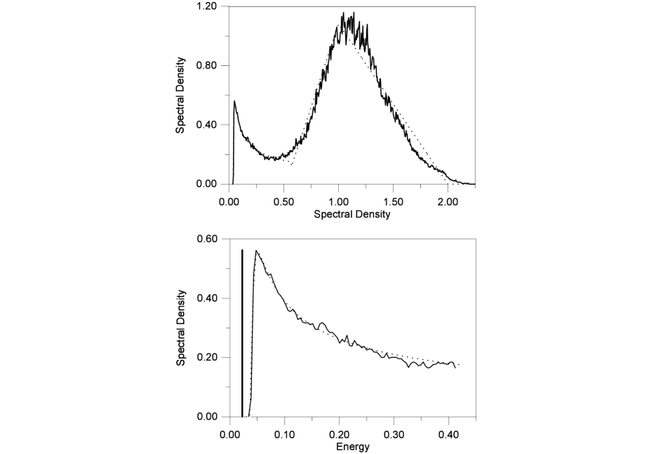
FIG. 16.: Model spectral density (dashed line) and the result of spectral analysis (solid line). The position of the delta-function is shown only in the lower panel.

The Green function $G(\tau)$ was calculated from the model spectral density in the $n_{\mbox{max}}=300$ points $\tau_{i}=\tau_{\mbox{max}}i^{2}/n_{\mbox{max}}$ in the time range from zero to $\tau_{\mbox{max}}=1000$. The restored spectral density reproduces both gross features of high-frequency part (upper panel in Fig. 16) and the fine structure at small frequencies (lower panel of Fig. 16). The energy and the weight of the delta-function was restored with the accuracy $10^{-4}$. The final solution was obtained by the averaging (B4) of $M=1100$ particular solutions.

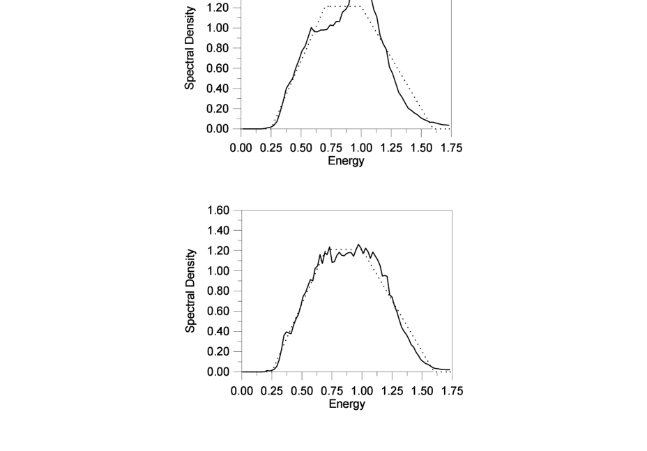
FIG. 17.: The model spectrum (dashed lines) and results of spectral analysis (solid lines) for $\eta=10^{-2}$ (upper panel) and $\eta=10^{-3}$ (lower panel).

To evaluate the precision which characterizes how typical particular solution $\tilde{\rho}_{j}(\omega)$ (see (B3)) reproduces the Green function $G(\tau)$, we introduce the maximal relative deviation

$$\eta=\max\left[\frac{\mid G(\tau_{i})-\tilde{G}(\tau_{i})\mid}{G(\tau_{i})}\right],\;i\in[1,n_{\mbox{max}}]\;,$$ (B29)

which typical value is $\eta=10^{-4}$ for a particular solution of the spectrum in Fig. 16.

Since the Green function which is obtained from Monte Carlo calculations contains some statistic errors at each time point, the minimal value of parameter $\eta$ is limited by the quality of the calculated Green function $G(\tau)$. To study the influence of the (uncorrelated) statistic errors we studied the stability of the method against stochastic noise

$$G(\tau_{i})\to G(\tau_{i})(1+\eta r_{i})\;,\;i=1,n_{\mbox{max}}\;,$$ (B30)

introduced by random numbers $r_{i}\in[0,1]$. It is seen that the method restores the gross features of the spectrum (position and width) even for rather roughly calculated Green function, with $\eta=10^{-2}$ (upper panel in Fig. 17), whereas the precision $\eta=10^{-3}$ is sufficient to resolve the lineshape (lower panel in Fig. 17)).

REFERENCES

- [1] N.V. Prokof’ev and B.V. Svistunov, Phys. Rev. Lett. 81, 2514 (1998).
- [2] J. Appel, in Solid State Physics, edited by H. Ehrenreich, F. Seitz, and D. Turnbull (Academic, New York, 1968), Vol. 21.
- [3] L.D. Landau, Sov. Phys. 3, 664 (1933).
- [4] H. Fröhlich, H. Pelzer, and S. Zienau, Phil. Mag. 41, 221 (1950).
- [5] E.P. Gross, Ann. Phys. 8, 78 (1959).
- [6] D. Matz and B.C. Burkey, Phys. Rev. B 3, 3487 (1971).
- [7] J.M. Luttinger and C.Y. Lu, Phys. Rev. B 21, 4251 (1980).
- [8] R. Mańka, Phys. Lett. A 67, 311 (1978); Phys. Stat. Sol. (b) 93, 53 (1979).
- [9] R. Mańka and M. Suffczynski, J. Phys. C 13, 6369 (1980).
- [10] Y. Lépine and D. Matz, Phys. Stat. Sol. (b) 96, 797 (1979).
- [11] I.D. Feranchuk, S.I. Fisher, and L.I. Komarov, J. Phys. C 18, 5083 (1985).
- [12] F.M. Peeters and J.T. Devreese, Phys. Stat. Sol. (b) 112, 219 (1982).
- [13] R.P. Feynman, Statistical Mechanics, Reading, Benjamin (1972)
- [14] R.P. Feynman, Phys. Rev. 97, 660 (1955).
- [15] T.D. Schultz, Phys. Rev. 116, 526 (1959).
- [16] T.D. Lee, F.E. Low and D. Pines, Phys. Rev. 90, 297 (1953).
- [17] N.V. Prokof’ev, B.V. Svistunov, and I.S. Tupitsyn, Zh. Eksp. Teor. Fiz. 114, 570 (1998) [Sov. Phys. JETP 87, 310 (1998)].
- [18] N. Metropolis et al., J. Chem. Phys., 21, 1087 (1953).
- [19] A.M. Ferrenberg and R.H. Swendsen, Phys. Rev. Lett. 61, 2635 (1988); 63, 1658(E) (1989).
- [20] H. Grabert, Phys. Rev. B 50, 17364 (1994).
- [21] L. D. Landau, S. I. Pekar, Zh. Eksp. Teor. Fiz. 18, 419 (1948).
- [22] D. Pines, in Polarons and Exitons, eds. C.G. Kuper and G.D. Whitfield, Plenum Press, N.Y., 155 (1962).
- [23] L.P. Pitaevskii, Zh. Eksp. Teor. Fiz. 36, 1168 (1959).
- [24] Polarons in Ionic Crystals and Polar Semiconductors, ed. by J. T. Devreese, North-Holland, Amsterdam (1972).
- [25] V. Gurevich, I. Lang and Yu. Firsov, Soviet Phys.- Solid State 4, 918 (1862).
- [26] J. Devreese, W. Huybrechts and L. Lemmens, Phys. Stat. Sol. (b) 48, 77 (1971).
- [27] E. Kartheuser, R. Edvard and J. Devreese, Phys. Rev. Lett. 22, 94 (1969).
- [28] J. Devreese, J. De Sitter and M. Goovaerts, Solid State Comm. 9, 1383 (1971).
- [29] J. Devreese, J. De Sitter and M. Goovaerts, Phys. Rev. B 5, 3367 (1972).
- [30] D.M. Ceperley, J. Comp. Phys. 51, 404 (1983); D.M. Ceperley and B.J. Alder, J. Chem. Phys. 81, 5833 (1984).
- [31] N.V. Prokof’ev, B.V. Svistunov, and I.S. Tupitsyn, Phys. Rev. Lett. 82, 5092 (1999).